

Abstract
Over the last decade there has been a tremendous advance in the analytical tools available to neuroscientists to understand and model neural function. In particular, the point process - Generalized Linear Model (PPGLM) framework has been applied successfully to problems ranging from neuro-endocrine physiology to neural decoding. However, the lack of freely distributed software implementations of published PP-GLM algorithms together with problem-specific modifications required for their use, limit wide application of these techniques. In an effort to make existing PP-GLM methods more accessible to the neuroscience community, we have developed nSTAT – an open source neural spike train analysis toolbox for Matlab®. By adopting an Object-Oriented Programming (OOP) approach, nSTAT allows users to easily manipulate data by performing operations on objects that have an intuitive connection to the experiment (spike trains, covariates, etc.), rather than by dealing with data in vector/matrix form. The algorithms implemented within nSTAT address a number of common problems including computation of peri-stimulus time histograms, quantification of the temporal response properties of neurons, and characterization of neural plasticity within and across trials. nSTAT provides a starting point for exploratory data analysis, allows for simple and systematic building and testing of point process models, and for decoding of stimulus variables based on point process models of neural function. By providing an open-source toolbox, we hope to establish a platform that can be easily used, modified, and extended by the scientific community to address limitations of current techniques and to extend available techniques to more complex problems.
Keywords: Open-Source, Point Process, Generalized Linear Models, Neuroscience, Statistics, Data Analysis, Signal Processing, Spike Trains
1. Introduction
Understanding and quantifying how neurons represent and transmit information is a central problem in neuroscience. Whether it involves understanding how the concentration of a particular chemical present within the bath solution of an isolated neuron affects its spontaneous spiking activity (Phillips et al., 2010) or how a collection of neurons encode arm movement information (Georgopoulos et al., 1986), the neurophysiologist aims to decipher how the individual or collective action potentials of neurons are correlated with the stimulus, condition, or task at hand.
Due to the stereotypic all-or-none nature of action potentials, neural spiking activity can be represented as a point process, a time series that takes on the value 1 at the times of an action potential and is 0 otherwise (Daley and Vere-Jones, 1988). Many other common phenomena can be described as point processes ranging from geyser eruptions (Azzalini and Bowman, 1990) to data traffic within a computer network (Barbarossa et al., 1997). Generalized Linear Models (GLMs) (McCullagh and Nelder, 1989), a flexible generalization of linear regression, can be used in concert with point process models to yield a robust and efficient framework for analyzing neural spike train data. This point process - Generalized Linear Model (PP-GLM) framework has been applied successfully to a broad range of problems including the study of cardiovascular physiology (Chen et al., 2011, 2010a,b, 2008b, 2009a, 2008a, Barbieri and Brown, 2004,Barbieri et al., 2005a, Barbieri and Brown, 2006b,a), neuro-endocrine physiology (Brown et al., 2001), neurophysiology (Schwartz et al., 2006, Frank et al., 2002, 2004, Eden et al., 2004b, Frank et al., 2006, Vidne et al., 2012), and neural decoding (Barbieri et al., 2004, Eden et al., 2004a, Srinivasan et al., 2006, 2007, Barbieri et al., 2008, Wu et al., 2009, Ahmadian et al., 2011). Truccolo et al. (2005) andPaninski et al. (2007) provide a broad overview of the PP-GLM framework.
While much progress has been made on the development and application of PP-GLM methods within neuroscience, the use of these methods typically requires in-depth knowledge of point process theory. Additionally, while there are widely available implementations for the estimation of GLMs within software packages such as Matlab® (The Mathworks, Natick, MA), S, or R programming languages, their use to analyze neural data requires problem specific modifications. These adaptations require much work on the part of the experimentalist and detract from the goal of neural data analysis. These barriers are exacerbated by the fact that even when software implementations are made publicly available they vary greatly in the amount of documentation provided, the programming style used, and in the problem-specific details.
Numerous investigators have successfully addressed common problems within neuroscience (such as spike sorting, data filtering, and spectral analysis) through the creation of freely available software toolboxes. Chronux (Bokil et al., 2010), FIND (previously MEA-Tools) (Meier et al., 2008, Egert et al., 2002), STA-Toolkit (Goldberg et al., 2009), and SPKtool (Liu et al., 2011) are a few examples of such tools. Chronux offers several routines for computing spectra and coherences for both point and continuous processes along with several general purpose routines for extracting specified data segments or binning spike time data. STAToolkit offers robust and well-documented implementations of a range of information-theoretic and entropy-based spike train analysis techniques. The FIND toolbox provides analysis tools to address a range of neural activity data, including discrete series of spike events, continuous time series and imaging data, along with solutions for the simulation of parallel stochastic point processes to model multi-channel spiking activity. SPKtool provides a broad range of tools for spike detection, feature extraction, spike sorting, and spike train analysis. However, a simple software interface to PP-GLM specific techniques is still lacking.
The method for data analysis within the PP-GLM framework is consistent and amenable to implementation as a software toolbox. There are two main types of analysis that can be performed: 1) encoding analysis and 2) decoding analysis. In an encoding analysis, the experimenter seeks to build a model that describes the relationship between spiking activity and a putative stimulus and covariates (Paninski et al., 2007). This type of analysis requires model selection and assessing goodness-of-fit. A decoding analysis estimates the stimulus given spiking activity from one or more neurons (Donoghue, 2002, Rieke, 1999). An example of this type of analysis would aim to estimate arm movement velocity given the population spiking activity of a collection of M1 neurons and a model of their spiking properties such as that developed by Moran and Schwartz (1999).
We use the consistency of the data analysis process within the PP-GLM framework in the design of our neural Spike Train Analysis Toolbox (nSTAT). Our object-oriented software implementation incorporates knowledge of the standard encoding and decoding analysis approaches together with knowledge of the common elements present in most neuroscience experiments (e.g. neural spike trains, covariates, events, and trials) to develop platform that can be used across a broad range of problems with few changes. Object-oriented programming (OOP) represents an attempt to make programs more closely model the way people think about and interact with the world. By adopting an OOP approach for software development we hope to allow the user to easily manipulate data by performing operations on objects that have an intuitive connection to the experiment and hypothesis at hand, rather than by dealing with raw data in matrix/vector form. Building the toolbox for MATLAB®, we make sure that users can easily transfer their data and results from nSTAT to other public or commercial software packages, and develop their own extensions for nSTAT with relative ease.
nSTAT address a number of problems of interest to the neuroscience community including computation of peri-stimulus time histograms, quantification of the temporal response properties of neurons (e.g. refractory period, bursting activity, etc.), characterization of neural plasticity within and across trials, and decoding of stimuli based on models of neural function (which can be pre-specified or estimated using the encoding methods in the toolbox). Importantly, the point process analysis methods within nSTAT are not limited to sorted single-unit spiking activity but can be applied to any binary discrete spiking process such as multi-unit threshold crossing events (see for example Chestek et al. 2011)). It should be noted that while all of the examples presented in the paper focus on the PP-GLM framework, nSTAT contains methods for analyzing spike trains when they are represented by their firing rate and treated as a Gaussian time-series instead of a point process. These include time-series methods such as Kalman Filtering (Kalman, 1960), frequency domain methods like multi-taper spectral estimation (Thomson, 1982), and mixed time-frequency domain methods such as the spectrogram (Cohen and Lee, 1990, Boashash, 1992). For brevity, and because these methods are also available in other toolboxes, we do not discuss these elements of the toolbox herein.
This paper is organized as follows: Section 2.1 summarizes the general theory of point processes and generalized linear models as it applies to our implementation. We include brief descriptions of some of the algorithms present in nSTAT to establish consistent notation across algorithms developed by distinct authors. Section 2.2 describes the software classes that make up nSTAT, the relationships among classes, and relevant class methods and properties. Section 2.3 describes five examples that highlight common problems addressed using the PP-GLM framework and how they can be analyzed using nSTAT. Lastly, results for each of the different examples are summarized in Section 3. nSTAT is available for download at http://www.neurostat.mit.edu/nstat/. All examples described herein (including data, figures, and code) are contained within the toolbox help files. The software documentation also includes descriptions and examples of the time-series methods not discussed herein for brevity.
2. Material and Methods
2.1. Summary of the PP-GLM Framework
In this section, we describe the PP-GLM framework and the model selection and goodness of fit techniques that can be applied within the framework to select among models of varying complexity. The peri-stimulus time histogram (PSTH) and its PP-GLM analogue, the GLM-PSTH, are then presented together with extensions that allow for estimation of both within-trial and across-trial neural dynamics (SSGLM). We then discuss how point process models can be used in decoding applications when neural spiking information is used to estimate a driving stimulus.
2.1.1. Point Process Theory
Due to the stereotyped all-or-none nature of action potentials, neural spiking activity can be represented as a point process, i.e. as a time series that takes on the value 1 at the time of an action potential and is 0 otherwise. Given an observation interval (0, T] and a time t ∈ (0, T], we define the counting process N (t) as the total number of spikes that have occurred in the interval (0, t]. A point process is completely characterized by its conditional intensity function (CIF) (Daley and Vere-Jones, 1988) defined as
| (1) |
where Ht is the history information from 0 up to time t. For any finite Δ, the product λ (t|Ht)Δ is approximately the probability of a single spike in the interval (t, t + Δ] given the history up to time t. The conditional intensity function can be considered a generalization of the rate for a homogeneous Poisson process.
If the observation interval is partitioned into and individual time steps are denoted by Δtj = tj - tj−1, we can refer to each variable by its value within the time step. We denote Nj = N (tj) and refer to ΔNj = Nj -N j−1 as the spike indicator function for the neuron at time tj. If Δtj is sufficiently small, the probability of more than one spike occurring in this interval is negligible, and ΔNj takes on the value 0 if there is no spike in (t j−1, tj] and 1 if there is a spike. In cases where fine temporal resolution of the count process, N (t), is not required we define ΔN (tA, tB) to equal the total number of spikes observed in the interval (tA, tB].
2.1.2. Generalized Linear Models
The exponential family is a broad class of probability models that include many common distributions including the Gaussian, Poisson, binomial, gamma, and inverse Gaussian distributions among many others. The key concept underlying Generalized Linear Models (GLM) (McCullagh and Nelder, 1989) involves expressing the natural parameter of the probability model from the exponential family as a linear function of relevant covariates. Efficient and robust algorithms for linear regression can then be employed for maximum likelihood parameter estimation. Thus if the conditional intensity function is modeled as a member of the exponential family, we have an efficient algorithm for estimating CIF model parameters. Additionally, this approach allows effective selection between competing models via the likelihood criteria described below. In particular, we will use two main types of GLMs for the conditional intensity functions herein:
Poisson regression models where we write log (λ (tj |Htj)Δ) as a linear function of relevant covariates, e.g.
| (2) |
and 2) binomial regression models where we write the inverse of the logistic function, logit (λ (t|Ht)Δ), as a linear function of covariates, e.g.
| (3) |
where is the jth row of the design matrix X and β is the vector of model parameters to be estimated. The spike indicator function, ΔNj, is taken as the observation, termed yj, and is modeled either as a Poisson or binomial random variable. That is .
2.1.3. Model Selection
Goodness of fit measures currently implemented in nSTAT include the time rescaling theorem for point processes (Brown et al., 2002), Akaike’s information criteria (AIC) (Akaike, 1973), and Bayesian information criteria (BIC) (Schwarz, 1978). Briefly, the time rescaling theorem states that given the true conditional intensity function of a point process, λ, and a sequence of spike times 0 < t1 < t2 < … < ts < … < tS < T , the rescaled spike times are defined as
| (4) |
where s = 1, …, S are independent, identically distributed, uniform random variables on the interval (0, 1). To use the time-rescaling theorem to test the model goodness of fit, one can apply Equation 4 to each candidate model, λi, to obtain a set of candidate rescaled spike times that can then be tested for independence and their closeness (to be made precise below) to an uniform distribution.
The Kolmogorov-Smirnov (K-S) test can be used to compare how close the empirical distribution of rescaled spike times, us’s, are to a reference uniform distribution on the interval (0, 1). The visual representation of this test, termed a K-S plot (Brown et al., 2002), together with corresponding confidence intervals (Johnson and Kotz, 1970) allows for comparison of multiple models simultaneously. If the candidate model is correct, the points on the K-S plot should lie on a 45° line (Johnson and Kotz, 1970). The K-S statistic is the largest deviation from the 45° line. Application of the time-rescaling theorem to sampled data produces some artifacts within K-S plots since the actual spike times could have occurred anywhere within the finite-sized time bins. These artifacts are addressed within nSTAT using the discrete time rescaling theorem (Haslinger et al., 2010).
Independence of the rescaled spike times can be assessed by plotting vs. (Truccolo et al., 2005). In this case, a correlation coefficient statistically different from zero casts doubt on the independence of the rescaled spike times. A stronger test for independence uses the fact that uncorrelated Gaussian random variables are also independent. If the are uniform random variables on the interval (0, 1), then
| (5) |
where Φ−1 (·) is the inverse of the standard normal distribution cumulative distribution function (CDF), will be normally distributed with zero mean and unit variance. Significant non-zero coefficients of the auto-correlation function of the at non-zero lags demonstrates that the rescaled spike times are not independent (Truccolo et al., 2005). The 95% confidence interval for the non-zero lag coefficients of the auto-correlation function is ±1.96/ where n is the total number of rescaled spike times.
Goodness of fit can also be assessed by examining the structure of the point process model residuals (Andersen, 1997, Truccolo et al., 2005) defined over non-overlapping moving time windows of size B as
| (6) |
for j - B ≥ 1. Strong correlations between covariates absent from the model for λi and are indicative of potentially important un-modeled effects.
The AIC, BIC, rescaled spike times, and the point process residuals are computed within the nSTAT Analysis class for each candidate model, λi, and stored within the returned FitResult object (see Section 2.2 for more details). The FitResult method plotResults displays the K-S plot, the plot of vs. and corresponding correlation coefficient, the auto-correlation function of the , and the point process residual for each of the candidate λi’s.
2.1.4. Simulating Point Processes
Validation and testing of new algorithms requires generating spiking activity according to known prior behavior. Given an integrable CIF λ (t|Ht) for 0 ≤ t ≤ T, a realization of the point process compatible with this CIF can be generated via time rescaling (Brown et al., 2002) as follows:
Set t0 = 0; Set s = 1.
Draw zs an exponential random variable with mean 1.
Find ts as the solution to .
If ts > T , then stop.
s = s + 1
Go to 2.
In instances where the CIF is independent of history (e.g. a homogenous or inhomogenous Poisson process), the more computationally efficient point process thinning algorithm (Lewis and Shedler, 1978, Ogata, 1981) can be used. The nSTAT CIF class contains static methods (e.g. CIF.simulateCIF, CIF.simulateCIFByThinning, and CIF.simulateCIFByThinningFromLambda) to generate a realization of a point process based on either time rescaling or the point process thinning algorithm.
2.1.5. PSTH and the GLM Framework
In neurophysiology, the peri-stimulus time histogram and post-stimulus time histogram, both abbreviated PSTH or PST histogram, are histograms of the times at which neurons fire. These histograms are used to visualize the rate and timing of neuronal spike discharges in relation to an external stimulus or event. To obtain a PSTH, a spike train recorded from a single neuron is aligned with the onset, or a fixed phase point, of an identical repeatedly presented stimulus. The aligned sequences are superimposed in time and then combined to construct a histogram (Gerstein and Kiang, 1960, Palm et al., 1988).
For concreteness, suppose that a PSTH is to be constructed from spiking activity of a neuron across K trials each of duration T. The time interval T is partitioned into N time bins each of width Δ and the spike trains represented by their value (0 or 1) within each bin. To estimate the firing rate, we partition the time interval T into R time bins (with R > Δ). According to Czanner et al. (2008), the PSTH is a special case of the CIF defined by the following GLM
| (7) |
for k = 1, …, K and n = 1, …, N. Here k and n are the trial number and bin within a trial respectively, and
| (8) |
are the unit pulse functions in the observation interval (0, T] (e.g. g1 (nΔ) = 1 from n = 1, …, NR−1 and zero outside this time interval). This conditional intensity function is the same for all trials k = 1, .., K. Note that since there are R unit pulse functions over the N observed samples, the width of each unit pulse function is NR−1. For the bin in which gr (nΔ) = 1, the spiking activity obeys a homogenous Poisson process with mean rate exp (θr) /Δ, and since the basis functions in Equation 8 are orthogonal, the values exp (θr) /Δ r = 1, …, R can be estimated independently of each other. The maximum-likelihood estimate of exp (θr) /Δ is the number of spikes that occur in the bin in which gr (nΔ) = 1, summed across all trials, and divided by the number of trials and the bin width (e.g. equal to the value of the PSTH in the rth time bin). Within nSTAT, the PSTH and the GLM-PSTH can be computed for any collection of neural spike trains (represented by the class nstColl) by specifying the bin width Δ. The GLM-PSTH routine (psthGLM method) also allows for the estimation of spiking history effect of the same form as described in Section 2.1.6.
2.1.6. State Space GLM Framework
The standard PSTH treats each trial as independent to produce an estimate of the firing rate. In many experiments it is of interest to not only capture the dominant variation in firing rates within a trial, but also to examine changes from one trial to the next (for example to examine neural plasticity or learning). Czanner et al. (2008) formulated the state-space generalized linear model (SSGLM) framework to allow for this type of analysis. Briefly the SSGLM framework proposes that the CIF be modeled as
| (9) |
where k is the current trial index and ΔNk (tA, tB) equals the total number of spikes observed in the interval (tA, tB] of the kth trial. The stochastic trial-to-trial dependence between the parameters θk = [θk,1 … θk,r … θk,R] is described by the random walk model
| (10) |
for k = 1, …, K, where K is the total number of trials, εk is an R-dimensional Gaussian random vector with mean 0 and unknown covariance matrix Σ. The initial vector θ0 is also assumed to be unknown. Because the parameters θk and γj of the GLM and the covariance parameter, Σ, of the random walk model are unknown, an iterative Expectation-Maximization algorithm (Dempster et al., 1977) is employed to estimate them.
The spike rate function on the interval [t1, t2] is defined as
| (11) |
where Λk (t1, t2) corresponds to the expected number of spikes in the interval [t1, t2]. The corresponding maximum likelihood estimate of the spike rate function is obtained by evaluating Equation 11 with the estimated conditional intensity function. Confidence intervals can be constructed via the Monte Carlo methods described byCzanner et al. (2008). Statistical comparisons of the spike rate function between trials can be performed in order to examine experience dependent changes or learning across trials. In particular, for a given interval [t1, t2] and trials m and k we can compute the maximum-likelihood estimates of Equation 11 and use Monte Carlo methods to compute
| (12) |
for any k = 1, …, K - 1 and m > k. The smallest m such that probability in Equation 12 is greater than or equal to 95% is denoted as the learning trial with respect to trial k (i.e. the first trial where the spike rate function in the time interval [t1, t2] is significantly different than the spike rate function in trial k).
The SSGLM algorithm is implemented by the nstColl class and requires specification of the number of J + 1 time points ([t0, t1, …, tJ]) that are used to construct J time windows of prior spiking activity, along with the number of within-trial bins, R, to be used. The method returns estimates of θk for k = 1, …, K; Σ; and γ = [γ1, …, γJ].
2.1.7. Point Process Adaptive Filter
In some situations, one has prior knowledge of the form of the conditional intensity function, λc (t|x (t), θ, Ht) for c = 1, …, C, where C is the number of individual neurons being observed, x(t) is a vector of stimuli/covariates of interest, θ is a vector of parameters (typically obtained via GLM), and Ht is all of the relevant history up to time t. The decoding problem is then, given a collection of CIFs, to estimate the stimuli/covariates x(t) = [x1 (t) … xN (t)]T based on the spiking activity of the ensemble ΔN1:C (t). It is customary to discretize time and adopt the notation xk = x (t) | t=kT. We denote the spiking activity in the kth time step by the vector of binned spike counts. The cth element of contains the total number of of spikes generated by the cth neuron in the kth time step. Spike history is represented by .
The system of equations for the state (stimuli) vector are defined as
where Ak is the state transition matrix and ωk is a zero mean Gaussian random vector with covariance Qk. The effect of the stimuli is only observed via the spiking of each of the individual cells, i.e.,
| (13) |
for c = 1, …, C, where p denotes the conditional probability distribution function of a spike in the kth time bin by the cth cell conditioned on the current stimulus, xk, and history. Decoding is then equivalent to estimating the posterior density, . From Bayes rule,
| (14) |
The second term in the numerator of Equation 14 is the one-step prediction density defined by the Chapman-Kolmogorov equation as
| (15) |
Eden et al. (2004a) proposed a Gaussian approximation to this posterior and demonstrated that the recursive estimates for the stimulus mean and covariance at time k are given by the point process adaptive filter (PPAF) equations.
Prediction:
| (16) |
| (17) |
Update:
| (18) |
| (19) |
If the final state xK is known (e.g. reaching to a known target), the point process adaptive filter can be modified according toSrinivasan et al. (2006) so that the final state estimate matches the known final state. Decoding of both discrete and continuous states, sk and xk respectively, from point process observations termed the Point Process Hybrid Filter (PPHF) was derived by Srinivasan et al. (2007). The equations for the PPHF are not reproduced here for brevity but are implemented within nSTAT.
The PPAF is implemented by the PPDecodeFilter and PPDecodeFilterLinear methods of the DecodingAlgorithms class. It requires the specification of the state transition matrix, Ak, the covariance matrix, Qk, a description of the CIF for each cell, the observed spiking activity, for k = 1, …, K, and optionally target specific information. The method returns estimates of states xk|k and xk+1|k, and the corresponding covariances Wk|k and Wk+1|k. The PPHF is implemented by the PPHybridFilter and PPHybridFilterLinear methods of the DecodingAlgorithms class. It requires the specification of the matrices, and for each possible value of the the discrete state, sk, a description of the CIF for each cell under for each value of sk, the observed spiking activity, for k = 1, …, K, a matrix of state transition probabilities p(sk|sk−1), and optionally target-specific information. The method returns estimates of sk|k, xk|k and Wk|k.
2.2. Object Oriented Program Structure
Object oriented programming (OOP) is a programming language model that is organized around “objects” – data structures consisting of data fields and methods. Objects are specified by their class definitions which specify the fundamental properties of the object and how the data within the object can be manipulated. This programming approach allows for inheritance - the notion that a more sophisticated class can reuse the properties and methods of elementary classes. The PP-GLM framework consists of some fundamental elements that lend themselves directly into this model. While the specific applications and experiments might range widely, encoding and decoding analysis within the framework often consists of the same basic elements: spike trains, covariates, trials, and events within trials. The benefits of this approach are
Data Encapsulation: Once an object is created, it can be manipulated only in the ways pre-specified by the class. The helps maintain the consistency of the data as the object is manipulated during the analysis process. This encapsulation is essential for complex problems where specific implementation details might become overwhelming. For example, when manipulating an object of the Trial class, users need not focus on the implementation details of spike trains (class nspikeTrain), covariates (class Covariate), and events (class Event), but can rather perform operations on trials as a whole via the methods provided by the Trial class.
Method access: Each class has methods that are relevant to it and the type of information that it contains. This helps users know what kinds of operations can be performed on different types of objects.
-
Code reuse: Due to inheritance, methods need not be implemented for each new object. This leads to organization of methods across classes and simplified code maintenance. This property also improves code testing and maintenance by yielding increased code clarity and readability. For example, consider the computation of the time rescaling theorem. Suppose we have a collection of spike times, 0 < t1 < t2 < … < ts < … < tS < T, represented as a vector called spikeTimes, and a conditional intensity function, λ (t|Ht), represented as a SignalObj called lambda. The rescaled spike times, us, from the time rescaling theorem are computed by the following code:
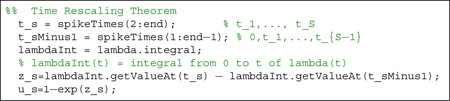
where the integral method of class SignalObj returns a SignalObj object. Since lambdaInt is an object of class SignalObj it has a getValueAt method that can be used to obtain the value of the integral at each of the spike times in the vectors t_s and t_sMinus1.

Figure 1 highlights how the standard PP-GLM workflow is related to the nSTAT classes, and how a particular problem can be analyzed using nSTAT. In this case, the included code corresponds to the first portion of Example 1. Figure 2 uses unified modeling language (UML) formalism (Booch et al., 2005, Bézivin and Muller, 1999) to show how the classes that make up nSTAT are related.
Figure 1. Visual overview of the data analysis workflow, relevant classes, and code using nSTAT.

This particular example shows the typical workflow in the testing of candidate conditional intensity functions. For brevity, the workflow for decoding stimuli using the Point Process Adaptive Filter or the Hybrid Point Process Filter is not shown (see the Matlab help files for these examples for the corresponding code).
Figure 2. Class Diagrams.

A) Unified Modeling Language (UML) representation of the classes that implement the encoding and decoding analysis methods and store the relevant results. B) UML diagram of the remaining classes within nSTAT.
2.2.1. nSTAT Classes
SignalObj - a class representing a signal abstraction. In general, a signal is any time-varying or spatially-varying quantity (e.g. a time-series). This implementation of the signal abstraction consists of the pair (t, x (t)), where t is a one-dimensional indexing variable (time, space, etc.) and x (t) is the corresponding data specified at each value of the indexing variable. A signal can be multivariate if at every value of the indexing variable, a vector of data is specified (the size of this vector determines the dimension of the signal). SignalObj’s have a number of methods that facilitate the manipulation of their data such as maxima, minima, frequency spectra, etc. SignalObj’s can be integrated, differentiated, filtered, shifted, scaled, added, and subtracted among other operations and the result of these operations is also a SignalObj.
Covariate - a class representing the explanatory variables used in the construction of conditional intensity function models within the PP-GLM framework. Covariates are SignalObj’s with mean μ and standard deviation σ.
CovColl - a container for multiple Covariate objects. This container ensures that all the covariates have the same sampling rate, start time, and end time. CovColl has a covMask field that allows some Covariates to be masked or effectively hidden from the current analysis. Additionally, the CovColl can be converted to a matrix by the dataToMatrix method. Only covariates that are currently selected in the covMask field are used in the creation of the matrix representation of the CovColl. This matrix representation is used to generate part of the design matrix, X, for GLM analysis (see Equations 2 and 3). The other portions of the design matrix are determined by the number history windows specified by the History object in the current TrialConfig.
nspikeTrain - a neural spike train object consists of a set of spike times. The spike train can be represented as a signal of class SignalObj with a particular sampling rate. Note that if the bin size resulting from the specified sample rate is larger than the difference between any two spike times, the neural spike train will not have a binary SignalObj representation. Effectively, specification of sample rate for an object of class nspikeTrain specifies how the spike train will be binned.
nstColl - a container for objects of class nspikeTrain that ensures that all the contained spike trains have the same start time, end time, and sample rate. Similar to covColl, nstColl has a neuronMask field that allows selection of a subset of all the spike trains in the collection. nstColl includes methods for the generation of inter-spike interval (ISI) histograms and peri-stimulus time histograms (PSTH). The method dataToMatrix can be used to obtain a matrix representation of the spike trains that is used by the Analysis class to obtain the observations, yj = ΔN (tj), used in GLM analysis.
Event - consists of a collection of pairs of times and labels, (tk, ℓk), that are used to identify important time-points within Trial objects.
History - defines a collection of time window edges/boundaries within which the spiking activity of a nspikeTrain is to be analyzed. For example the vector of window times, [0, 0.002, 0.01], specifies one window from 0 to 2 ms and another from 2 ms to 10 ms. Calling the computeHistory method on a spike train using the previously mentioned window times would yield a Covariate object with two dimensions. The first dimension would be a time-series that at time t has the value of the summed spiking activity in the interval [t - 2, t) (e.g. the summed spiking activity of the prior 2 ms) and the second a time-series that at time t equals the sum of the spiking activity in the interval [t - 10, t - 2) (e.g. the summed spiking activity from 2 ms to 10 ms in the past).
Trial - consists of covColl, nstColl, and Event objects and implements the abstraction of an experimental trial by keeping all of the corresponding data together. The trial data can be visualized using the plot method. This class ensures that the spike trains and covariates are all properly sampled and aligned in time.
TrialConfig - a class that specifies the manner in which a Trial object should be analyzed. Each TrialConfig object specifies the name of the covariates to be included in the analysis, the sample rate to be used for all of the covariates and spike trains, the history windows to be used, and the time window for analysis (i.e. can perform analysis on a subset of all the trial data).
ConfColl - a container for multiple TrialConfig objects.
Analysis - a collection of static methods for analyzing a Trial according to the specifications included in a ConfigColl. Given a Trial and ConfigColl object, the method RunAnalysisForAllNeurons returns a FitResult object for each spike train in the trial. Each FitResult object contains the results of all the different configurations specified in the ConfigColl as applied to each spike train.
FitResult - contains the GLM coefficients (with corresponding standard errors), AIC, BIC, KS statistics, rescaled spike times, and point process residual for each of the specified configurations in ConfigColl. Includes methods to visualize the results of each of the different configurations to assist in the model selection process. For example, the plotResults method overlays the KS plot, the autocorrelation function of the , the lag−1 correlation coefficient of the , the GLM fit coefficients with 95% confidence intervals, and the point process residual for each of the models specified in the ConfigColl.
FitResSummary - given a collection of FitResult objects (one for each neuron, each containing the results of multiple regressions), computes summary statistics across all neurons and all configurations in the ConfigColl. This class allows visualization of commonalities in the data across multiple neurons.
CIF - conditional Intensity Function abstraction. Allows a conditional intensity function to be defined symbolically. Symbolic differentiation of the CIF can be performed to compute the Jacobian and Hessian of log (λc (t|x(t), θ, Ht)Δ) and λc (t|x(t), θ, Ht)Δ required for computation within the point process adaptive filter or the point process hybrid filter. The CIF class also contains static functions that allow simulating point processes based on specification of the conditional intensity function via time rescaling or the point process thinning algorithm.
DecodingAlgorithms - includes static methods that implement the point process adaptive filter (PPAF), the state-space GLM (SSGLM) filter, and the point process hybrid filter (PPHF) among others. This class also implements non-point process algorithms such as the Kalman Filter (Kalman, 1960) and the Kalman Smoother (Rauch et al., 1965).
2.3. Examples
2.3.1. Example 1 - Homogeneous/Inhomogenous Poisson Models - The Miniature Excitatory Post-Synaptic Current
Miniature excitatory post-synaptic currents (mEPSCs) have become a primary measure of synaptic modification during development, plasticity, and disease. These post-synaptic currents (or “mini’s” ) represent the response of postsynaptic receptors to the spontaneous fusion of vesicles in the pre-synaptic membranes. Recent work byPhillips et al. (2010) has shown that the arrival of mEPSCs under a constant concentration of magnesium is well described as a homogenous Poisson process (i.e. the time between mEPSCs is exponentially distributed). Additionally, as the magnesium concentration is decreased, the rate of mEPSC arrivals begins to increase.
We illustrate the use of nSTAT to analyze the arrival of mEPSCs under two distinct experimental conditions. First, we confirm homogeneous Poisson behavior under constant magnesium conditions by fitting a constant conditional intensity function model to the data in Figure 3, e.g.
| (20) |
and refer to this CIF as λCONST.
Figure 3. Example 1 Data.

A) Experimental Setup B) mini Excitatory Post-Synaptic Currents under a constant Magnesium concentration. C) mEPSCs as the magnesium concentration of the bath is reduced. (Image in panel A courtesy of Marnie Phillips, PhD)
As seen in Figure 3C, when the magnesium concentration in decreased, the rate of mEPSC arrivals increases over time. There are many potential ways to analyze how the underlying firing rate changes with time. For example, under the assumption that the form of the conditional intensity function remains the same as Equation 20 we could decode the rate parameter, μ (t), using the Point Process Adaptive Filter described in Section 2.1.7 and used in Example 2.3.5. However, in this example we take a simpler approach. The spike train is visually separated into three distinct epochs where the baseline firing rates are assumed to be constant within each epoch (shown in Figure 3). Under this assumption, we fit a piecewise constant conditional intensity function
| (21) |
We refer to this CIF as λCONST-EPOCH since it is constant within each time epoch. For comparison, we also fit the constant baseline model of Equation 20 to this data.
2.3.2. Example 2 - Neural Responses in the presence of a known external stimulus (Whisker Stimulus/Thalamic Neurons)
In many experimental settings, the stimulus is directly controlled. In these cases it is of interest to understand how the stimulus modulates the neural spiking. To illustrate we use a sample data set that has been summarized previously by Temereanca and Simons (2003), Temereanca et al. (2008). Briefly, a piezoelectric stimulator was used to caudally deflect the principal whisker (e.g. the whisker that evoked the most robust response from an isolated thalamocortical unit in the ventral posteromedial nucleus). In the data shown here, the whisker was deflected 1mm in the caudal direction beginning from the whisker’s neutral position at a velocity of 80 mm/s for 2 sec with inter-stimulus interval of 1.5 sec.
Given such a data set, several important neurophysiologic questions become of interest: 1) Is there a significant modulatory effect of the stimulus on the neural spiking? 2) What is the temporal relationship (lead vs. lag) of the neural response to the applied stimulus? 3) Does the neural spiking behave as a simple inhomogenous Poisson process or is there a significant history effect (refractoriness, etc.)? 4) If there is a significant history effect, over what time period is this effect important?
In order to address these questions, we proceed as follows
We fit a constant baseline conditional intensity function, λCONST, as in Equation 20.
We look at the cross-correlation between the point process residual MCONST (tk) (see Equation 6) for the λCONST fit and the known stimulus, s(t), to determine the stimulus lag, τlag.
- We fit a baseline plus stimulus model
and refer to this CIF as λCONST+STIM.(22) - We use model selection techniques to determine the number of history windows to include in a model with 30 logarithmically spaced history windows in the past 1 sec. That is
where ΔN (t - tj−1, t - tj) is the total number of spikes that occurred in the time interval [t - tj−1, t - tj) and J is the number of history windows to be determined via model selection. The time windows are defined such that t1 = 0, t30 = 1, and tj for 2 < j < 29 are logarithmically spaced between 0 and 1. We refer to this CIF as λCONST+STIM+HIST.(23) Having determined the “optimal” number of history windows (via AIC, BIC, and K-S statistics), we compare the three candidate conditional intensity functions λCONST, λCONST+STIM, and λCONST+HIST+STIM using the time-rescaling theorem (KS statistic and rescaled spike times), GLM regression coefficients and their significance, and the point process residuals for each model.
2.3.3. Example 3 - Neural Responses to an unknown/implicit stimulus
Recording single-neuron activity from a specific brain region across multiple trials in response to the same stimulus or execution of the same behavioral task is a common neurophysiology protocol. In order to capture the effective neural stimulus that results from the applied physical stimulus, many investigators turn to the peri-stimulus time histogram. To illustrate the construction of PSTH based on a neural raster using nSTAT, we use both simulated and actual data. In Figure 5 A, the point process thinning algorithm was used to generate 20 realizations of a point process governed by the conditional intensity function
| (24) |
where f = 2 and μ = −3.
Figure 5. Example 3 PSTH Data.

Simulated and Actual Data for PSTH Computation. A) (top) graph of λ (t) from Equation 24 (bottom) 20 simulated point process sample paths obtained from the conditional intensity function in Equation 24 via the Point Process Thinning Algorithm. B) 9 trials of stimulus exposure to a V1 neuron for 2 seconds. C) Same as B) with different neuron. Note that the timescale (x-axis range) across the plots is not identical.
Figure 5 B and C show the response of two V1 neurons when a visual stimulus was shown to an adult monkey during a fixation period in response to a moving bar. This data has been published previously (Pipa et al., 2012).
SGLM-PSTH. To demonstrate how the SSGLMframework described in Section 2.1.6 can be applied to estimate both within-trial and across-trial effects we simulate the following conditional intensity function
| (25) |
| (26) |
where λ (k, tn|Htn) is the CIF in the nth time bin of the kth trial, μ = −3 (corresponds to a baseline firing rate of approximately 50 Hertz), Δ = .001 s, f = 2, K = 50 is the total number of trials, J = 3, tj = j milliseconds for j = 0, …, J, and γ = [γ1 γ2 γ3]T =[−4 −1 −0.5]T. The inclusion of the history term models the refractory period of the cell. We refer to sin (2πft) as the within-trial stimulus (since it is consistent across all trials) and bk as the acrosstrial stimulus. The aim of the SSGLM framework is to estimate the history parameter vector, γ, and the non-history dependent stimulus parameters. The SSGLM framework returns an estimate of the stimulus-dependent component of the CIF, e.g.
| (27) |
for k = 1, …, 50.
2.3.4. Example 4 - Neural Responses to a continuous stimulus - Hippocampal place cells
In the rat hippocampus (a region of the brain important for long-term memory formation) pyramidal neurons known as place cells form spatial receptive fields as the animal forages in its environment (O’Keefe and Dostrovsky, 1971, O’Keefe, 1976, O’Keefe and Conway, 1978). In order to show how the spatial receptive fields can be estimated using nSTAT, we reconsider the analysis of Barbieri et al. (2005b) which compared the accuracy of receptive fields constructed using a Gaussian kernel versus Zernike polynomials. Briefly, a Long-Evans rat was allowed to freely forage in a circular environment 70 cm in diameter with 30 cm high walls and a fixed visual cue. A multi-electrode array was implanted into the CA1 region of the hippocampus. The simultaneous activity of 49 place cells was recorded from the electrode array while the animal foraged in the open circular environment for 25 min. Simultaneous with the recording of the place cell activity, the position was measured at 30 Hz by a camera tracking the location of two infrared diodes mounted on the animal’s head stage. Figure 7 shows the response of 4 randomly selected cells.
Figure 7. Example 4 Data.

Hippocampal neural spiking during free foraging. Four cells recorded while a rat was freely foraging in a circular environment. The x-y position at which the cell fires is denoted in red and superimposed on the path of the freely foraging rat in blue. Note that each cell tends to fire near certain locations more than others. The goal in experiments such as this one is to estimate the receptive field or “place” field of each cell based on the recorded spiking activity.
Estimation of the spatial receptive fields using a Gaussian kernel is equivalent to finding the mean, covariance, and baseline firing rate for the conditional intensity function, λG, defined as
| (28) |
where α is the baseline firing rate, x (t) = [x (t), y (t)]T is the normalized position vector of the rat consisting of the x and y coordinates of the rat within the circular environment, and μ the mean and Q the covariance of the two-dimensional Gaussian kernel respectively. Here θG represents the parameters on the right hand side of Equation 28. In order to perform the model fits we need to specify the covariates that will be used in the GLM regression. We expand Equation 28 and rewrite in standard matrix notation as
| (29) |
where 1 is a vector with every element equal to 1 and of appropriate length, XG (t) = [1 x (t) x (t)2 y (t) y (t)2 x (t) · y (t)] is a row vector of the terms from Equation 28 in each column, and βG a column vector of parameters to be estimated. The design matrix, XG, is obtained by placing the data for each time point, t, in subsequent rows. We define each of the columns of the design matrix, XG, as a Covariate object for the fitting of the GLM in Equation 29. The second model for the conditional intensity function, corresponding to the Zernike polynomial basis, λZ, is defined as
| (30) |
where is the mth component of the lth order Zernike polynomial, p (t) = [ρ (t), ϕ (t)] is the polar coordinate representation of the Cartesian position vector x (t) and . We rewrite the equation in matrix notation
| (31) |
| (32) |
where the notation has been replaced by an ordered numbering of the 10 unique non-zero Zernike polynomials for L = 3 as used byBarbieri et al. (2005b). We define each of the columns of the design matrix, XZ, as a Covariate for the fitting of the GLM in Equation 31.
2.3.5. Example 5 - Decoding Continuous Stimuli based on Point Process Models
Decoding a driving stimulus from Point Process Observations
Suppose we have a collection of c = 1, …, C cells with conditional intensity function
| (33) |
as shown in Figure 8. We define the stimulus x (t) = sin (2πft) and aim to obtain an estimate x̂ (t) of the true stimulus x (t) based on the ensemble spiking activity ΔN1:C (t) and knowledge of each λc (t). For this example we choose, C = 20, f = 2, b0 ~ 𝒩 (μ = −4.6, σ = 1), and b1 ~ 𝒩 (μ = 0, σ = 1). A value of b0 = −4.6 corresponds to a baseline firing rate of approximately 10 spikes/sec. Simulated spike trains for each cell, obtained via the point process thinning algorithm, are shown in Figure 8.
Figure 8. Example 5 Driving Stimulus Data.

(top) Driving stimulus, (middle) conditional intensity function for each cell, (bottom) raster of simulated cells begin driven by a sinusoidal stimulus.
Decoding a movement trajectory from Point Process Observations
Suppose that we have a collection of cells c = 1, …, C with condition intensity function adapted from a model of primary motor cortex (Moran and Schwartz, 1999, Srinivasan et al., 2006)
| (34) |
where υx and υy are velocities of the arm end-effector in orthogonal directions. An arm reach from an initial position, x0 = [0, 0]T , to a target at x0 = [−35, 20]T cm was simulated using the reach-to-target equation in (Srinivasan et al., 2006). The resulting velocities were used to generated a CIF according to Equation 34 and neural rasters were generated using the point process thinning algorithm. The final and initial state covariances were Λx0 = ΛxT = ε × I4×4, where ε = 10−6 and I4×4 is the 4 × 4 identity matrix. The corresponding receptive field parameters were selected so that each cell had preferred direction uniformly distributed between −π and π, and ~ 𝒩 (μ = −4.6, σ = 1). The same velocity information was used to simulate the spiking of C = 20 distinct cells 20 times to show how the algorithm performed in the presence of varying cell responses.
3. Results
3.1. Example 1 - Constant and piece wise constant Poisson process - The Miniature Excitatory Post-Synaptic Current
Figure 10 summarizes the results of mEPSC data in Example 1. Under constant magnesium concentrations, the mEPSC data is well fit by the constant conditional intensity function in Equation 20, suggesting that the inter-spike-interval (ISI) distribution for the mEPSC events is well described by an exponential distribution. The KS plot for λCONST lies within the 95% confidence bounds. The autocorrelation function of the xs’s help us determine that the transformed times are also independent. Together, these results indicate that λCONST is a good approximation to the true underlying CIF describing the mEPSC process under constant magnesium concentrations.
Figure 10. Example 1 Results.

A) nSTAT results summary for the constant baseline firing rate model (Equation 20) for the mEPSC data in Figure 3 B). (top, left to right) original neural raster, autocorrelation function of the us’s, K-S Plot, and conditional intensity function estimate. B) (top, left to right) Raster of mEPSC data under varying magnesium concentration, autocorrelation function of the us’s, K-S Plot and CIF estimate. Note that the piecewise constant rate model yields a K-S plot that falls within the 95% confidence bands and produces rescaled event times whose autocorrelation function is closer to zero across all lags – suggesting independence of the rescaled times under λCONST-EPOCH. The estimated CIF (lower right panel) is able to capture the increased rate that is observed in Figure 3 C).
Figure 10 B shows a comparison of the constant rate model in Equation 20 and the piecewise constant rate model in Equation 21. Since both the K-S plot and the autocorrelation function of the xs’s for the piecewise constant model lie within the 95% confidence interval, we conclude λCONST-EPOCH more adequately approximates the true underlying CIF describing the mEPSC activity under varying magnesium concentrations.
3.2. Example 2 - Neural Responses in the presence of a known external stimulus Whisker Stimulus/Thalamic Neurons
Figure 11 summarizes the results of the analysis presented in Section 2.3.2. Analysis of the cross-correlation function between the point process residual from the model in Equation 20 and the whisker-deflection stimulus demonstrates that the neural spiking lags the stimulus by 119 ms. Changes in AIC, BIC and KS statistic are shown in Figure 11 B for increasing values of J and indicate that J = 9 history windows is most consistent with the data (red star). Figure 11 D demonstrates how this length of history captures important temporal properties of the neuron including the refractory period and bursting (i.e. increased spiking probability when last spike occurred in the last 1–5ms). Additionally, the GLM regression coefficient for the baseline firing rate indicates that the neuron has a baseline rate of exp (−5) /Δ ≈ 6.5 Hz and that the increased whisker displacement (positive stimulus) has an excitatory effect on the neural spiking. Lastly, Figure 11 demonstrates that λCONST+STIM+HIST yields a K-S plot that lies within the 95% confidence interval and thus is an adequate description of the true underlying CIF according to the time rescaling theorem.
Figure 11. Example 2 Results.

A) Cross-correlation of the constant baseline model residual, MCONST (t), with the stimulus, s (t). The peak at 0.119 seconds (solid red circle) suggests that the neural activity lags the stimulus by just over 100ms. B) Model selection for number of history windows. The model in Equation 21 was fit for J = 1, …, 30. A minimum in the AIC, BIC, and KS-statistic (denoted by the red *) is observed when J = 9 (9 logarithmically spaced time windows over the interval [0, 12ms]), suggesting this as the best choice for the length of history dependence. C) K-S Plot comparison of λCONST, λCONST+STIM, and λCONST+STIM+HIST . Inclusion of the stimulus effect yields an improvement in the K-S plot but the resulting model does not fall within the 95% confidence bands. Addition of the history dependence produces a K-S plot that does fall within the 95% confidence bands. D) GLM coefficients for all three candidate models (* indicate statistically significant coefficients, p<0.05). Note that the history coefficients capture an initial refractory period (within the first 1ms of spiking), a region of increased spiking probability shortly thereafter (from 1ms–5ms) corresponding to the bursting seen in the absence of the stimulus, and a subsequent period of decreased spiking probability.
3.3. Example 3 - Neural Responses in the presence of an unknown/implicit stimulus
3.3.1. PSTH
Figure 12 compares estimation of PSTH via the standard approach (Gerstein and Kiang, 1960, Palm et al., 1988) and using the GLM formulation of Czanner et al. (2008). Note that the standard PSTH and the PSTH-GLM match exactly.
Figure 12. Example 3 PSTH Results.

A) (top) Raster of 20 cells obtained from the conditional intensity function in Equation 24 via the point process thinning algorithm. (bottom) Comparison of PSTH (red) and PSTH-GLM (black) with 50ms seconds bins to the actual conditional intensity function (blue). Note that the standard PSTH and the PSTH-GLM match exactly. Confidence bands for the PSTH-GLM are shown by the opaque black lines. B) Neuron #6 raster (top) with corresponding PSTH and PSTH-GLM (bottom). C) Neuron #1 raster (top) and corresponding PSTH and PSTH-GLM (bottom). Confidence bands for the PSTH-GLM are indicated by the thin black lines.
3.3.2. SSGLM-PSTH
Figure 13 summarizes the application of the standard PSTH and SSGLM frameworks to the data in Figure 6. As shown in Figure 13 A and B, the SSGLM estimate of the stimulus effect with 40ms bins is in close agreement with the true underlying stimulus effect. The standard PSTH method (also using 40ms bins) fails to capture the across-trial dynamics (because of its assumption that all of the trials are identical and independent) but is able to capture the within-trial dynamics grossly.
Figure 13. Example 3 SSGLM Results.

A) SSGLM Estimated versus actual stimulus response. Both the PSTH and SSGLM estimates partitioned the time axis using 40 ms time bins. B) Comparison of PSTH, SSGLM, and actual stimulus response. C) Plot of the spike rate function, (t2 - t1)−1 Λk (t1, t2), for k = 1, …, 50 and the learning trial estimate obtained by computation of the probability in Equation 12 (shown in 13 E for all trials). The learning trial, trial 9, is indicated by the vertical red line. D) Comparison of the within-trial spike firing rate (stimulus effect) between the baseline (first) trial and the learning trial for comparison. E) Spike rate function comparison matrix. The probability in Equation 12 was computed for k = 1, …, 49 and m > k. For each trial k on the vertical axis, the * indicates which trials m > k (on the horizontal axis) have an estimated spike rate function that is greater than the spike rate function at trial k with probability greater than 95%.
Figure 6. Example 3 SSGLM Data.

Time varying stimulus response. The within-trial stimulus is modulated by the across-trial stimulus gain in order to simulate neural plasticity across trials. . The simulated neural raster is generated via the time rescaling algorithm described in Section2.1.4 using the nSTAT CIF class. The true conditional intensity function is obtained from Equation 27.
3.4. Example 4 - Neural Responses in the presence of a continuous stimulus - Hippocampal place cells
As demonstrated byBarbieri et al. (2005b), the Zernike polynomial model gave a more accurate and parsimonious description of the individual place fields according to both Akaike and Bayesian Information Criterion (see Figure 14 D). The Zernike place field estimates were concentrated in a smaller area and had a wider range of asymmetric shapes (Figure 14 A versus Figure 14 B).
Figure 14. Example 4 Results.

Hippocampal place cell receptive field estimates. A) Gaussian Place fields. B) Zernike place fields. Note that the place fields estimated with the Zernike polynomial basis are able to capture receptive field asymmetries better than the Gaussian estimates. C) Comparison of Zernike and Gaussian receptive field for cell #25. The Gaussian fit is in blue and the Zernike polynomial fit is in green. D) Box plot of change in KS statistics, AIC and BIC across all 49 cells computed as value of statistic in the Gaussian fit minus the value in the Zernike polynomial fit. Note that while the median KS statistics using Gaussian or Zernike basis are similar, the model corresponding to the Zernike receptive fields yield an improvement in terms of the change in AIC and BIC - indicating that the Zernike polynomial models are better fits to the data. Note that for some cells (the outliers marked in red), the improvement is quite dramatic with the use of the Zernike polynomials.
3.5. Example 5 - Decoding Continuous Stimuli based on Point Process Models
3.5.1. Decoding a driving stimulus from Point Process Observations
Figure 15 shows the results of decoding the sinusoidal stimulus in Equation 33 using 20 cells. Note that even though the original neural raster in Figure 8 showed very little correspondence to the driving stimulus, the aggregate information across the population of cells was sufficient to yield an adequate estimate of the stimulus.
Figure 15. Example 5 Results.

A) Stimulus decoding using the point process adaptive filter. The spiking activity of the 20 simulated cells was used with the PPAF in order to decode the stimulus in Equation 24. The estimated stimulus is shown in black with the corresponding 95% confidence intervals illustrated by surrounding lines in black. The actual stimulus is shown in blue. B) Decoded movement trajectory using the PPAF (green) and the PPAF with target information (blue). For each trace, the true velocity information was used to simulate the spiking of 20 distinct cells according to Equation 34 using the point process thinning algorithm. Each cell had a randomly chosen preferred direction. This process was repeated 20 times to show how the algorithms performed in the presence of different cell populations. (top) The PPAF+Goal estimated path in a more faithful reconstruction of the true movement path and shows significantly less variability in across the 20 simulations. Note, however, that comparison the actual movement trajectories shows that the PPAF without goal information is more closely able to track the actual movement dynamics (albeit with significant variability). As the covariance of the final target increases (i.e. certainty in the final target decreases), the PPAF+Goal estimated trajectories become more similar to the PPAF estimates (data not shown).
3.5.2. Decoding a movement trajectory from Point Process Observations
Figure 15 B shows the results of decoding a simulated reach using the point process adaptive filter (green) and the point process adaptive filter with the addition of target information (blue). Note that inclusion of target information causes deviation from the actual movement trajectories, but results in improved estimates of the true movement path and ensures arrival at the final target. When the target information is not present, the PPAF tracks the true trajectories more reliably (albeit with larger variability) but rarely reaches the true final target. As the degree of certainty in the final target is decreased (i.e. the final target covariance increases), the decoded trajectories become increasingly similar to the standard PPAF without target information.
4. Discussion
We have developed the neural Spike Train Analysis Toolbox (nSTAT) for Matlab® to facilitate the use of the Point Process - Generalized Linear Model framework by the neuroscience community. By providing a simple software interface to PP-GLM specific techniques within the Matlab® environment, users of a number of existing open source toolboxes (i.e. Chronux, STAToolkit, etc.) will be able to easily integrate these techniques into their workflow. It is our hope that making nSTAT available in an open-source manner will shorten the gap between innovation in the development of new data analytic techniques and their practical application within the scientific community. For the neurophysiologist, we hope the availability of such a tool will allow them to quickly test the range of available methods with their data and use the results to both inform the quality of their data and refine the protocols of their experiments.
Via a series of examples we have demonstrated the use of the toolbox to solve many common neuroscience problems including: 1) systematic building of models of neural spiking, 2) characterization of explicit experimental stimulus effects on neural spiking, 3) spike rate estimation using the PSTH and extensions of the PSTH (SSGLM) that allow quantification of experience-dependent plasticity (across-trial effects), 4) receptive field estimation, and 5) decoding stimuli such as movement trajectories based on models of neural firing. All of the data, code, and figures used here are included as part of the toolbox. We hope that users will be able to easily modify these examples and use them as a starting point for analysis of their own data.
While the current release of nSTAT contains many commonly used algorithms for analysis of neural data within the PP-GLM framework, there are many avenues for future improvement. In particular, optimization of current algorithm implementations to support the GPU- and parallel-computing methods within Matlab® are likely to be important for dealing with large data sets. We encourage users to identify areas were the software can be made more efficient and to make their contributions available to the community at large. Future work for nSTAT will include the addition of methods to deal with simultaneous analysis of neural ensembles using multivariate point-process theory together with multinomial generalized linear models (mGLMs) (Chen et al., 2009b, Ba, 2011, Brown et al., 2004), network analysis of multivariate spike trains(Brown et al., 2004, Krumin and Shoham, 2010, Stam and Reijneveld, 2007, Bullmore and Sporns, 2009), and incorporation of causal modeling techniques for neural ensembles (Kim et al., 2011) among others.
Figure 4. Example 2 Data.

Thalamic neuron discharge during periodic whisker displacement. (top) Spiking activity of a single unit in the Ventral posteromedial nucleus (VPm) of the thalamus during periodic deflection of its principal whisker (PW). (middle) Whisker deflection and (bottom) whisker deflection velocity. Note that the unit tends to show spiking activity that is in-phase with the applied stimulus and short bursts of activity when the stimulus is absent.
Figure 9. Example 5 Movement Trajectory Data.

Reach-to-target simulated data
Table 1.
History Dependence Parameter Estimates. Note that both the GLM PSTH and SSGLM methods estimate the same parameters but SSGLM yields estimates with a smaller standard error. This is likely due to more stringent convergence criteria for the SSGLM algorithm (i.e. given additional iterations the GLM PSTH estimates would also yield estimates with smaller standard errors).
| History Coefficient |
Actual | GLM PSTH Estimates (mean±se) |
SSGLM Estimates (mean±se) |
|---|---|---|---|
| γ1 | −4 | −3.4047 ± 0.2671 | −3.4047 ± 0.0024 |
| γ2 | −1 | −0.9044 ± 0.0734 | −0.9044 ± 0.0085 |
| γ2 | −0.5 | −0.3568 ± 0.0643 | −0.3568 ± 0.0094 |
Highlights.
We have developed the neural spike train analysis toolbox (nSTAT) for Matlab®.
nSTAT makes existing point process/GLM methods for spike train analysis more accessible to the neuroscience community.
nSTAT adopts object-oriented programming to allow manipulation of data objects rather than raw numerical representations.
nSTAT allows systematic building/testing of neural encoding models and allows these models to be used for neural decoding.
Acknowledgement
This work was supported by NIH F31NS058275 - “Automated and Adaptive Lower Extremity Neuro-Rehabilitation for Stroke” to Iahn Cajigas. The authors are indebted to Riccardo Barbieri and Simona Temereanca (Harvard Medical School), Marnie Phillips, Laura Lewis, and Demba Ba (MIT), and Gordon Pipa (Max Planck Institute for Brain Research) for providing the data used to make the examples. The authors would like to thank the reviewers for their constructive comments and suggestions for improving the manuscript, and the members of the MIT Neuroscience Statistics Research Lab for their collegial support.
Footnotes
Publisher's Disclaimer: This is a PDF file of an unedited manuscript that has been accepted for publication. As a service to our customers we are providing this early version of the manuscript. The manuscript will undergo copyediting, typesetting, and review of the resulting proof before it is published in its final citable form. Please note that during the production process errors may be discovered which could affect the content, and all legal disclaimers that apply to the journal pertain.
References
- Ahmadian Y, Pillow JW, Paninski LL. Efficient Markov Chain Monte Carlo Methods for Decoding Neural Spike Trains. Neural computation. 2011;23(1):46–96. doi: 10.1162/NECO_a_00059. [DOI] [PMC free article] [PubMed] [Google Scholar]
- Akaike H. Information Theory And An Extension Of The Maximum Likelihood Principle. Second International Symposium on Information Theory. 1973;1(1973):267–281. [Google Scholar]
- Andersen PK. Statistical models based on counting processes. New York: Springer; 1997. [Google Scholar]
- Azzalini A, Bowman AW. A Look at Some Data on the Old Faithful Geyser. Appl Stat-J Roy St C. 1990;39(3):357–365. [Google Scholar]
- Ba DE. Ph.D. thesis. Cambridge: Massachusetts Institute of Technology; 2011. Algorithms and inference for simultaneous-event multivariate point-process, with applications to neural data. [Google Scholar]
- Barbarossa S, Scaglione A, Baiocchi A, Colletti G. Modeling network traffic data by doubly stochastic point processes with self-similar intensity process and fractal renewal point process. Signals, Systems & Computers, 1997; Conference Record of the Thirty-First Asilomar Conference on; 1997. pp. 1112–1116. [Google Scholar]
- Barbieri R, Brown EN. A point process adaptive filter for time-variant analysis of heart rate variability. Engineering in Medicine and Biology Society, 2004; IEMBS ’04. 26th Annual International Conference of the IEEE; 2004. pp. 3941–3944. [DOI] [PubMed] [Google Scholar]
- Barbieri R, Brown EN. Analysis of heartbeat dynamics by point process adaptive filtering. IEEE Trans Biomed Eng. 2006a;53(1):4–12. doi: 10.1109/tbme.2005.859779. [DOI] [PubMed] [Google Scholar]
- Barbieri R, Brown EN. Correction of erroneous and ectopic beats using a point process adaptive algorithm. Conference proceedings : Annual International Conference of the IEEE Engineering in Medicine and Biology Society IEEE Engineering in Medicine and Biology Society Conference. 2006b;1:3373–3376. doi: 10.1109/IEMBS.2006.260325. [DOI] [PubMed] [Google Scholar]
- Barbieri R, Chen Z, Brown EN. Assessment of hippocampal and autonomic neural activity by point process models. Conference proceedings : … Annual International Conference of the IEEE Engineering in Medicine and Biology Society; IEEE Engineering in Medicine and Biology Society. Conference. Neuroscience Statistics Research Laboratory, Dept of Anesthesia and Critical Care, Massachusetts General Hospital, Harvard Medical School; Boston, MA, USA. 2008. [DOI] [PMC free article] [PubMed] [Google Scholar]
- Barbieri R, Frank LM, Nguyen DP, Quirk MC, Solo V, Wilson MA, Brown EN. Dynamic analyses of information encoding in neural ensembles. Neural computation. 2004;16(2):277–307. doi: 10.1162/089976604322742038. [DOI] [PubMed] [Google Scholar]
- Barbieri R, Matten EC, Alabi AA, Brown EN. A point-process model of human heartbeat intervals: new definitions of heart rate and heart rate variability. Am J Physiol Heart Circ Physiol. 2005a;288(1):H424–H435. doi: 10.1152/ajpheart.00482.2003. [DOI] [PubMed] [Google Scholar]
- Barbieri R, Wilson MA, Frank LM, Brown EN. An analysis of hippocampal spatio-temporal representations using a Bayesian algorithm for neural spike train decoding. Neural Systems and Rehabilitation Engineering, IEEE Transactions on. 2005b;13(2):131–136. doi: 10.1109/TNSRE.2005.847368. [DOI] [PubMed] [Google Scholar]
- Bézivin J, Muller PA. UML ’98 : beyond the notation : First International Workshop, Mulhouse, France, June 3–4, 1998 : selected papers. Springer Verlag; 1999. The unified modeling language. [Google Scholar]
- Boashash B. Estimating and interpreting the instantaneous frequency of a signal. I. Fundamentals; Proceedings of the IEEE; 1992. pp. 520–538. [Google Scholar]
- Bokil H, Andrews P, Kulkarni JE, Mehta S, Mitra PP. Chronux: a platform for analyzing neural signals. J Neurosci Methods. 2010;192(1):146–151. doi: 10.1016/j.jneumeth.2010.06.020. [DOI] [PMC free article] [PubMed] [Google Scholar]
- Booch G, Rumbaugh J, Jacobson I. The unified modeling language user guide. Addison-Wesley Professional. 2005 [Google Scholar]
- Brown EN, Barbieri R, Ventura V, Kass RE, Frank LM. The time-rescaling theorem and its application to neural spike train data analysis. Neural computation. 2002;14(2):325–346. doi: 10.1162/08997660252741149. [DOI] [PubMed] [Google Scholar]
- Brown EN, Kass RE, Mitra PP. Multiple neural spike train data analysis: state-of-the-art and future challenges. Nat Neurosci. 2004;7(5):456–461. doi: 10.1038/nn1228. [DOI] [PubMed] [Google Scholar]
- Brown EN, Meehan PM, Dempster AP. A stochastic differential equation model of diurnal cortisol patterns. Am J Physiol Endocrinol Metab. 2001;280(3):E450–E461. doi: 10.1152/ajpendo.2001.280.3.E450. [DOI] [PubMed] [Google Scholar]
- Bullmore E, Sporns O. Complex brain networks: graph theoretical analysis of structural and functional systems. Nature reviews. 2009;10(3):186–198. doi: 10.1038/nrn2575. [DOI] [PubMed] [Google Scholar]
- Chen Z, Brown EN, Barbieri R. A Point Process Approach to Assess Dynamic Baroreflex Gain. Comput Cardiol. 2008a;35:805–808. doi: 10.1109/CIC.2008.4749164. [DOI] [PMC free article] [PubMed] [Google Scholar]
- Chen Z, Brown EN, Barbieri R. A Study of Probabilistic Models for Characterizing Human Heart Beat Dynamics in Autonomic Blockade Control. Proc IEEE Int Conf Acoust Speech Signal Process. 2008b:481–484. doi: 10.1109/ICASSP.2008.4517651. [DOI] [PMC free article] [PubMed] [Google Scholar]
- Chen Z, Brown EN, Barbieri R. Assessment of autonomic control and respiratory sinus arrhythmia using point process models of human heart beat dynamics. IEEE Trans Biomed Eng. 2009a;56(7):1791–1802. doi: 10.1109/TBME.2009.2016349. [DOI] [PMC free article] [PubMed] [Google Scholar]
- Chen Z, Brown EN, Barbieri R. Characterizing nonlinear heartbeat dynamics within a point process framework. IEEE Trans Biomed Eng. 2010a;57(6):1335–1347. doi: 10.1109/TBME.2010.2041002. [DOI] [PMC free article] [PubMed] [Google Scholar]
- Chen Z, Purdon PL, Brown EN, Barbieri R. A differential autoregressive modeling approach within a point process framework for non-stationary heartbeat intervals analysis. Conference proceedings : Annual International Conference of the IEEE Engineering in Medicine and Biology Society IEEE Engineering in Medicine and Biology Society Conference. 2010b;2010:3567–3570. doi: 10.1109/IEMBS.2010.5627462. [DOI] [PMC free article] [PubMed] [Google Scholar]
- Chen Z, Purdon PL, Harrell G, Pierce ET, Walsh J, Brown EN, Barbieri R. Dynamic assessment of baroreflex control of heart rate during induction of propofol anesthesia using a point process method. Ann Biomed Eng. 2011;39(1):260–276. doi: 10.1007/s10439-010-0179-z. [DOI] [PMC free article] [PubMed] [Google Scholar]
- Chen Z, Putrino DF, Ba DE, Ghosh S, Barbieri R, Brown EN. A regularized point process generalized linear model for assessing the functional connectivity in the cat motor cortex. Conference proceedings : Annual International Conference of the IEEE Engineering in Medicine and Biology Society IEEE Engineering in Medicine and Biology Society Conference. 2009b;2009:5006–5009. doi: 10.1109/IEMBS.2009.5334610. [DOI] [PMC free article] [PubMed] [Google Scholar]
- Chestek CA, Gilja V, Nuyujukian P, Foster JD, Fan JM, Kaufman MT, Churchland MM, Rivera-Alvidrez Z, Cunningham JP, Ryu SI, Shenoy KV. Long-term stability of neural prosthetic control signals from silicon cortical arrays in rhesus macaque motor cortex. Journal of Neural engineering. 2011;8(4) doi: 10.1088/1741-2560/8/4/045005. [DOI] [PMC free article] [PubMed] [Google Scholar]
- Cohen L, Lee C. Instantaneous bandwidth for signals and spectrogram. Acoustics, Speech, and Signal Processing, 1990; ICASSP-90., 1990 International Conference on; 1990. pp. 2451–2454. [Google Scholar]
- Czanner G, Eden UT, Wirth S, Yanike M, Suzuki W, Brown EN. Analysis of between-trial and within-trial neural spiking dynamics. J Neurophysiol. 2008;99(5):2672–2693. doi: 10.1152/jn.00343.2007. [DOI] [PMC free article] [PubMed] [Google Scholar]
- Daley DJ, Vere-Jones D. An introduction to the theory of point processes. New York: Springer-Verlag; 1988. [Google Scholar]
- Dempster AP, Laird NM, Rubin DB. Maximum Likelihood from Incomplete Data via the EM Algorithm. Journal of the Royal Statistical Society Series B (Methodological) 1977;39(1):1–38. [Google Scholar]
- Donoghue JP. Connecting cortex to machines: recent advances in brain interfaces. Nat Neurosci. 2002;5(Supplsupp):1085–1088. doi: 10.1038/nn947. [DOI] [PubMed] [Google Scholar]
- Eden UT, Frank LM, Barbieri R, Solo V, Brown EN. Dynamic analysis of neural encoding by point process adaptive filtering. Neural computation. 2004a;16(5):971–998. doi: 10.1162/089976604773135069. [DOI] [PubMed] [Google Scholar]
- Eden UT, Truccolo W, Fellows M, Donoghue JP, Brown EN. Reconstruction of hand movement trajectories from a dynamic ensemble of spiking motor cortical neurons. Conference proceedings : Annual International Conference of the IEEE Engineering in Medicine and Biology Society IEEE Engineering in Medicine and Biology Society Conference. 2004b;6:4017–4020. doi: 10.1109/IEMBS.2004.1404122. [DOI] [PubMed] [Google Scholar]
- Egert U, Knott T, Schwarz C, Nawrot MP, Brandt A, Rotter S, Diesmann M. MEA-Tools: an open source toolbox for the analysis of multi-electrode data with MATLAB. J Neurosci Methods. 2002;117(1):33–42. doi: 10.1016/s0165-0270(02)00045-6. [DOI] [PubMed] [Google Scholar]
- Frank LM, Brown EN, Stanley GB. Hippocampal and cortical place cell plasticity: implications for episodic memory. Hippocampus. 2006;16(9):775–784. doi: 10.1002/hipo.20200. [DOI] [PubMed] [Google Scholar]
- Frank LM, Eden UT, Solo V, Wilson MA, Brown EN. Contrasting patterns of receptive field plasticity in the hippocampus and the entorhinal cortex: an adaptive filtering approach. J Neurosci. 2002;22(9):3817–3830. doi: 10.1523/JNEUROSCI.22-09-03817.2002. [DOI] [PMC free article] [PubMed] [Google Scholar]
- Frank LM, Stanley GB, Brown EN. Hippocampal plasticity across multiple days of exposure to novel environments. J Neurosci. 2004;24(35):7681–7689. doi: 10.1523/JNEUROSCI.1958-04.2004. [DOI] [PMC free article] [PubMed] [Google Scholar]
- Georgopoulos AP, Schwartz AB, Kettner RE. Science. 4771. Vol. 233. New York, NY: 1986. Neuronal population coding of movement direction; pp. 1416–1419. [DOI] [PubMed] [Google Scholar]
- Gerstein GL, Kiang NS. An approach to the quantitative analysis of electrophysiological data from single neurons. Biophys J. 1960;1:15–28. doi: 10.1016/s0006-3495(60)86872-5. [DOI] [PMC free article] [PubMed] [Google Scholar]
- Goldberg DH, Victor JD, Gardner EP, Gardner D. Spike Train Analysis Toolkit: Enabling Wider Application of Information-Theoretic Techniques to Neurophysiology. Neuroinformatics. 2009;7(3):165–178. doi: 10.1007/s12021-009-9049-y. [DOI] [PMC free article] [PubMed] [Google Scholar]
- Haslinger R, Pipa G, Brown EN. Discrete time rescaling theorem: determining goodness of fit for discrete time statistical models of neural spiking. Neural computation. 2010;22(10):2477–2506. doi: 10.1162/NECO_a_00015. [DOI] [PMC free article] [PubMed] [Google Scholar]
- Johnson A, Kotz S. Distributions in Statistics: Continuous Univariate Distributions. New York: Wiley; 1970. [Google Scholar]
- Kalman R. A new approach to linear filtering and prediction problems. Journal of Basic Engineering. 1960;82(1):35–45. [Google Scholar]
- Kim S, Putrino DF, Ghosh S, Brown EN. A Granger causality measure for point process models of ensemble neural spiking activity. PLoS Comp Biol. 2011;7(3) doi: 10.1371/journal.pcbi.1001110. [DOI] [PMC free article] [PubMed] [Google Scholar]
- Krumin M, Shoham SS. Multivariate autoregressive modeling and granger causality analysis of multiple spike trains. Computational Intelligence and Neuroscience 2010. 2010 doi: 10.1155/2010/752428. [DOI] [PMC free article] [PubMed] [Google Scholar]
- Lewis PAW, Shedler GS. Simulation methods for Poisson processes in nonstationary systems. WSC ’78: Proceedings of the 10th conference on Winter simulation; IEEE Press; 1978. pp. 155–163. [Google Scholar]
- Liu Xq, Wu X, Liu C. SPKtool: An open source toolbox for electrophysiological data processing. CORD Conference Proceedings. 2011;1:854–857. [Google Scholar]
- McCullagh P, Nelder JA. Generalized linear models. London; New York: Chapman and Hall; 1989. [Google Scholar]
- Meier R, Egert U, Aertsen A, Nawrot MP. FIND–a unified framework for neural data analysis. Neural Netw. 2008;21(8):1085–1093. doi: 10.1016/j.neunet.2008.06.019. [DOI] [PubMed] [Google Scholar]
- Moran DW, Schwartz AB. Motor cortical representation of speed and direction during reaching. J Neurophysiol. 1999;82(5):2676–2692. doi: 10.1152/jn.1999.82.5.2676. [DOI] [PubMed] [Google Scholar]
- Ogata Y. On Lewis’ simulation method for point processes. Information Theory, IEEE Transactions on. 1981;27(1):23–31. [Google Scholar]
- O’Keefe J. Place units in the hippocampus of the freely moving rat. Experimental neurology. 1976;51(1):78–109. doi: 10.1016/0014-4886(76)90055-8. [DOI] [PubMed] [Google Scholar]
- O’Keefe J, Conway DH. Hippocampal place units in the freely moving rat: why they fire where they fire. Experimental brain research Experimentelle Hirnforschung Experimentation cerebrale. 1978;31(4):573–590. doi: 10.1007/BF00239813. [DOI] [PubMed] [Google Scholar]
- O’Keefe J, Dostrovsky J. The hippocampus as a spatial map. Preliminary evidence from unit activity in the freely-moving rat. Brain Res. 1971;34(1):171–175. doi: 10.1016/0006-8993(71)90358-1. [DOI] [PubMed] [Google Scholar]
- Palm G, Aertsen AMHJ, Gerstein GL. On the significance of correlations among neuronal spike trains. Biological Cybernetics. 1988;59(1):1–11. doi: 10.1007/BF00336885. [DOI] [PubMed] [Google Scholar]
- Paninski LL, Pillow JW, Lewi JJ. Statistical models for neural encoding, decoding, and optimal stimulus design. Prog Brain Res. 2007;165:493–507. doi: 10.1016/S0079-6123(06)65031-0. [DOI] [PubMed] [Google Scholar]
- Phillips M, Lewis L, Constantine-Paton M, Brown EN. BMC Neuroscience. San Antonio, TX, USA: 2010. A model-based frame-work for the analysis of miniature post-synaptic currents; p. 193. [Google Scholar]
- Pipa G, Chen Z, Neuenschwander S, Lima B, Brown EN. Mapping of Visual Receptive Fields by Tomographic Reconstruction. Neural computation. 2012:1–36. doi: 10.1162/NECO_a_00334. [DOI] [PMC free article] [PubMed] [Google Scholar]
- Rauch H, Tung F, Striebel C. Maximum Likelihood Estimates of Linear Dynamic Systems. AIAA Journal. 1965;3(8):1445–1450. [Google Scholar]
- Rieke F. Spikes : exploring the neural code. London: MIT: Cambridge, Mass; 1999. [Google Scholar]
- Schwartz O, Pillow JW, Rust NC, Simoncelli EP. Spike-triggered neural characterization. Journal of Vision. 2006;6(4):484–507. doi: 10.1167/6.4.13. [DOI] [PubMed] [Google Scholar]
- Schwarz G. Estimating the Dimension of a Model. Ann Statist. 1978;6(2):461–464. [Google Scholar]
- Srinivasan L, Eden UT, Mitter SK, Brown EN. General-purpose filter design for neural prosthetic devices. J Neurophysiol. 2007;98(4):2456–2475. doi: 10.1152/jn.01118.2006. [DOI] [PubMed] [Google Scholar]
- Srinivasan L, Eden UT, Willsky AS, Brown EN. A state-space analysis for reconstruction of goal-directed movements using neural signals. Neural computation. 2006;18(10):2465–2494. doi: 10.1162/neco.2006.18.10.2465. [DOI] [PubMed] [Google Scholar]
- Stam CJ, Reijneveld JC. Graph theoretical analysis of complex networks in the brain. Nonlinear Biomed Phys. 2007;1(1):3. doi: 10.1186/1753-4631-1-3. [DOI] [PMC free article] [PubMed] [Google Scholar]
- Temereanca S, Brown EN, Simons DJ. Rapid changes in thalamic firing synchrony during repetitive whisker stimulation. J Neurosci. 2008;28(44):11153–11164. doi: 10.1523/JNEUROSCI.1586-08.2008. [DOI] [PMC free article] [PubMed] [Google Scholar]
- Temereanca S, Simons DJ. Local field potentials and the encoding of whisker deflections by population firing synchrony in thalamic barreloids. J Neurophysiol. 2003;89(4):2137–2145. doi: 10.1152/jn.00582.2002. [DOI] [PubMed] [Google Scholar]
- Thomson D. Proceedings of the IEEE. 1982. Spectrum estimation and harmonic analysis; pp. 1055–1096. [Google Scholar]
- Truccolo W, Eden UT, Fellows MR, Donoghue JP, Brown EN. A point process framework for relating neural spiking activity to spiking history, neural ensemble, and extrinsic covariate effects. J Neurophysiol. 2005;93(2):1074–1089. doi: 10.1152/jn.00697.2004. [DOI] [PubMed] [Google Scholar]
- Vidne M, Ahmadian Y, Shlens J, Pillow JW, Kulkarni J, Litke AM, Chichilnisky EJ, Simoncelli EP, Paninski LL. Modeling the impact of common noise inputs on the network activity of retinal ganglion cells. J Comput Neurosci. 2012;33(1):97–121. doi: 10.1007/s10827-011-0376-2. [DOI] [PMC free article] [PubMed] [Google Scholar]
- Wu W, Kulkarni JE, Hatsopoulos NG, Paninski LL. Neural decoding of hand motion using a linear state-space model with hidden states. IEEE Trans Neural Syst Rehabil Eng. 2009;17(4):370–378. doi: 10.1109/TNSRE.2009.2023307. [DOI] [PMC free article] [PubMed] [Google Scholar]