EMG prediction from Motor Cortical Recordings via a Non-Negative Point Process Filter

Abstract

A constrained point process filtering mechanism for prediction of electromyogram (EMG) signals from multi-channel neural spike recordings is proposed here. Filters from the Kalman family are inherently sub-optimal in dealing with non-Gaussian observations, or a state evolution that deviates from the Gaussianity assumption. To address these limitations, we modeled the non-Gaussian neural spike train observations by using a generalized linear model (GLM) that encapsulates covariates of neural activity, including the neurons’ own spiking history, concurrent ensemble activity, and extrinsic covariates (EMG signals). In order to predict the envelopes of EMGs, we reformulated the Kalman filter (KF) in an optimization framework and utilized a non-negativity constraint. This structure characterizes the non-linear correspondence between neural activity and EMG signals reasonably. The EMGs were recorded from twelve forearm and hand muscles of a behaving monkey during a grip-force task. For the case of limited training data, the constrained point process filter improved the prediction accuracy when compared to a conventional Wiener cascade filter (a linear causal filter followed by a static non-linearity) for different bin sizes and delays between input spikes and EMG output. For longer training data sets, results of the proposed filter and that of the Wiener cascade filter were comparable.

I. Introduction

Biomimetic brain-machine interfaces (BMI) [1], [2] have evolved from experimental paradigms exploring the neural coding of natural arm and hand movements to real-time neural firing rates decoders in both monkeys and humans [3]-[5]. In a typical BMI setup, monkeys perform stereotyped, repeated arm or hand movements using a manipulandum, e.g. in the classic center-out or a random target tracking task, and the firing rates of tens of individual motor cortex neurons are fitted to arm kinematics, (e.g. position and velocity). The estimated mapping from cortical activity to kinematics is then used to drive an effector. While neural activity recorded from primary motor (M1) cortex is well documented to have high correlations with kinematic parameters of movement [6]-[9], relatively few BMI studies have addressed the kinetic component (for exceptions, see [1], [10], [11]).

A small number of previous studies have used multi-electrode recordings to predict EMG activity. Carmena et. al in [12] showed that accurate real-time prediction of the EMGs of multiple arm muscles can be obtained through linear decoding of multi-unit signals recorded from several cortical areas. Wiener cascade models were used in [13] to predict EMG activity of arm and hand muscles from the spikes recorded from motor cortical neurons. Although the bandwidth of the EMGs is larger than that of arm position or velocity signals, the predictions accounted for as much as 70-80% of the actual EMG variance under various experimental conditions [14]. Moreover, it was possible to use functional electrical stimulation (FES) controlled by real-time EMG predictions to activate the temporarily paralyzed forearm muscles of monkey subjects and restore their ability to use their hands [14], [15].

Current multi-electrode recording techniques enable simultaneous registration of the neural spiking activity from tens of neurons. A decoder can make use of the underlying functional connectivity between the neurons, together with the individual rate codes [16]. Several variations of the Kalman filter that reliably decode arm movement kinematics have appeared in the literature [17]-[20]. However, a fundamental limitation in using filters from the Kalman family is their sub-optimality in dealing with non-Gaussian observations or systems in which the state evolution violates the linear-Gaussian Markov process assumption.

We propose an alternative approach to EMG prediction using multi-channel neural spike recordings in the state-space. Unlike the conventional Kalman filtering based motor decoders in the BMI literature, we have employed a point process-generalized linear model (GLM) setting [21], [22], to estimate the instantaneous neural firing rate, and a constrained Kalman filter to predict non-negative EMG envelopes. The point process-GLM accommodated the neuron’s own spiking history, concurrent ensemble activity, and extrinsic covariates such as sensory stimuli or behavioral measures such as the EMGs in this work. The goal of the present study was to determine whether a point process-based filter can generate more accurate estimates of EMGs than are provided by the Wiener filter-based methods used previously.

In Section II, we first briefly review the classic Kalman filter and then in Sections II-A and II-B, we present a direct optimization-based Kalman filtering approach for EMG prediction. Results are reported in Section III and Section IV presents the concluding remarks.

II. Method

In the classic Kalman filter setting, the hidden state and observation vectors at time k, denoted by q_k and y_k respectively, evolve as linear and Gaussian Markov processes completely defined by p(q_k+1|q_k) and p(q_k|q_k). Therefore,

$$\begin{array}{cc}\hfill {\mathbf{q}}_{k+1}\mid {\mathbf{q}}_k& ~\mathcal{N}({\mathbf{q}}_k;{\mathbf{Aq}}_k,{\mathbf{C}}_{\mathbf{q}})\hfill \\ \hfill {\mathbf{y}}_k\mid {\mathbf{q}}_k& ~\mathcal{N}({\mathbf{y}}_k;{\mathbf{Bq}}_k,{\mathbf{C}}_{\mathbf{y}})\hfill \end{array}$$ (1)

where $\mathcal{N}(\mathbf{a};\mu ,\mathbf{C})$ denotes a is a Gaussian distributed vector with mean vector E[a] = μ and covariance matrix C. The system parameters A, B, C_q, and C_y are assumed to be fixed. In the forward-backward recursive solution of the Kalman filter [23], the objective is to predict the posterior expectation E(q_k|y_1:k), where y_1:k = {y₁, y₂, … , y_k }, and some related quantities. However, the Kalman filter yields the optimal solution to E(q_k|y_1:k) only if q_k is discrete or if it evolves continuously when the dynamics p(y_k|q_k-1) and the observations p(y_k|q_k) are linear and Gaussian.

Kalman filters in their original formulation may not be effective in neural data analysis unless certain requirements are satisfied. In principle, the neural spike observations are point processes and therefore p(y_k|q_k) may not be modeled by Gaussian distribution functions. Also, in this case the conditional probability p(q_k|y_1:k) may be highly non-Gaussian [21], [24].

Several different instantiations of this recursive Gaussian approximation approach with varying degrees of accuracy versus computational efficiency have been introduced in the motor decoding literature [17], [19]-[21], [25]. However, in order to circumvent the above shortcomings, all of them have placed the neural and behavioral data into bins of greater than 70 ms duration. This approach has been effective for prediction of the kinematics of hand movements in the BMI studies where hand position and velocity may be modeled as Markov linear-Gaussian processes.

In contrast to movement kinematics, the dynamics of EMG signals, p(q_k|q_k-1), are not smooth (in this paper, q_k is a 12 × 1 vector of the EMG activity at time k). The power in an EMG signal is typically computed following rectification. This constrains the state q_k to be non-negative, leading to a discontinuity in log p(q_k|q_k-1) at q_k = 0. The distribution p(q_k|y_1:k) turns out to be non-Gaussian and since there is no mechanism to constrain the estimates to be non-negative, breakdown of the basic Kalman filter assumptions is inevitable.

A. Direct Optimization Interpretation of Kalman Filters

A prime objective in using a Kalman filter is to compute the conditional expectation of the hidden state path q_1:k given the observations y_1:K. In a linear-Gaussian setting,

$$p({\mathbf{q}}_{1:K},{\mathbf{y}}_{1:K})=p\left({\mathbf{q}}_1\right).\underset{k=2}{\overset{K}{\Pi }}p({\mathbf{q}}_k\mid {\mathbf{q}}_{k-1}).\underset{k=1}{\overset{K}{\Pi }}p({\mathbf{y}}_k\mid {\mathbf{q}}_k)$$ (2)

forms a jointly Gaussian random vector, and therefore p(q_1:k|y_1:k) remains Gaussian. Coincidence of the mean and mode of a Gaussian distribution implies that E(q_1:k|y_1:k) is equal to the maximum a posteriori (MAP) estimate of p(q_1:k|y_1:k):

$${\widehat{\mathbf{q}}}_{1:K}=\arg \underset{{\mathbf{q}}_{1:K}}{\max }p({\mathbf{q}}_{1:K}\mid {\mathbf{y}}_{1:K})=\arg \underset{{\mathbf{q}}_{1:K}}{\max }\log p({\mathbf{q}}_{1:K},{\mathbf{y}}_{1:K}).$$ (3)

Since arg max_q1:k log p(q_1:K,y_1:K) is a quadratic function of in q_1:K, E(q_1:K|y_1:K) may be solved by an unconstrained quadratic program in q_1:k - see Appendix I for details. We thus have,

$$\begin{array}{cc}\hfill {\widehat{\mathbf{q}}}_{1:K}& =\arg \underset{{\mathbf{q}}_{1:K}}{\max }\log p({\mathbf{q}}_{1:K}\mid {\mathbf{y}}_{1:K})\hfill \\ \hfill & =\arg \underset{{\mathbf{q}}_{1:K}}{\max }\left[\frac{1}{2}{\mathbf{q}}_{1:K}^T{\mathbf{Hq}}_{1:K}+{\nabla }^T{\mathbf{q}}_{1:K}\right]\hfill \\ \hfill & =-{\mathbf{H}}^{-1}\nabla \hfill \end{array}$$ (4)

where the Hessian H and gradient of p(q_1:k|y_1:k) are

$$\nabla ={\nabla }_{{\mathbf{q}}_{1:K}}\log p({\mathbf{q}}_{1:K}\mid {\mathbf{y}}_{1:K}){\mid }_{\mathbf{q}1:K=0}$$ (5)

$$\mathbf{H}=\nabla {\nabla }_{{\mathbf{q}}_{1:K}}\log p({\mathbf{q}}_{1:K}\mid {\mathbf{y}}_{1:K}){\mid }_{\mathbf{q}1:K=0}$$ (6)

In practice, H⁻¹ is never computed explicitly. Rather, we only solve the linear equation $\mathbf{H}{\widehat{\mathbf{q}}}_{1:K}=-\nabla$. The Hessian H is a block-tridiagonal matrix and the matrices A and C_q are assumed to be fixed and are estimated by their maximum likelihood solution. Appendix I contains the details for computation of H and .

Extension to Point Process Observation

So far, we have assumed that p(y_k|q_k) (the probability of neural firings given an external covariate q_k, e.g. a sensory stimulus or a motor output such as the EMG signals in this work) is Gaussian distributed. However, spike recordings are point processes. We extend the above optimization approach to compute the MAP estimate of q_1:k in a general non-Gaussian scenario. We assume that log p(q_k+1|q_k) is a concave function of q_1:K, that the initial density log p(q_o) is concave, and that the observation density log p(y_k|q_k) is concave in q_k. Hence, the MAP estimate of q_1:k is a concave problem, see equation (21) in Appendix II and [26], [27]. The standard Newton’s algorithm can be applied¹ to optimize such an estimate as

$${\widehat{\mathbf{q}}}_{1:K}^{j+1}={\widehat{\mathbf{q}}}_{1:K}^j-{\mathbf{H}}^{j^{-1}}{\nabla }^j$$ (7)

where at iteration j+1, ^j and H^j are updated at the previous ${\widehat{\mathbf{q}}}_{1:K}^j$ with

$${\nabla }_j={\nabla }_{q_{1:K}}\log p({\mathbf{q}}_{1:K}\mid {\mathbf{y}}_{1:K})\mid {\mathbf{q}}_{1:K}={\widehat{\mathbf{q}}}_{1:K}^j$$ (8)

$${\mathbf{H}}^j=\nabla {\nabla }_{q_{1:K}}\log p({\mathbf{q}}_{1:K}\mid {\mathbf{y}}_{1:K})\mid {\mathbf{q}}_{1:K}={\widehat{\mathbf{q}}}_{1:K}^j.$$ (9)

Now, let $N_{k-1}^i$ be the counting process giving the total number of spikes fired by neuron i in the time interval [0, (k – 1) Δ t] where Δt represents the bin size. Then, the probability of observing $\Delta N^i=N_k^i-N_{k-1}^i$ spikes in the k-th time bin from the i-th neuron is

$$p(y_k\mid {\mathbf{q}}_k)=\exp (\Delta N^i\log \left({\lambda }_k^i\Delta t\right)-{\lambda }_k^i\Delta t)$$ (10)

where ${\lambda }_k^i$ denotes the conditional intensity function of neuron i in the k-th time bin fully characterized with a stochastic neural point process [21]. Therefore, for an ensemble of C neurons

$$\log p({\mathbf{y}}_k\mid {\mathbf{q}}_k)=\sum _{i=1}^C\log \left({\left({\lambda }_k^i\Delta t\right)}^{\Delta N^i}\exp (-{\lambda }_k^i\Delta t)\right).$$ (11)

We determine ${\lambda }_k^i$ using a GLM that accounts for the neuron’s firing history, its functional coupling with other neurons, and a linear regression from the extrinsic covariate to individual neurons passed through a log-concave function f(.) ≡ exp(.). This GLM setting is of the form

$${\lambda }_k^i=f(b_i+{\mathfrak{B}}_i^T{\mathbf{q}}_k+\sum _{i^{\prime }=1}^C\sum _{j=1}^J{h}_{i,i^{\prime },j}{n}_{i^{\prime },k-j})$$ (12)

where q_k represents the EMG activity in the k-th time bin, b_i is the baseline firing rate of the i-th neuron and the i-th row ${\mathfrak{B}}_i$ of the observation matrix $\mathfrak{B}$ encapsulates the i-th neuron’s preference for target muscles. For instance, if the i-th neuron fires more frequently when a subset of muscles are activated, then the elements of ${\mathfrak{B}}_i$ corresponding to those muscles are positive. Here, h_i,i’,j captures the i^’-th neuron’s spike history effects on neuron i and J represents the length of the h_i,i’,j. The history of the neuron i is included when i^’ = i. Parameters of this point process model were fitted by maximum likelihood [29]. This model fitting imposes a little additional computational expense to estimate the parameters (b_i, ${\mathfrak{B}}_i$), but since both y_k and q_k are fully observed, no expectation maximization is needed.

The derivatives of log p(y_k|q_k) are required in computation of ^j and H^j in equations (8) and (9) and are provided in Appendix II.

B. Log-Barrier Method for Constrained Optimization

The forward-backward methods based on Gaussian approximations of forward distribution p(q_k|y_1:k) cannot accurately predict the strictly positive envelope of the EMGs unless a non-negativity constraint is incorporated. We employed the standard log-barrier method [26], [30], [31] by replacing the constrained concave problem

$${\widehat{\mathbf{q}}}_{1:K}^{MAP}=\arg \underset{{\mathbf{q}}_{1:K}:{\mathbf{q}}_k>0}{\max }\log p({\mathbf{q}}_{1:K}\mid {\mathbf{y}}_{1:K})$$ (13)

with a sequence of unconstrained concave problems

$${\widehat{\mathbf{q}}}_{1:K}^{∊}=\arg \underset{{\mathbf{q}}_{1:K}}{\max }\log p({\mathbf{q}}_{1:K}\mid {\mathbf{y}}_{1:K})+∊\sum _k\log {\mathbf{q}}_k.$$ (14)

Incorporating the penalty term enforces ${\widehat{\mathbf{q}}}_{1:K}^{∊}$ to satisfy the non-negativity constraint and if ${\widehat{\mathbf{q}}}_{1:K}^{MAP}$ is unique, then ${\widehat{\mathbf{q}}}_{1:K}^{∊}$ converges to ${\widehat{\mathbf{q}}}_{1:K}^{MAP}$ as ε → 0.

The Hessian H of the objective function $\log p({\mathbf{q}}_{1:K}\mid {\mathbf{y}}_{1:K})+∊{\sum }_k\log {\mathbf{q}}_k$ retains the block-tridiagonal structure of the original objective log p(q_1:K|y_1:K) as the barrier term contributes only to the diagonal elements of H. For instance, the i-th diagonal element of H is increased by $-∊{\mathbf{q}}_i^2$.

The mean of a truncated Gaussian distribution will not necessarily coincide with the mode unless the mode is sufficiently far from the non-negativity constraint [31]. Therefore, the approximation arg max_q1:K p(q_1:K|y_1:K) ≈ E(q_1:K|y_1:K) does not typically hold in the constrained case.

C. The Wiener cascade filter

Briefly, in the Wiener filter approach, the EMG activity recorded from 12 channels is predicted using a linear system with multiple inputs and a single output [32]. The filter is fitted using the classic least mean squares (LMS) method. In such a filter, each of the N neural inputs is convolved with a causal finite impulse response function, and combined to produce a single output. This linear system can be followed by a static non-linearity to form a Wiener cascade model [13]. Hence, the output of such a system is a linear, weighted combination of the recent history of neural signals, transformed by a static non-linearity, in our case, a third order polynomial. The non-linearity acted as a threshold that eliminated fluctuations in the predictions when muscles were quiescent. Also it amplified the estimated peaks of the EMG activity. In principle, the non-linearity could have been cascaded following the proposed filter to further improve those estimates; however we did not pursue this direction here.

D. Experiment

The experiment involved one rhesus macaque monkey, chronically implanted with a multi-electrode array (Blackrock Microsystems) in the arm area of motor cortex. Details of the surgical procedure have been described previously in [13]. All animal care, surgical, and research procedures of this work were approved by the Institutional Animal Care and Use Committee of Northwestern University. Neural data were collected at 25 KHz sampling rate using a Cerebus acquisition system (Blackrock Microsystems). The monkey was also implanted with chronic intramuscular EMG electrodes in twelve forearm and hand muscles (see Table I) routed subcutaneously to a percutaneous connector. The EMG activity from all muscles was sampled at a rate of 2 KHz.

TABLE I.

EMG signals were recorded from the electrodes implanted in these muscles. We recorded from two sites in FCR.

	Abbreviation	Name
1	FDSr	Flexor digitorum superficialis (radial aspect)
2	FDSu	Flexor digitorum superficialis (ulnar aspect)
3	FDPr	Flexor digitorum profundus (radial aspect)
4	FDPu	Flexor digitorum profundus (ulnar aspect)
5	FCR1	Flexor carpi radialis
6	FCR2	Flexor carpi radialis
7	PAL	Palmaris longus
8	FCU	Flexor carpi ulnaris
9	ECR	Extensor carpi radialis
10	EDC	Extensor digitorum communis
11	ECU	Extensor carpi ulnaris
12	FDI	First dorsal interosseous

The monkey’s behavioral task consisted of applying a grip force to a ball to control the vertical movement of a small circular cursor on a screen. The monkey placed its hand on a touch pad to start each trial, until receiving a Go tone. The ball, which was held by the experimenter in front of the monkey, was connected by a flexible tube to a pressure transducer which provided a measure of grip force. The monkey was allowed five seconds after the Go tone to reach for and squeeze the ball, and then was required to hold the cursor inside a force target for 0.8 seconds. Following successful trials, the monkey received a controlled amount of fruit juice.

We recorded spike and EMG activity in four days. On each of the first two days, we recorded three, six-minute data files, comprising dataset I. On each of the second two days, we recorded one, 20 minute long data file (dataset II). There was a relatively long interval (30 days) between recordings of Dataset II. In each dataset, single and multi-unit spike signals were sorted on the first day using 2D PCA-space visualization computed with the Cerebus software. This sorting was kept constant in the second day.

Following [13], the EMG envelopes in each channel were extracted by highpass filtering at 50 Hz, rectification, and lowpass filtering at 10 Hz. During the task, the neural data and the EMG activity were recorded simultaneously along with task relevant sensor signals, e.g. pressure. Both spike recordings and EMG signals were downsampled to appropriate bin sizes (2, 5, 10, and 20 ms) for further analysis. For dataset II, we also considered bin sizes of 50 ms.

III. Results

We tested the proposed point process-based filtering approach and compared it with the Wiener cascade filter in which the length of the impulse response was set to 250 ms. In this paper both prediction and stability (over time) rates are reported. In computing the prediction rates for each data file, 20 fold cross-validation was performed, in which 19 folds were used for training the model and one fold for testing. Tests were repeated 20 times, each with a different test fold. All reports of prediction rates are based on evaluations of the test data sets only. However, for evaluating the stability of the proposed predictor, the model was fitted in one data file and tested on another data file - from the same or the second day in dataset I and from the second day in dataset II. Mean prediction rates are presented in terms of the mean coefficient of determination R² and mean squared error (MS E) and either standard deviation (SD) or standard error of the mean (SEM) where appropriate.

For all statistical analysis (otherwise specified), we tested the main effects of the bin size and predictor type by a 4 × 4 repeated measures ANOVA in which the degrees of freedom were corrected using the Greenhouse-Geisser method when required. We also report bonferroni-corrected post-hoc pairwise comparison results.

A. Dataset I

We first verify the GLM-point process modeling. Then, we present the prediction results of Wiener cascade and constrained Kalman-based filters. In the constrained Kalman filter case, two cases are investigated: first in equation (12), only the first two terms are considered, that is no firing history or neural coupling components h_i,i’,j were included. This simplifies equation (12) to

$${\lambda }_k^i=f(b_i+{\mathfrak{B}}_i^T{\mathbf{q}}_k).$$ (15)

In a simplified constrained Kalman filter (SCKF) setting, ${\lambda }_k^i$ is estimated by equation (15). In the full constrained Kalman filter (FCKF) setting the history and neural coupling components are also taken into account and hence equation (12) is used to estimate ${\lambda }_k^i$. We will report the effects of the bin size, and the delay between spike discharge and EMG on the prediction performance. Finally, we will test the stability of the SCKF and FCKF methods across different recordings sessions and compare it to the Wiener cascade filter.

1) GLM Validity

In the GLM, we used an exponential non-linearity to estimate the instantaneous spike rate of each recorded unit, equations (12 and 15). We assessed the adequacy of the exponential function f by comparison with the reconstructed non-linearity. The reconstructed non-linearity was computed using the raw distribution of model inputs and the observed spike responses. The reconstructions were reasonably log-linear. Fig. 1 shows the results for one typical motor cortex cell. In this example, ${\lambda }_k^i$ was estimated using the simplified model in eq. (15) used previously in [22], [33], and many others, and serves to verify the model.

Fig. 1.

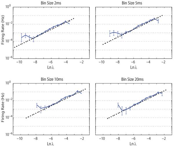
A comparison between an exponential function (dashed) with direct reconstructed estimates of the non-linearity; computed using the raw distribution of Ln λ and the observed spike responses. Ln denotes the natural logarithm operator. The exponential non-linearity employed here represents the probability of observing a spike for each bin. The assumed exponential non-linearity for the model provides a reasonable approximation except at low lambda. Error bars represents the SDs. The vertical (Firing rate) axis is on a logarithmic scale.

2) Prediction rates

Fig. 2 depicts an example for the predicted EMG signals using both the Wiener cascade filter and the SCKF. In this example, EMG envelopes were better predicted using the SCKF (eq. (15)). The SCKF predictions were also smoother than the Wiener cascade filter predictions.

Fig. 2.

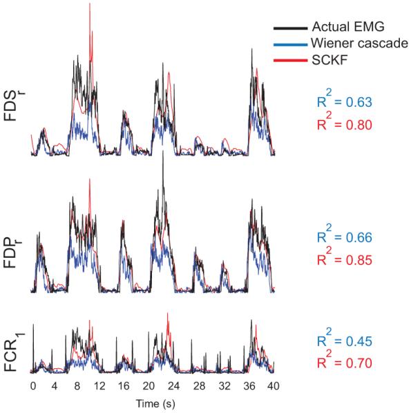
An example of actual (black) and predicted EMG signals using the Wiener cascade filter (blue) and the simplified constrained Kalamn filter (SCKF, red) during the ball-grip task. The R² values were calculated from a 40 second segment of data in this example.

We computed the prediction accuracy of the simplified and full constrained Kalman filter to that of the Wiener cascade filter for four bin sizes within each data file (Fig. 3). On average, the SCKF performance was about 8% higher than the Wiener cascade filter. The prediction difference between the SCKF and the Wiener filter when the bin size was 2 ms was marginally significant (paired t-test: t₁₁ = 2.13, p = 0.056). In order to incorporate the history and coupling components for FCKF, we examined the inter-spike interval (ISI) histograms and empirically concluded that a history window of 20 ms should accommodate enough spikes for each neuron so that the GLM fit would converge. Incorporating the full GLM model further increased the prediction scores by about 4% on average. In the smaller bin sizes, the FCKF predicted the EMG activity more accurately than did the SCKF (e.g. 2 ms bin size: paired t-test: t₁₁ = 4.28, p = 0.001). However this difference diminished when the bin size was 20 ms (paired t-test: t₁₁ = 0.65, p = 0.52). The performance of the constrained Kalman filter estimators increased monotonically when bin size increased.

Fig. 3.

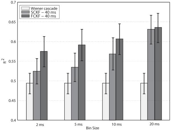
Summary of EMG prediction accuracy with the Wiener cascade, simplified (the generalized linear model without the coupling and history components: eq. (15)), and full constrained Kalman filters (the generalized linear model with the coupling and history components: eq. (12)). Predictions (R² ± S EM) accounted for 49-65% of the variance of the EMGs. The Wiener cascade filter was insensitive to the bin size. However, the prediction accuracy of the constrained Kalman filter improved for larger bin sizes. Including the history and coupling component terms in the GLM improved the prediction rates further. The time delay was set to 40 ms.

3) Bin size, delay, and kernel width

We studied the effect of bin size (4 bin-sizes) and EMG delay lag (3 lags: 20, 40, and 60 ms) on the prediction accuracy of the SCKF using non-overlapping bins. The EMG prediction accuracy was improved by increasing the bin size from 2 ms to 20 ms, Fig. 3. The results for 40 ms delay were slightly higher than the 20 ms and 60 ms delays for all bin sizes.

For the FCKF, we used 20 ms and 40 ms wide rectangular kernels (h_i,j′,j = 1) in (12) and two delay values of 20 ms or 40 ms. For instance, when the bin size and the delay were respectively 5 ms and 40 ms, the rectangular kernel window covered 8 previous data points. Including the history and coupling components improved the prediction results by about 4% on average, when compared to the no kernel (SCKF) condition, at smaller bin sizes of 2 ms and 5 ms. Such an improvement was statistically significant for almost all different configurations. For instance, at 5 ms bin size and 20 ms delay, FCKF (40 ms kernel size) and SCKF prediction scores were 59% and 53%; a 2-tailed t-test across muscles confirms the significance t₁₁ = 4.56, p = 0.001. Such differences diminished with larger bin sizes.

The size of the bins did not influence the performance of the Wiener cascade filter (see Fig. 3). The SCKF and FCKF prediction rates improved monotonically when bin size increase. For large bins the effect of the kernel was smeared irrespective of its size and the SCKF and FCKF results were comparable.

4) Stability

We analyzed the prediction stability of both the Wiener cascade and the constrained Kalman filter over time using the six data files of dataset I in terms of both R² and MS E. We used the filter parameters determined from one data file to predict EMG signals from the remaining data files from either the same or a different day. The predictions used only those neurons that were common to both data files. This included approximately 80-90% of units. The process was carried out for bin sizes of 2 ms, 5 ms, 10 ms, and 20 ms, delay values of 20 and 40 ms. The kernel width for FCKF was set to 40 ms. Fig. 4 and Fig. 5 report the EMG prediction accuracy scores (R² and MS E, respectively) using four different bin sizes.

Fig. 4.

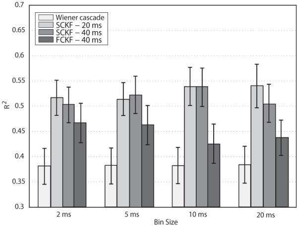
Summary of EMG prediction stability rates (R² ± S EM) using Wiener cascade filter, SCKF (time delay: 20 ms and 40 ms), and FCKF (time delay: 40 ms time delay and kernel width: 40 ms). Predictions accounted for about 55% of the actual EMGs using SCKF, (eq. (15)), and about 45% using FCKF, (eq. (12)). Prediction rates obtained by SCKF were higher than that of the Wiener cascade filter by about 12% on average.

Fig. 5.

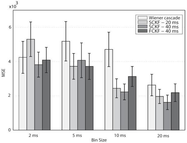
Summary of EMG prediction stability scores (MS E ± S EM) using Wiener cascade filter, SCKF (time delay: 20 ms and 40 ms), and FCKF (time delay: 40 ms time delay and kernel width: 40 ms). The EMG predictions using the proposed filters were closer to the actual EMGs (smaller MSEs) than the predictions of the Wiener cascade filter.

Fig. 4 shows that the SCKF predictions accounted on average 55% of the actual EMGs which was on average 15% more accurate than the Wiener cascade filter. A repeated measures ANOVA was used to test the statistical significance of the differences in prediction rates in terms of R². Tests confirmed the main effect of the predictor (F_1.19,13.08 = 62.67, p < 10⁻⁴). However, the bin size did not influence the prediction scores (F_1.07,18.75 = 1.22, p = 0.31. Post-hoc analysis revealed rates achieved by SCKF (delay 20 ms), SCKF (delay 40 ms), and FCKF (delay 40 ms) were higher than those scored by the Wiener cascade filter (p < 10⁻⁴, p < 10⁻⁴, and p = 0.01, respectively).

Fig. 5 shows that the MS Es between the predicted EMGs and actual EMGs were smaller using the proposed point-process filters specially for larger bin sizes. We used a 4 × 2 ANOVA repeated measures to test the statistical significance of the differences in prediction stability in terms of MS E. Tests revealed that the main effects of type of predictor and bin-size were statistically significant (F_1.74,19.21 = 5.22, p = 0.01 and F_1.25,13.84 = 21.36, p < 10⁻⁴, respectively). Bonferroni corrected post-hoc analysis showed the predictions of the SCKF (delay 40 ms) were marginally more accurate than that of the Wiener cascade filter (p = 0.08).

B. Dataset II

We repeated the analysis for dataset II considering bin sizes of 5, 10, 20, and 50 ms. The mean prediction and stability rates are depicted in Fig. 6. Results show that for this long dataset, prediction rates obtained by the Wiener and Kalman-based filters were comparable (4 × 2 ANOVA repeated measures, n=12, main effect of predictor F_1,11 = 0, p = 0.98).

Fig. 6.

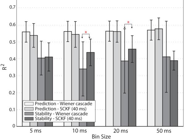
Summary of EMG prediction and stability rates (R² ± S EM) with the Wiener cascade filter and SCKF (eq. (15)) for the large-file dataset. The average R² and their standard error of means for Dataset II are reported. Wiener cascade filter and SCKF results were comparable when large training data was used. Only when the bin sizes were 10 ms and 20 ms the difference in prediction rates were statistically significant, shown with asterisk.

We compared the stability of the Wiener cascade filter and the SCKF (delay 40 ms). When the bin size was 10 ms or 20 ms bin sizes, the SCKF prediction performance was higher than that of the Wiener cascade filter as confirmed by paired t-tests across muscles: at 10 ms t₁₁ = 4.65, p = 0.001 and at 20 ms t₁₁ = 2.69, p = 0.021. Otherwise, the Wiener cascade filter performance matched that of the SCKF.

IV. Concluding Remarks

The ultimate motivation behind this work is to decode attempted muscle activity in paralyzed patients from motor cortical activity and to utilize the decoded signals as a mean to restore motor deficit. To that end, we proposed a non-negatively-constrained point process filter for the prediction of EMG signals from multi-channel spike recordings in M1. We employed the generalized linear model to estimate the instantaneous firing rate of the cells as a function of the EMG activity. This model provided reasonable characterizations between neural activity and motor behavior. Using an optimization interpretation of the conventional Kalman and point-process filters, we accommodated the state non-negativity constraint of the EMG envelopes by the log-barrier method. In the constrained point process filtering setting, the neural non-linear, non-Gaussian, spiking pattern and the inherent non-negative nature of the EMG envelopes were explicitly modeled.

We showed that the GLM could be readily fitted using a few minutes of training data and the constrained point process filter provided reasonably accurate estimates of EMG activity given the instantaneous firing rates of a population of cells in M1. The prediction rates achieved for the SCKF and FCKF were higher than those of the Wiener cascade filter by about 8% and 12%, respectively. In the stability tests, the predictions of the SCKF were about 12% more stable than those of the Wiener cascade filter. The stability scores achieved by the FCKF were on average 5% higher than those given by the Wiener cascade filter. When the amount of training data increased, using the longer data files of dataset II, the constrained point process filter did not achieve consistently better performance rates than the Wiener cascade filter.

The size of the filter parameter space relative to the amount of training data is an important factor in fitting both Wiener- and GLM-based models. The improved performance of the proposed constrained point process filter when compared to the Wiener cascade filter may be due to its smaller number of parameters and compact Bayesian nature. For instance, for prediction of M = 12 EMGs from the activity of C = 100 cells using the proposed filters, one needs to compute C × (M + 1) + 2M² = 1588 parameters (including b_i and ${\mathfrak{B}}_i$ for each neuron, A, and C_q). However, where T denotes the length of the impulse response (in bin), for the same setting the Wiener cascade filter requires T × C × M = 14400 parameters (T = 12 for a bin size of 20 ms and a filter length of 240 ms). Therefore, the Wiener cascade filters suffers dramatically from substantial model overfitting if the training data are limited. It is often recommended to regularize the fitting process by taking into account prior mathematical (e.g. sparsity of the filter) constraints [34]. This can improve the performance of the model when the training data are limited and the feature space is high-dimensional [35] by trading prediction accuracy on the training set for a smoother prediction surface. However, we believe that any gains achieved through the addition of a regularization component to the Wiener-based decoders would transfer, at least partially, to systems using the proposed filters. For instance, in our full GLM setting, for simplicity, we used rectangular history kernels h_i,i’,j and that led to lower performance of the FCKF when compared to the SCKF in the stability test. However, a physiologically-inspired prior for the model would be the temporal smoothness of the history kernels. For example, the raised cosine kernels can provide a fine temporal structure near the time of a spike and a coarse temporal structure at longer delays using a limited number of parameters [22].

In a real-time implementation of the constrained point process filter, the block-tridiagonal structure of H implies that $\widehat{\mathbf{Q}}=-{\mathbf{H}}^{-1}\nabla$ may readily be solved in O(K) time, e.g., by block-Gaussian elimination [36]. One should note that there is no need to compute H⁻¹ explicitly. The matrix formulation of the Kalman filter is equivalent, both mathematically and in terms of computational complexity, to the forward-backward method. Therefore, in contrast to the original Kalman filter, the computation of q_k requires at least a partial forward-backward sweep making the real-time implementation complicated. A potential solution to this problem is suggested in [37]. In addition, in the proposed constrained point process filter, the computational cost incurred in updating H, in each iteration of the Newton optimization and the best tuning of ε in equation (14) have to be taken into account. The Newton’s optimization method converges in only one step [31] for the original linear-Gaussian setting, but for the point process observations, the optimum _1:k is obtained after a few iterations - still of order O(K) time computations. To compute ${\widehat{\mathbf{q}}}_{1:K}^{MAP}$, we initiated the optimization with ε = 0.2 and after few iterations halved the ε in an outer loop. The iteration process stopped if the improvement in the log-likelihood was smaller than an empirical threshold. Further work will be necessary to develop a real-time implementation of the constrained point process filter proposed here.

An alternative way to decrease the computational cost of our algorithm is to reduce the dimension of the observation vector by ranking the neurons with respect to the information they provide and discarding those that are not influential. One such iterative ranking method has been proposed, but it is itself rather complex computationally [32].

Despite the apparent success of the biomimetic BMI, the requirement for training data remains a challenge for ultimate clinical applications with paralysed patients. Motor imagery may provide a suitable substitute for actual movement in patients suffering from cervical spinal cord injury. Hochberg et al. [38] showed that the imagined limb motions modulate neural firing discharge in M1. In their experiment, the paralyzed subject was asked to imagine tracking a cursor on the computer screen that was moved by a technician through a succession of randomly positioned targets - only the cursor and targets were visible on the screen. A linear filter decoder was computed from four minutes of data collected during these imagined movements. Subsequently, the subject used this initial decoder to control movement of a neural cursor. Data generated during these movements were used to update the linear filter estimate. Related approaches have also been used with monkey subjects [39]-[41].

The problem is more complicated in the case of decoding EMG signals, as the idea of imagining the activity of individual muscles is much less intuitive than imagining the kinematics of hand movement. The problem is exacerbated by the high degree of musculoskeletal redundancy of the arm. There are unlimited combinations of muscles by which the same motor output at the fingertips may be achieved which leads to very slow convergence of a decoder and potentially unstable performance. However, muscles exhibit rather stereotyped EMG activity patterns across subjects [42]. Therefore, it might be possible to train an initial filter using “template” EMGs collected from able-bodied subjects during execution of the movements that the patient observes. This initial decoder can then be improved by further mathematical optimization or reinforced via training. Implementing this procedure may be challenging in a clinical environment where collecting enough high quality training data is challenging. In this case, the proposed decoder may play an important role by providing better performance despite limited training data.

In conclusion, we have shown that the constrained point process-based models improve prediction of the envelope of EMG signals from multi-channel neuronal firing rate records with a better stability when the training data are limited. Improvement in the prediction of EMG signals from neural recordings by appropriately regularized Wiener- and Kalman-based filters remains to be studied further.

Appendix I

In a linear-Gaussian setting, (q_1:K, y_1:K) in eq. (2) forms a jointly Gaussian random variable, and therefore the conditional expectation of the hidden state path q_1:k given the observations y_1:k, E(q_1:K|y_1:K) remains Gaussian. Coincidence of the mean and mode of a Gaussian distribution implies that E(q_1:K|y_1:K) is equal to the maximum a posteriori (MAP) estimate of p(q_1:K|y_1:K)

$$\begin{array}{cc}\hfill {\widehat{\mathbf{q}}}_{1:K}& =\arg \underset{{\mathbf{q}}_{1:K}}{\max }p({\mathbf{q}}_{1:K}\mid {\mathbf{y}}_{1:K})=\arg \underset{{\mathbf{q}}_{1:K}}{\max }\log p({\mathbf{q}}_{1:K},{\mathbf{y}}_{1:K})\hfill \\ \hfill & =\arg \underset{{\mathbf{q}}_{1:K}}{\max }\left(\log p\left({\mathbf{q}}_1\right)+\sum _{k=1}^K\log p({\mathbf{q}}_k\mid {\mathbf{q}}_{k-1})+\sum _{k=1}^K\log p({\mathbf{y}}_k\mid {\mathbf{q}}_k)\right)\hfill \\ \hfill & =\arg \underset{{\mathbf{q}}_{1:K}}{\max }\left[-\frac{1}{2}\left({({\mathbf{q}}_1-E\left({\mathbf{q}}_1\right))}^T{\mathbf{C}}_{{\mathbf{q}}_1}^{-1}({\mathbf{q}}_1-E\left({\mathbf{q}}_1\right))+\sum _{k=1}^K{({\mathbf{q}}_k-{\mathbf{Aq}}_{k-1})}^T{\mathbf{C}}_{\mathbf{q}}^{-1}({\mathbf{q}}_k-{\mathbf{Aq}}_{k-1})+\sum _{k=1}^K{({\mathbf{y}}_k-{\mathbf{Bq}}_k)}^T{{\mathbf{C}}_y}^{-1}({\mathbf{q}}_k-{\mathbf{Bq}}_k)\right)\right].\hfill \end{array}$$ (16)

The right-hand-side here is a simple quadratic function in q_1:K. Since p(q_1:K|y_1:K) is Gaussian, that is p(q_1:K|y_1:K) is quadratic, E(q_1:K|y_1:K) may be solved by an unconstrained quadratic program in q_1:k as in equation (4) where the Hessian H matrix is a block-tridiagonal matrix of form

$$\mathbf{H}=\left(\begin{array}{cccccc}\hfill {\mathbf{D}}_1\hfill & \hfill {\mathbf{R}}_{1,2}\hfill & \hfill 0\hfill & \hfill \cdots \hfill & \hfill \cdots \hfill & \hfill 0\hfill \\ \hfill {\mathbf{R}}_{2,1}\hfill & \hfill {\mathbf{D}}_2\hfill & \hfill {\mathbf{R}}_{2,3}\hfill & \hfill 0\hfill & \hfill \cdots \hfill & \hfill ⋮\hfill \\ \hfill 0\hfill & \hfill {\mathbf{R}}_{k+1,k}\hfill & \hfill {\mathbf{D}}_k\hfill & \hfill {\mathbf{R}}_{k,k+1}\hfill & \hfill \cdots \hfill & \hfill ⋮\hfill \\ \hfill ⋮\hfill & \hfill \ddots \hfill & \hfill \ddots \hfill & \hfill \ddots \hfill & \hfill \cdots \hfill & \hfill 0\hfill \\ \hfill 0\hfill & \hfill \cdots \hfill & \hfill \cdots \hfill & \hfill \cdots \hfill & \hfill {\mathbf{D}}_{K-1,K-1}\hfill & \hfill {\mathbf{R}}_{K-1},K\hfill \\ \hfill 0\hfill & \hfill \cdots \hfill & \hfill \cdots \hfill & \hfill \cdots \hfill & \hfill {\mathbf{R}}_{K,K-1}\hfill & \hfill {\mathbf{D}}_K\hfill \end{array}\right)$$ (17)

and its elements may be computed (for k = 1, 2, … , K) with

$$\begin{array}{cc}\hfill {\mathbf{D}}_k& =\frac{{\partial }^2}{\partial {\mathbf{q}}_k^2}\log p({\mathbf{y}}_k\mid {\mathbf{q}}_k)+\frac{{\partial }^2}{\partial {\mathbf{q}}_k^2}\log p({\mathbf{q}}_k\mid {\mathbf{q}}_{k-1})+\frac{{\partial }^2}{\partial {\mathbf{q}}_k^2}\log p({\mathbf{q}}_{k+1}\mid {\mathbf{q}}_k),\hfill \\ \hfill {\mathbf{R}}_{k,k+1}& ={\mathbf{R}}_{k+1,k}^T=\frac{{\partial }^2}{\partial {\mathbf{q}}_k\partial {\mathbf{q}}_{k+1}}\log p({\mathbf{q}}_{k+1}\mid {\mathbf{q}}_k).\hfill \end{array}$$ (18)

For instance, ${\mathbf{D}}_1=-\left({\mathbf{C}}_{{\mathbf{q}}_1}^{-1}+{\mathbf{A}}^T{\mathbf{C}}_{\mathbf{q}}\mathbf{A}+{\mathbf{B}}^T{\mathbf{C}}_y^{-1}\right)$ and ${\mathbf{R}}_{2,1}={\mathbf{C}}_{\mathbf{q}}^{-1}{\mathbf{A}}^T$. In (4) is a vector in which the i-th element is

$$\begin{array}{cc}\hfill {\nabla }_k& =\frac{\partial \log p({\mathbf{q}}_{1:K}\mid {\mathbf{y}}_{1:K})}{\partial {\mathbf{q}}_k}\hfill \\ \hfill & =-{\mathbf{C}}_{\mathbf{q}}^{-1}({\mathbf{q}}_k-{\mathbf{Aq}}_{k-1})+{\mathbf{A}}^T{\mathbf{C}}_q^{-1}({\mathbf{q}}_{k+1}-{\mathbf{Aq}}_k)+{\mathbf{B}}^T{\mathbf{C}}_y^{-1}({\mathbf{y}}_k-{\mathbf{Bq}}_k).\hfill \end{array}$$ (19)

Appendix II

The first and second derivatives of log p(y_k|q_k) are

$$\frac{\partial \log p({\mathbf{y}}_k\mid {\mathbf{q}}_k)}{\partial {\mathbf{q}}_k}=\sum _{i=1}^C\left(\Delta N_k^i-{\lambda }_k^i\Delta t_k\right){\mathfrak{B}}_i,$$ (20)

$$\frac{{\partial }^2\log p({\mathbf{y}}_k\mid {\mathbf{q}}_k)}{\partial {\mathbf{q}}_k^2}=\sum _{i=1}^C-{\lambda }_k^i\Delta t_k{\mathfrak{B}}_i^T{\mathfrak{B}}_i.$$ (21)

Equation (21) demonstrates directly that log p(y_k|q_k) is concave since ${\lambda }_k^i\ge 0$.

References

- [1].Fagg AH, Hatsopoulos NG, de Lafuente V, Moxon KA, Nemati S, Rebesco JM, Romo R, Solla SA, Reimer J, Tkach D, Pohlmeyer EA, Miller LE. Biomimetic brain machine interfaces for the control of movement. J. Neurosci. 2007;27(44):11842–11846. doi: 10.1523/JNEUROSCI.3516-07.2007. [DOI] [PMC free article] [PubMed] [Google Scholar]
- [2].Nazarpour K, Jackson A. Biomimetic and biofeedback approaches for brain machine interface; Proc. APSIPA ASC, Biopolis; Singapore. 2010. [Google Scholar]
- [3].Schwartz AB. Direct cortical representation of drawing. Science. 1994;265:540–542. doi: 10.1126/science.8036499. [DOI] [PubMed] [Google Scholar]
- [4].Serruya MD, Hatsopoulos NG, Paninski L, Fellows MR, Donoghue JP. Instant neural control of a movement signal. Nature. 2008;416:141–142. doi: 10.1038/416141a. [DOI] [PubMed] [Google Scholar]
- [5].Wessberg J, Stambaugh CR, Kralik JD, Beck PD, Laubach M, Chapin JK, Kim J, Biggs SJ, Srinivasan MA, Nicolelis MA. Real-time prediction of hand trajectory by ensembles of cortical neurons in primates. Nature. 2000;408:361–365. doi: 10.1038/35042582. [DOI] [PubMed] [Google Scholar]
- [6].Georgopoulos AP, Ashe J, Smyrnis N, Taira M. The motor cortex and the coding of force. Science. 1992;256:1692–1695. doi: 10.1126/science.256.5064.1692. [DOI] [PubMed] [Google Scholar]
- [7].Evarts EV. Relation of pyramidal tract activity to force exerted during volumeuntary movement. J. Neurophysiol. 1968;31:14–27. doi: 10.1152/jn.1968.31.1.14. [DOI] [PubMed] [Google Scholar]
- [8].Morrow MM, Jordan LR, Miller LE. Direct comparison of the task-dependent discharge of M1 in hand space and muscle space. J. Neurophysiol. 2007;97:1786–1798. doi: 10.1152/jn.00150.2006. [DOI] [PMC free article] [PubMed] [Google Scholar]
- [9].Sergio LE, Hamel-Paquet C, Kalaska JF. Motor cortex neural correlates of output kinematics and kinetics during isometric-force and arm-reaching tasks. J. Neurophysiol. 2005;94:2353–2378. doi: 10.1152/jn.00989.2004. [DOI] [PubMed] [Google Scholar]
- [10].Rivera-Alvidrez Z, Kalmar RS, Ryu SI, Shenoy KV. Low dimensional neural features predict muscle emg signals. Proc. IEEE EMBC. 2010:6027–6033. doi: 10.1109/IEMBS.2010.5627604. [DOI] [PubMed] [Google Scholar]
- [11].Townsend B, Paninski L, Lemon R. Linear encoding of muscle activity in primary motor cortex and cerebellum. J. Neurophys. 2006;96:2578–2592. doi: 10.1152/jn.01086.2005. [DOI] [PubMed] [Google Scholar]
- [12].Carmena JM, Lebedev MA, Crist RE, O’Doherty JE, Santucci DM, Dimitrov DF, Patil PG, Henriquez CS, Nicolelis MAL. Learning to control a brainmachine interface for reaching and grasping by primates. PLoS Biol. 2003;1:e42. doi: 10.1371/journal.pbio.0000042. [DOI] [PMC free article] [PubMed] [Google Scholar]
- [13].Pohlmeyer EA, Solla SA, Perreault EJ, Miller LE. Prediction of upper limb muscle activity from motor cortical discharge during reaching. J. Neural Eng. 2007;4:369–379. doi: 10.1088/1741-2560/4/4/003. [DOI] [PMC free article] [PubMed] [Google Scholar]
- [14].Oby ER, Ethier C, Bauman M, Perreault EJ, Ko J, Miller LE. Statistical Signal Processing for Neuroscience and Neurotechnology. Academic Press; Elsevier: 2010. Getting a grip on spinal cord injury: A novel application of a Brain Machine Interface; pp. 369–406. [Google Scholar]
- [15].Pohlmeyer EA, Oby ER, Perreault EJ, Solla SA, Kilgore KL, Kirsch RF, Miller LE. Toward the restoration of hand use to a paralyzed monkey: Brain-controlled functional electrical stimulation of forearm muscles. PLoS ONE. 2009;4:1–8. doi: 10.1371/journal.pone.0005924. [DOI] [PMC free article] [PubMed] [Google Scholar]
- [16].Stevenson IH, Rebesco JM, Miller LE, Körding KP. Inferring functional connections between neurons. Curr. Opin. NeuroBiol. 2008;18:582–588. doi: 10.1016/j.conb.2008.11.005. [DOI] [PMC free article] [PubMed] [Google Scholar]
- [17].Wu W, Gao Y, Bienestock E, Donoghue JP, Black MJ. Bayesian papulation decoding of motor cortical activity using a Kalman filter. Neural Computation. 2006;18(1):80–118. doi: 10.1162/089976606774841585. [DOI] [PubMed] [Google Scholar]
- [18].Kulkarni JE, Paninski L. State-space decoding of goal-directred movements. IEEE Sig. Process. Mag. 2008;25:78–86. [Google Scholar]
- [19].Wu W, Kulkarni JE, Hatsopoulos NG, Paninski L. Neural decoding of hand motion using a linear state-space model with hidden states. IEEE Trans. Neural Syst. Rehabil. Eng. 2009;17(4):370–378. doi: 10.1109/TNSRE.2009.2023307. [DOI] [PMC free article] [PubMed] [Google Scholar]
- [20].Lawhern V, Wu W, Hatsopoulos N, Paninski L. Population decoding of motor cortical activity using a generalized linear model with hidden states. J. Neurosci. Meth. 2010;189:267–280. doi: 10.1016/j.jneumeth.2010.03.024. [DOI] [PMC free article] [PubMed] [Google Scholar]
- [21].Truccolo W, Eden UT, Fellows MR, Donoghue JP, Brown EN. A point process framework for relating neural spiking activity to spiking history, neural ensemble, and extrinsic covariate effects. J. Neurophysiol. 2005;93:1074–1089. doi: 10.1152/jn.00697.2004. [DOI] [PubMed] [Google Scholar]
- [22].Pillow J, Shlens J, Paninski L, Sher A, Litke A, Chichilnisky E, Simoncelli E. Spatiotemporal correlations and visual signaling in a complete neuronal population. Nature. 2008;454:995–999. doi: 10.1038/nature07140. [DOI] [PMC free article] [PubMed] [Google Scholar]
- [23].Durbin J, Koopman S. Time Series Analysis by State Space Method. Oxford University Press; 2001. [Google Scholar]
- [24].Fahrmeir L, Tutz G. Multivariate Statistical Modelling Based on Generalized Linear Models. Springer; 1994. [Google Scholar]
- [25].Brockwell AE, Rojas AL, Kass RE. Recursive bayesian decoding of motor cortical signals by particle filtering. J. Neurophysiol. 2004;91:1899–1907. doi: 10.1152/jn.00438.2003. [DOI] [PubMed] [Google Scholar]
- [26].Koyama S, Paninski L. Efficient computation of the maximum a posteriori path and parameter estimation in integrate-and-fire and more general state-space models. J. Comput. Neurosci. 2009;29:89–105. doi: 10.1007/s10827-009-0150-x. [DOI] [PubMed] [Google Scholar]
- [27].Paninski L. Maximum likelihood estimation of cascade point-process neural encoding models. Network:Computations in Neural Sys. 2004;15:243–262. [PubMed] [Google Scholar]
- [28].Dennis JE, Schnabel RB. Numerical Methods for Unconstrained Optimization and Nonlinear Equations. SIAM Publications; Philadelphia: 1996. [Google Scholar]
- [29].Paninski L, Fellows MR, Hatsopoulos NG, Donoghue JP. Spatiotemporal tuning of motor cortical neurons for hand position and velocity. J. Neurophusiol. 2004;91:515–532. doi: 10.1152/jn.00587.2002. [DOI] [PubMed] [Google Scholar]
- [30].Bella BM, Burkeb JV, Pillonetto G. An inequality constrained nonlinear KalmanBucy smoother by interior point likelihood maximization. Automatica. 2009;45:25–33. [Google Scholar]
- [31].Paninski L, Ahmadian Y, Ferreira DG, Koyama S, Rahnama Rad K, Vidne M, Vogelstein J, Wu W. A new look at state-space models for neural data. J. Comput. Neurosci. 2009;29:107–126. doi: 10.1007/s10827-009-0179-x. [DOI] [PMC free article] [PubMed] [Google Scholar]
- [32].Westwick DT, Pohlmeyer EA, Solla SA, Miller LE, Perreault EJ. Identification of multiple-input systems with highly coupled inputs: application to EMG prediction from multiple intracortical electrodes. Neural Computation. 2006;18(2):329–355. doi: 10.1162/089976606775093855. [DOI] [PMC free article] [PubMed] [Google Scholar]
- [33].Chichilnisky EJ. A simple white noise analysis of neuronal light responses. Network. 2001;12:199–213. [PubMed] [Google Scholar]
- [34].Tibshirani R, Saunders M, Rosset S, Zhu J, Knight K. Sparsity and smoothness via the fused lasso. J. Roy. Soc. B. 2005;67:91–108. [Google Scholar]
- [35].Björck A. Numerical methods for least squares problems. SIAM; 1996. [Google Scholar]
- [36].Press W, Teukolsky S, Vetterling W, Flannery B. Numerical recipes in C. Cambridge University Press; 1992. [Google Scholar]
- [37].Ahmadian Y, Packer AM, Yuste R, Paninski L. Designing optimal stimuli to control neuronal spike timing. 2011 doi: 10.1152/jn.00427.2010. Under review: available online in http://www.stat.columbia.edu/~liam/research/pubs/yasharoptcont.pdf. [DOI] [PMC free article] [PubMed]
- [38].Hochberg LR, Serruya MD, Friehs GM, Mukand JA, Saleh M, Caplan AH, Branner A, Chen D, Penn RD, Donoghue JP. Neuronal ensemble control of prosthetic devices by a human with tetraplegia. Nature. 2006;442(7099):164–171. doi: 10.1038/nature04970. [DOI] [PubMed] [Google Scholar]
- [39].Velliste M, Perel S, Spalding MC, Whitford AS, Schwartz AB. Cortical control of a prosthetic arm for self-feeding. Nature. 2008;453:1098–1101. doi: 10.1038/nature06996. [DOI] [PubMed] [Google Scholar]
- [40].Wahnoun R, He J, Tillery SIH. Selection and parameterization of cortical neurons for neuroprosthetic control. J. Neural Eng. 2006;3:162–171. doi: 10.1088/1741-2560/3/2/010. [DOI] [PubMed] [Google Scholar]
- [41].Tkach D, Reimer J, Hatsopoulos N. Congruent activity during action and action observation in motor cortex. J. Neurosci. 2007;27:13241–13250. doi: 10.1523/JNEUROSCI.2895-07.2007. [DOI] [PMC free article] [PubMed] [Google Scholar]
- [42].Hallett M, Shahani BT, Young RR. EMG analysis of stereotyped voluntary movements in man. J. Neurol. Neurosurg. Psych. 1975;38:1154–1162. doi: 10.1136/jnnp.38.12.1154. [DOI] [PMC free article] [PubMed] [Google Scholar]