

Abstract
Motivation: Low coverage sequencing provides an economic strategy for whole genome sequencing. When sequencing a set of individuals, genotype calling can be challenging due to low sequencing coverage. Linkage disequilibrium (LD) based refinement of genotyping calling is essential to improve the accuracy. Current LD-based methods use read counts or genotype likelihoods at individual potential polymorphic sites (PPSs). Reads that span multiple PPSs (jumping reads) can provide additional haplotype information overlooked by current methods.
Results: In this article, we introduce a new Hidden Markov Model (HMM)-based method that can take into account jumping reads information across adjacent PPSs and implement it in the HapSeq program. Our method extends the HMM in Thunder and explicitly models jumping reads information as emission probabilities conditional on the states of adjacent PPSs. Our simulation results show that, compared to Thunder, HapSeq reduces the genotyping error rate by 30%, from 0.86% to 0.60%. The results from the 1000 Genomes Project show that HapSeq reduces the genotyping error rate by 12 and 9%, from 2.24% and 2.76% to 1.97% and 2.50% for individuals with European and African ancestry, respectively. We expect our program can improve genotyping qualities of the large number of ongoing and planned whole genome sequencing projects.
Contact: dzhi@ms.soph.uab.edu; kzhang@ms.soph.uab.edu
Availability: The software package HapSeq and its manual can be found and downloaded at www.ssg.uab.edu/hapseq/.
Supplementary information: Supplementary data are available at Bioinformatics online.
1 INTRODUCTION
Recent advances in array-based genotyping technologies and the detailed catalog of genetic variants from the HapMap project have enabled genome-wide association studies (GWAS) to successfully identify hundreds of common genetic variants that are associated with common human diseases (Altshuler et al., 2008; Hirschhorn, 2009; Manolio et al., 2009). However, majority of those common variants only explain a small proportion of the estimated heritability of common diseases. Therefore, efforts are turning to identify other factors, including rare genetic variants that may account for the missing heritability of common diseases (Maher, 2008; Manolio et al., 2009; McCarthy et al., 2008). Although array-based genotyping technologies can genotype previously identified variants, they are ineffective to identify novel rare variants across the human genome. Recent advances in next-generation sequencing (NGS) technologies provide an affordable way to capture both common and rare variants effectively (Bentley et al., 2008; Metzker, 2010; Pushkarev et al., 2009). Indeed, low coverage sequencing has already been adopted by the 1000 Genomes Project (Durbin et al., 2010) aiming to establish an unprecedented comprehensive catalog of human genetic variants in multiple populations. Due to plummeting sequencing costs, whole genome sequencing is becoming increasingly practically affordable in genetic association studies of complex human diseases where hundreds or thousands individuals are sequenced. We predict that a flood of sequencing data will soon be available for genetic researchers.
The meaningful analysis of NGS data depends crucially on the accurate genotype calling. Essentially, NGS technologies randomly fragment the whole genome (or targeted regions of the genome) for a number of individuals and generate short reads, typically 30–200 bp in length, which are then mapped back to a reference genome. Often, ‘SNP calling’ refers to the identification of potential polymorphic sites (PPSs), while ‘genotype calling’ refers to the determination of actual genotype for each individual at each PPS (Nielsen et al., 2011). While these two tasks are not as clearly separated in sequencing-based as in array-based genotyping, genotype calling methods typically rely on a set of preliminary single nucleotide polymorphism (SNP) calls and infer genotypes based on the counts and qualities of reads covering PPSs carrying the reference and alternative alleles. Unlike array-based genotyping technologies that read out image intensities at each site probed, sequencing-based genotyping methods typically start with counts of reads carrying the reference allele or an alternative allele, or an inferred genotype likelihood, at each PPS. Although the raw sequencing error rates of individual reads are about 0.5–1.0% (Metzker, 2010), these errors can accumulate when we are looking at billions of positions across the genome. Moreover, due to the randomly sampling nature of shotgun sequencing, some genomic regions may be covered by very few reads or even no reads—this problem is especially severe when dealing with low coverage sequencing data.
Several methods have been developed for genotyping calling. Early methods generally consider the counts at each PPS for each individual separately thus ignoring the linkage disequilibrium (LD) between nearby PPSs (Li et al., 2008, 2009b). It has been shown that such methods work well with high coverage sequencing data, but have lower power and higher error rates for low coverage data (Bentley et al., 2008; Wendl and Wilson, 2008). For example, Bentley et al. (2008) reported an accuracy of 99% with 30× coverage, Le and Durbin (2010) applied SAMtools (Li et al., 2009a) to 100 samples of 4× coverage and found that the genotype error rate can be as high as 28% for heterozygous sites. Therefore, newer methods that utilize the LD among nearby PPSs are developed (Browning and Yu, 2009; Duitama et al., 2011; Le and Durbin, 2010; Li et al., 2010). Although the specific models used in LD-based methods for genotype calling from NGS data are different, their underlying principle is the same: short segments of chromosome (haplotypes) are shared among individuals due to the LD so the genotype at nearby PPSs can be used to infer genotypes at the PPS of interest. LD-based methods achieve high accuracy for genotype calling with low coverage sequencing data: Li et al. (2011) reported that their Hidden Markov Model (HMM) implemented in Thunder has an accuracy of >98% for genotype calling with 4× coverage data. Nielsen et al. (2011) compared the GATK Unified Genotyper (DePristo et al., 2011; McKenna et al., 2010) and the LD-based method Beagle (Browning and Yu, 2009) and found that the use of LD information greatly improved the accuracy for genotype calling: Beagle has an accuracy of 96%, whereas GATK has an accuracy of 87% for high call rates.
An important piece of source of haplotype information is ignored by existing LD-based genotype calling methods: the haplotype information within individual reads. For example, we observe a read having allele A at the PPS j and B at the PPS j+1, we know that one of haplotypes of that individual is likely to be AB across PPSs j and j+1. Existing methods essentially ‘break’ the haplotype information of multiple PPSs covered by a single read and only use counts observed at each PPS separately. One may argue that most NGS technologies generate ‘short’ reads and thus it is unlikely that a read will span more than one PPS and thus haplotypes within individual reads may not offer much information. We have the following reasons supporting the use of such haplotype information. First, with the rapid advances of NGS technologies, new version of these technologies can generate longer reads, thus the haplotype information provided by these reads can be substantial and used to improve the accuracy for genotype calling. Second, many new NGS technologies can generate ‘paired end’ reads, which means both ends of a DNA segment are sequenced. Apparently paired end reads provide the long range haplotype information over PPSs. Third, although the density of true polymorphic sites may not be high, genotype calling algorithms will be working on a set of PPSs made by a preliminary SNP caller that may contain false positives, i.e. falsely reported PPSs that are actually monomorphic. Haplotype information in reads covering more than one PPS will be useful for genotype calling.
In this work, we introduce a new HMM that extends the Thunder HMM of Li et al. (2010) to incorporate such haplotype information in reads that cover two or more adjacent PPSs. We derive probability calculations to have similar computational efficiency as Thunder. We compare our method with Thunder through extensive simulations and real sequencing data from the 1000 Genomes Project. Our simulation and real data analyses show that our method outperforms the Thunder method in terms of accuracy for genotyping calling in many practical settings of sequencing experiments.
2 METHODS
2.1 Notations
For shotgun sequencing or other single molecular sequencing technologies, we observe the counts at L PPSs for K individuals. Throughout, we assume the makers are biallelic SNPs, with alleles labeled as A and B. We denote Clk=(Alk, Blk)(l=1,…, L and k=1,…, K) as the number of alleles A and B that are observed at the PPS l for the individual k from the reads that cover a single PPS or multiple non-adjacent PPSs. Note that the both Alk and Blk can be zero if some PPSs are not covered by reads. We denote Rlk=(nAA,lk, nAB,lk, nBA,lk, nBB,lk) is the number of combinations of bases A and B across the PPSs l and l−1 for the individual k that are simultaneously observed in a single read. In this article, we only consider such data from two adjacent PPSs. We remark that R and C=(A, B) represent non-overlapping information. We denote Glk as the underlying genotype at the PPS l for the individual k, which is not observed and will be inferred on the basis of Clk and Rlk.
For the HMM implemented in Thunder (Li et al., 2010), it assumes there are H template haplotypes and each of them is sequenced at L PPSs. We use a series of indicator variables S1k,…, SLk(k=1,…, K) to represent a hypothetical (and unobserved) state sequence for the individual k, indicating to which template haplotypes the individual k is closest at the PPS l. At a specific PPS l, diploid state Slk=(xlk, ylk) indicates that the two haplotypes of the individual k are xlk and ylk out of the H template haplotypes, respectively. For genotype imputation, both external haplotypes (e.g. haplotypes obtained from the external reference data such as data from the HapMap Project) and/or internal haplotypes (haplotypes estimated from sequenced individuals in the same study sample) can be used as template haplotypes (Li et al., 2010; Marchini et al., 2007). For NGS data, external haplotype templates are often incomplete and/or unavailable. As a result, Thunder often uses internal haplotype templates only. For K individuals, the number of internal template haplotypes is 2(K−1) and the template haplotypes themselves are different across different individuals. For the rest of article, we will ignore the individual index superscript k for the sake of simplifying notations. This is fine because our algorithm runs in a Gibbs sampler fashion and iteratively infers the genotypes and the underlying states for each individual given the template haplotypes of the rest of the individuals.
2.2 The HMM for the whole genome shotgun sequencing data in Thunder
The HMM in Thunder (Li et al., 2010) can be described as following:
In the model, P(S1 ) denotes the prior probability of the initial state and is usually assumed to be equal for all possible compatible haplotype configurations of each individual, P(Sl|Sl−1) denotes the transition probability between two states and reflects the likelihood of historical recombination events between the PPSs l and l−1, P(Cl=(Al, Bl)|Sl) denotes the emission probability, which is the probability of observed counts conditioning on the underlying state at the PPS l. It is worth noting that Al and Bl are the observed numbers alleles A and B at the PPS l from all reads.
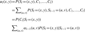
The genotyping inference algorithm is basically a Gibbs sampler: a random pair of haplotypes of each individual is assigned according to the observed counts data. Then, S1,···, SL for each individual k are sampled separately according to the likelihood function L(S| C)∝P(C, S). Specifically, SL is first sampled according to P(C, S), then Sl (l=L−1,…, 1) are sampled according to the following conditional probability:
where P(Sl=(xl, yl), C1,…, Cl) is the forward probability and can be efficiently calculated through Baum's forward algorithm (Baum, 1972). Then S1,…, SL are used to impute genotype G1,…, GL of that individual according to P(Cl=(Al, Bl)|Sl) and determine the new pair of haplotypes of that individual. Then new pair of haplotypes replaces the old pair of haplotypes and is used as the template haplotypes for other individuals. The sampling procedure is performed over all individuals and repeated for a number of times (e.g. 50–100). The consensus genotype and pair of haplotypes of each individual can then be determined by averaging results over repeats.
It is worth mentioning the calculation of the forward probability here. The forward probability can be calculated as following:
 |
Note that the summation over all H2 states and the overall complexity of calculation can be O(H4) without the simplification. As we have mentioned that the HMM often uses H=2(K−1) internal template haplotypes, the direct calculation can be time consuming. However, the transition probability, P(Sl=(x, y)|Sl−1=(u, v)), only depends on if there is a recombination between Sl and Sl−1. Therefore, the calculation can be simplified so that the complexity of the computation is O(H2) rather than O(H4) (Li et al., 2010).
2.3 Extended HMM with the incorporation of haplotype information from reads
We extended the HMM in Thunder by incorporating the haplotype information of jumping reads and implemented it in the HapSeq program. Essentially, the proposed HMM in HapSeq can be defined as following:
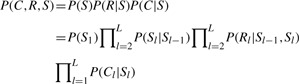 |
Here C and R are non-overlapping and independent because they are from reads that cover only one PPS and reads that cover two adjacent PPSs, respectively. There is one major difference between this HMM and the HMM implemented in MaCH and Thunder. This HMM uses a separate emission probability term, P(Rl|Sl−1, Sl), to model the jumping read information (Fig. 1). P(Rl|Sl−1, Sl) is the probability of observed number of jumping reads conditioning on the underlying state at the PPSs l−1 and l. Note that the emission probability P(Rl|Sl−1, Sl) not only depends on Sl but also Sl−1 because Rl actually is the observed number of haplotypes across the PPSs l−1 and l.
Fig. 1.

Schematic illustration of the HMM in Thunder and HapSeq. For the HMM in Thunder, there is only one term for the emission probability, P(Cl|Sl). For the HMM in HapSeq, an additional emission probability term, P(Rl|Sl−1, Sl), is used to model the jumping read information.
Once the prior probability [P(S1)], the transition probability [P(Sl|Sl−1)] and the emission probability [P(Cl|Sl) and P(Rl|Sl−1, Sl)] are defined (please refer to Section 2.4 for details), we can use the same Monte-Carlo procedure used in MaCH and Thunder to sample S1,…, SL, impute the genotype and determine the pair of haplotypes of each individual. Here we just describe the procedure to sample S1,…, SL. SL is first sampled according to P(C, R, S), then Sl(l=L−1,…, 1) are sampled according to the following conditional probability:
 |
where αl(x, y)=P(Sl=(x, y), C1,…, Cl, R2,…, Rl) is the forward probability and can be efficiently calculated through Baum's forward algorithm. Again, the calculation can be simplified so that the complexity of the computation is O(H2) rather than O(H4) when only the internal haplotype template is used (please refer to Section 2.5 for more details).
2.4 Formulas used in the HMM in HapSeq
We further denote Tl(i)(l=1,…, L and i=1,…, H) as the allele observed at PPS l in the template haplotype i, so Tl(Slk)={Tl(xlk), Tl(ylk)} is the observed genotype at the PPS l for the individual k given the underlying hidden state Slk.
The prior probability, P(S1), is assumed to be equal for all possible compatible haplotype configurations of each individual. This definition is the same as the definition in MaCH and Thunder (Li et al., 2010).
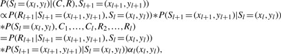
The transition probability, P(Sl|Sl−1), is also the same as that is defined in MaCH and Thunder (Li et al., 2010). Specifically, the transition probability is defined as a function of the crossover parameter θl:
 |
The emission probability, P(Cl=(Al, Bl)|Sl), is the same as that is defined in MaCH and Thunder (Li et al., 2010) as well. Specifically, the emission probability is the summation over all possible genotypes of Gl(A/A, A/B, B/B):
P(Gl|Sl) is the emission probability of an observed genotype and is defined as a function of the error parameter εl:
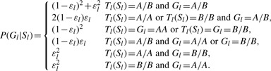 |
The error parameter εl reflects the combined effect of gene conversion, mutation and genotyping error.
P(Cl=(Al, Bl)|Sl) is defined as a function of the error parameter δ:
The error parameter δ reflects the per base sequencing error rate and can be separated from the effect of mutation and gene conversion captured by εl (Li et al., 2010).
The emission probability, P(Rl|Sl−1, Sl) is based on two haplotypes h1l and h2l defined by Sl−1 and Sl across the PPSs l−1 and l and the error parameter δ , in which the error parameter δ is the same as in P(Al, Bl|Sl) and reflects the per base sequencing error rate. Specifically, P(Rl|Sl−1, Sl) is defined to follow a multi-nominal distribution:
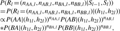 |
where
and
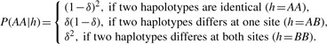 |
P(AB|(h1l, h2l)), P(BA|(h1l, h2l) and P(BB|(h1l, h2l) can be defined similarly.
2.5 The algorithm for the efficient calculation of forward probabilities
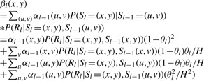
First, we define the following forward probability, αl(x, y)=P(Sl=(x, y), C1,…, Cl, R2,…, Rl), the joint probability of hidden state Sl and observed C=(A, B), and R from the PPSs 1 to l, then:
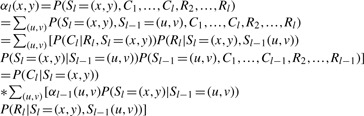 |
From this formula, we first write it out according to the transition probability, P(Sl=(x, y)|Sl−1=(u, v)) and notice that this probability actually only depends on if there is a recombination between Sl and Sl−1:
 |
We further define the following quantity:
And notice that P(Rl|Sl=(x, y), Sl−1(x, v)) is a function of alleles observed at PPS j for the template haplotypes x and y and alleles observed at PPS j−1 for the template haplotypes x and v. Specifically, P(Rl|Sl=(x, y), Sl−1(x, y)) is a function of Tl(Sl=(x, y))={Tl(x), Tl(y)} and Tl−1(Sl−1=(x, v))={Tl−1(x), Tl−1(v)}. Since Tl(y) can only take two possible values: A and B, we only need to calculate two different Dl(x, y). In summary, we can define:
Similarly, we can define:
and
These quantities only need to be calculated once before each of αl(x, y) and βl(x, y) are calculated and the overall complexity of such computation is O(H2), where H is the number of template haplotypes. In summary, the forward probability can be calculated as following:
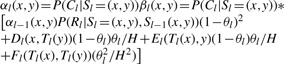 |
with an overall computational complexity of O(H2) instead of O(H4).
2.6 Simulation settings
We used simulated sequencing data to assess the performance of Thunder and HapSeq. We first generated 3000 chromosomes, each of length 100 kb, using the cosi program (Schaffner et al., 2005) that is based on a coalescent model, the ‘European population’ in the ‘bestfit’ model distributed with the cosi package, taking into account the HapMap LD patterns, local recombination rates and recent human population demography. We then generated 16 sets of chromosomes, representing all combinations of sample sizes (K=60 or K=100), read lengths (36 or 75 bp), sequencing error rates (0.2 or 0.5%) and paired end setting (‘paired’ or ‘unpaired’).
For each set, we generated sequencing reads of 4× coverage. Read starting positions were placed uniformly randomly along the chromosome, and sequencing errors were generated uniformly randomly along the length of the reads as well. For paired end settings, we assumed an ‘insert fragment’ length of 200 bp. The starting positions of insert fragments were placed uniformly randomly along the chromosome, and a pair of reads from each end of the insert fragment was generated. Our simulation did not incorporate biases in real sequencing data such as read starting position preferences, sequencing error biases and variations of insert fragment lengths.
Because of the large number of sites probed and the sequencing error rates, many non-polymorphic sites may harbor one or more bases other than the reference. To focus time-consuming LD-based analyses on likely polymorphic sites, genotype calling algorithms typically first promote polymorphic sites with reads carrying different alleles, designated as ‘potential polymorphic sites’. There is a practical decision as to what are the optimal site promotion criteria. Strict criteria will purge out false positive polymorphic sites and thus lower the computational cost, but also run the risk of eliminating true polymorphic sites. On the other hand, lenient criteria will keep more true polymorphic sites, but with a higher computational cost for genotype calling. We followed Li et al. (2010) and calculated the score  , where ck is the minor allele count of individual k at each site. We promoted sites with w≥5 for K=60 and w≥7 for K=100. We ran Thunder and HapSeq to these sites with 10 different random seeds and used the internal haplotype template. The average genotypic discordance rate, the percentage of imputed genotypes that are inconsistent with the true genotypes and the average switch error which is defined as number of switches between the original haplotype and the reconstructed haplotype, are used as criteria to quantify the performance of Thunder and HapSeq.
2.7 Evaluation using the 1000 Genomes Project pilot data
Simulations may not be able to capture all complexities arose from real sequencing data. Therefore, we evaluated Thunder and HapSeq using the 1000 Genomes Project pilot data. The low-coverage pilot data of chromosome 20 are downloaded for 47 individuals of Utah residents with Northern and Western European ancestry from the CEPH collection (CEU) and 52 individuals of Yoruba in Ibadan of Nigeria (YRI) from http://www.1000genomes.org/. We used the polymorphic sites (but not the genotypes) defined in the VCF files (1000G-PS) and then an internal perl script to parse the BAM files for each individual to obtain the read counts and jumping reads information at these sites. We ran both Thunder and HapSeq and compared the estimated genotypes against the corresponding genotypes that are available in the HapMap project. A more detailed description of the evaluation process can be found in the Supplementary Material.
3 RESULTS
3.1 Overall results from simulations
Across 16 simulation settings, the average genotypic discordance rates of HapSeq and Thunder are 0.60 and 0.86%, respectively (Table 1 and Fig. 2). In other words, HapSeq makes 30% less genotypic errors than Thunder. For each simulation setting, the P-value was calculated using the t-test across 10 runs with different random seeds. For 13 simulation settings, HapSeq has a smaller number of discordant genotypes than Thunder in each run and HapSeq performs significantly better than Thunder with the P < 0.05. For 2 simulation settings, both with the read length of 36 bp, in average HapSeq has less number of discordant genotypes than Thunder but has larger number of discordant genotypes than Thunder in some runs. For the setting with the sample size of 100, the sequencing error rate of 0.2%, and the read length of 36 bp, Thunder outperforms HapSeq for 0.001% in terms of genotypic discordance rate. This may be due to the small percentage of jumping reads from shorter reads and the higher power of larger sample size. In terms of switch error, HapSeq has smaller number of switch errors than Thunder but only performs significantly better than Thunder with the P < 0.05 in 8 of 16 simulation settings (Fig. 3). Since our method is equivalent to Thunder when no jumping read information is included, all performance gain can be accredited to the haplotype information brought by jumping reads. We analyze the prevalence of jumping reads and characterize their contribution to the genotype calling accuracy in details in subsequent sections.
Table 1.
Genotyping accuracy of Thunder and HapSeq across 16 different experimental settings
| Site type | Total site count | Thunder discordance rate (%) | HapSeq discordance rate (%) | Absolute discordance change (%) | Relative performance gain (%) |
|---|---|---|---|---|---|
| Total | 935 880 | 0.86 | 0.60 | 0.26 | 30 |
| Heterozygous sites | 133 337 | 1.26 | 0.94 | 0.31 | 25 |
| Homozygous sites | 802 543 | 0.78 | 0.55 | 0.23 | 29 |
| Homozygous reference sites | 532 255 | 0.78 | 0.54 | 0.25 | 31 |
| Homozygous alternative sites | 270 288 | 0.75 | 0.55 | 0.20 | 27 |
| Sites not covered by jumping reads | 411 098 | 0.91 | 0.64 | 0.27 | 30 |
| Sites covered by jumping reads from either left or right | 353 538 | 0.85 | 0.57 | 0.28 | 33 |
| Sites covered by jumping reads from both left and right | 171 244 | 0.76 | 0.43 | 0.32 | 43 |
| Sites with depth = 0 | 18 011 | 0.86 | 0.63 | 0.23 | 27 |
| Sites with depth ≥ 4 | 535 763 | 0.67 | 0.50 | 0.18 | 26 |
| Site with 0 < depth < 4 | 382 106 | 1.09 | 0.72 | 0.37 | 34 |
| Sites with sequencing error | 39 589 | 6.16 | 4.62 | 1.54 | 25 |
| Sites with MAF = 0% | 481 060 | 0.97 | 0.67 | 0.30 | 31 |
| Sites with 0 < MAF ≤ 1% | 35 380 | 1.10 | 0.80 | 0.31 | 28 |
| Sites with 1% < MAF ≤ 5% | 52 960 | 1.17 | 0.90 | 0.27 | 23 |
| Sites with MAF >5% | 366 480 | 0.79 | 0.58 | 0.21 | 26 |
Site counts are over all PPSs over all 16 experiments. Absolute discordance change is the difference between the genotypic discordance rate of Thunder and that of HapSeq. Relative performance gain is the fraction of absolute discordance change over the discordance rate of Thunder.
Fig. 2.

The comparison of Thunder and HapSeq in terms of the number of discordant genotypes. P-values were calculated using the t-test across 10 runs. In each panel, the four comparisons between Thunder and HapSeq are from the following simulation settings (from left to right): (i) read length of 36 bp without paired end reads; (ii) read length of 36 bp with paired end reads; (iii) read length of 72 bp without paired end reads; and (iv) read length of 72 bp with paired end reads. *P < 0.05; **P < 0.001.
Fig. 3.

The comparison of Thunder and HapSeq in terms of the number of switch errors. P-values were calculated using the t-test across 10 runs. In each panel, the four comparisons between Thunder and HapSeq are from the following simulation settings (from left to right): (i) read length of 36 bp without paired end reads; (ii) read length of 36 bp with paired end reads; (iii) read length of 72 bp without paired end reads; and (iv) read length of 72 bp with paired end reads. *P < 0.05; **P < 0.001.
3.2 Prevalence of jumping reads from simulations
It is not immediately clear if the jumping reads will be present frequently in a typical sequencing project. Our simulation results showed that indeed there is a substantial portion of jumping reads among total reads in a reasonable sequencing project (Supplementary Table S1). We define jumping reads as the reads that cover more than one adjacent PPS. There are two measures of jumping read information: the percentage of reads that are jumping reads, and the percentage of PPS that are covered by one or more jumping reads. Even for the small sample size (K = 60), the short reads (36 bp) and the very low sequencing error rate (0.2%), 6% of the reads are jumping reads, and over 15% of PPS are covered by the jumping reads. The percentage of jumping reads and the percentage of PPS covered by the jumping reads increase with the sample size, the read length and the error rate. For the large sample size (K = 100), the long reads (75 bp) and the high sequencing error rate (0.5%), ∼57% of reads are jumping reads and ∼90% of PPS are covered by the jumping reads.
Several factors influence the prevalence of jumping reads in a sequencing project as observed in Supplementary Table S2. Basically, the larger sample size will bring in more true population polymorphic sites. In addition, both the larger sample size and the higher error rate introduce more sequencing errors and thus potentially creating more falsely promoted polymorphic sites. These will result in denser promoted polymorphic sites, and thus create more jumping reads. Although these reads are not jumping reads that cover true polymorphic sites per se, they do provide useful information for picking up falsely promoted sites. Obviously, the longer reads will create more jumping reads. However, the paired end reads do not necessarily create more jumping reads. This is due to that our definition of jumping reads is those reads that cover two adjacent PPSs. For a paired end read, it will skip the PPSs between the pair of reads and actually could reduce the number of jumping reads. Nonetheless, the paired end reads bridge PPSs with greater distances apart, and thus contain the long range haplotype and LD information that can be used to improve the accuracy of genotyping calling. Finally, the prevalence of jumping reads is a result of the conscious choice of the site promotion criteria that intentionally let in some falsely promoted polymorphic sites, in order to maintain the power to detect true polymorphic sites.
3.3 Genotypic discordance stratified in different polymorphic site types from simulations
We characterize the performance gain of HapSeq over Thunder in different types of PPSs by summarizing over all 16 simulation settings. It is clear that HapSeq outperforms Thunder in all settings. We discuss the performance gains in different types of PPSs in details as shown in Table 1.
First, the absolute discordance rate improvement is 0.31% among the heterozygous sites, which is higher than that of 0.23% among the homozygous sites. However, the relative performance gain of HapSeq over Thunder is actually higher among the homozygous sites than that among the heterozygote sites, due to overall higher discordance rates in the heterozygous sites to begin with. Among the homozygous sites, both Thunder and HapSeq have the similar accuracies for the homozygous reference and alternative sites.
Second, HapSeq outperforms Thunder in both PPSs covered by jumping reads and PPSs not covered by jumping reads. It is reassuring to see that the improvements of HapSeq over Thunder at the sites that are covered by the jumping reads are higher than those at the sites that are not covered by the jumping reads, both in terms of the absolute discordance rate changes and the relative performance gain. This result highlights the contribution of the jumping reads in the performance gain. PPSs that are not covered by jumping reads have a higher discordance rates for both Thunder and HapSeq. This is likely due to that these PPSs are in a greater distance away from nearby PPSs, and thus less haplotype and/or LD information is available. It is interesting to note that the performance gain is present at all PPSs that are not covered by the jumping reads. This can be attributed to the overall improvement of haplotype inference by using the haplotype information of jumping reads.
Third, the performance gain is present across the PPSs with high, low or no sequencing coverage. Both Thunder and HapSeq perform less well with PPSs with depth is <4, where the sequencing errors interfere with the true genotypes the most. This is also where the performance gain is the highest. It is interesting to see that both programs perform better for the PPSs with zero coverage than the PPSs with coverage <4. It may be due to that no sequencing error is present to interfere with the true signal.
Forth, PPSs with the sequencing errors are obviously the most challenging group. Both Thunder and HapSeq have discordance rate >4%. This group, representing 4% of all PPSs, accounts for 30 and 33% of all genotyping errors made by Thunder and HapSeq, respectively.
Lastly, performance gain is observed for both the common and rare variants. We observed that the performance is higher for the polymorphic sites with minor allele frequency (MAF) >5%, and lower for the polymorphic sites with MAF < 5%. It is notable that the performance for the polymorphic sites with 0 < MAF < 1% is actually better than that for the polymorphic sites with 1% < MAF < 5%. A similar trend was observed in Li et al. (2011). The greatest performance gain, 31%, is seen in PPSs with MAF = 0, i.e. falsely included monomorphic sites.
3.4 Comparison of genotypic discordance over different simulation settings
We also highlight the sensitivity of performances of Thunder and HapSeq in the different simulation settings as shown in Table 2.
Table 2.
Comparison of Thunder and HapSeq in subsets of experiments stratified by different experimental factors
| Experimental factor | Value | Average site count | Thunder discordance rate (%) | HapSeq discordance rate (%) | Absolute discordance change (%) | Relative performance gain (%) |
|---|---|---|---|---|---|---|
| Difference in relative performance gain | ||||||
| Sample | 60 | 50 498 | 1.03 | 0.70 | 0.34 | 32.65 |
| size | 100 | 66 488 | 0.69 | 0.50 | 0.18 | 26.78 |
| 5.87 | ||||||
| Difference in relative performance gain | ||||||
| Sequencing | 0.20% | 29 885 | 0.89 | 0.66 | 0.23 | 25.98 |
| error rate | 0.50% | 87 100 | 0.83 | 0.54 | 0.29 | 34.94 |
| −8.96 | ||||||
| Difference in relative performance gain | ||||||
| Read length | 36 | 58 400 | 0.81 | 0.63 | 0.17 | 21.52 |
| 75 | 58 585 | 0.91 | 0.57 | 0.35 | 38.03 | |
| −16.51 | ||||||
| Difference in relative performance gain | ||||||
| Paired end read | No | 58 905 | 0.84 | 0.61 | 0.24 | 27.93 |
| Yes | 58 080 | 0.88 | 0.59 | 0.29 | 32.48 | |
| −4.54 | ||||||
Bold number is the difference of relative performance gain.
First, for otherwise same settings, the simulations with a higher sequencing error rate have a higher performance gain than the simulations with a lower sequencing error rate. The discordance rate is lower for the higher sequencing error rates settings, because these settings include higher portion of falsely promoted PPSs which are actually easier to call. Interestingly, while the performance gain for the homozygous sites is greater in the higher sequencing error rates, the performance gain for the heterozygous sites is greater in the lower sequencing error settings (Table 3).
Table 3.
Comparison of Thunder and HapSeq with different sequencing error rates
| Site type | Total | Heterozygote | Homozygote reference | Homozygote alternative | ||||
|---|---|---|---|---|---|---|---|---|
| Sequencing error rate (%) | 0.2 | 0.5 | 0.2 | 0.5 | 0.2 | 0.5 | 0.2 | 0.5 |
| Site count | 29885 | 87100 | 8335 | 8332 | 5525 | 61007 | 16025 | 17761 |
| Discordance rate | ||||||||
| Thunder (%) | 0.89 | 0.83 | 1.18 | 1.33 | 0.77 | 0.79 | 0.78 | 0.73 |
| HapSeq (%) | 0.66 | 0.54 | 0.77 | 1.12 | 0.59 | 0.49 | 0.62 | 0.48 |
| Relative performance gain (%) | 26 | 35 | 35 | 16 | 24 | 39 | 20 | 34 |
Second, we found that, for otherwise same settings, the simulations with the longer reads always have a higher performance gain than the simulations with the shorter reads (Table 2). This is understandable as the longer reads always bring in more number of jumping reads. However, it is a bit surprising to see that the use of paired end reads only improves the performance slightly. This is likely due to that the current implementation of HapSeq can only use jumping reads that span adjacent PPSs. While longer reads always translate into more jumping reads over adjacent PPSs, many paired end reads only cover non-adjacent PPSs.
To further evaluate the performance of HapSeq with longer reads, we generated four additional datasets with the read length of 200 bp but with different sample sizes (K=60 or K=100) and sequencing error rates (0.2 or 0.5%) without paired end settings and applied HapSeq and Thunder to them with 10 different random seeds. The detailed discordance rates can be found in Supplementary Table S2. On average, Thunder and HapSeq have a discordance rate of 0.77 and 0.45%, respectively. The relative performance gain of HapSeq over Thunder is 46%, which is higher than 34% performance gain of HapSeq over Thunder with the read length of 75 bp.
3.5 Results from the 1000 Genomes Project
Here we report the results for 33 CEU and 35 YRI individuals with genotypes available from the HapMap Project. As shown in Table 4, HapSeq improves upon Thunder for both the CEU and YRI individuals. Overall, the improvements are 0.27 and 0.26% with a relative performance gain of 12 and 9% for the CEU and YRI individuals, respectively, consistent with our simulation results. Interestingly, the improvement is more pronounced for heterozygous sites than that for homozygous sites.
Table 4.
Genotype concordance between HapMap II genotypes and genotypes obtained based on the 1000 Genomes Pilot sequencing data using Thunder and HapSeq
| Number of homozygote reference sites | Number of heterozygote sites | Number of homozygote alternative sites | Total number of Sites | Absolute discordance change | Relative performance gain | |
|---|---|---|---|---|---|---|
| CEU | ||||||
| Site count | 940 896 | 568 106 | 380 727 | 1 889 729 | ||
| Thunder concord (%) | 98.39 | 97.04 | 97.28 | 97.76 | ||
| HapSeq concord (%) | 98.51 | 97.56 | 97.54 | 98.03 | 0.27 | 12 |
| YRI | ||||||
| Site count | 1 207 419 | 699 815 | 499 590 | 2 406 824 | ||
| Thunder concord (%) | 98.07 | 96.19 | 96.74 | 97.24 | ||
| HapSeq concord (%) | 98.19 | 96.73 | 96.93 | 97.50 | 0.26 | 9 |
Only 33 CEU and 35 YRI individuals both available to the 1000 Genomes Pilot Project and the HapMap project were used in the evaluation.
As shown in Table 5, the percentages of jumping reads are 5–6%, comparable to that of our simulations with read length of 36 bp. This reflects the fact that majority of the 1000 Genomes Project pilot 1 reads are of 36 bp. However, the percentage of polymorphic sites covered by the jumping reads is 70.2% for the CEU individuals, and 33.0% for the YRI individuals, both are higher than that of our simulation results with 36 bp reads. This is due to that both CEU and YRI datasets are a mixture of reads from different technologies. The 70.2-th percentile distance between two adjacent polymorphic sites for the CEU individuals is 376 bp, and the 33-th percentile distance for YRI individuals is 77 bp. These correspond to the maximum lengths of the reads generated for the two pilot projects: Roche 454 in the CEU pilot and Illumina/Solexa in the YRI pilot.
Table 5.
Jumping read statistics of the 1000 Genomes Project Pilot 1 data
| CEU | YRI | |
|---|---|---|
| Number of samples | 47 | 52 |
| Read depth | 2.45 | 2.34 |
| Percentage of jumping reads in total reads | 6.16 | 5.23 |
| r, percentage of PS covered by jumping reads | 70.21 | 33.03 |
| 100r-th percentile distance between PS (bp) | 376 | 77 |
4 DISCUSSION
The meaningful analysis of low-coverage sequencing data relies critically on the accurate genotype calling. We have developed an LD-based method and implemented an efficient algorithm for genotype calling that can incorporate the haplotype information from reads that cover two adjacent PPSs. Our method is based on the HMM implemented in MaCH and Thunder thus shares many advantages with the original method. More importantly, our method uses the haplotype information of jumping reads that cover two adjacent PPSs and explicitly models such haplotype information as emission probabilities from states at two adjacent sites. Our studies from simulated and the 1000 Genomes Project data show that the use of haplotype information of jumping reads indeed improves the accuracy of genotype calling. For simulated data, Thunder has an average accuracy of 99.13%, while HapSeq can reduce the error rate by about 29% with an average accuracy of 99.39%. For the results from the 1000 Genomes Project pilot data, HapSeq reduces the genotyping error rate by 12 and 9%, from 2.24% and 2.76% to 1.97% and 2.50% for the CEU and YRI individuals, respectively.
This improvement will have significant impact to the extraordinary large-scale population sequencing efforts that are currently ongoing or planned. For example, the 1000 Genomes Project low-coverage pilot (Durbin et al., 2010) sequenced 59 YRI individuals at 3.4×, and identified over 10M SNPs sites. Using our method, we expect to correct about 1.53M YRI genotype calls made by Thunder. This improvement will likely to have an even greater impact for the full-scale phase of the 1000 Genomes Projects and numerous other population sequencing projects.
The performance gain of HapSeq over Thunder is brought by the use of haplotype information in jumping reads. From our simulations, the percentage of PPSs covered by jumping reads ranges from 15% to 92%. The percentage of sites in the 1000 Genomes Project low-coverage pilot projects covered by jumping reads is 79 and 33% for the CEU and YRI individuals, respectively. However, one may argue that a jumping read is only informative if it covers two heterozygote sites of an individual thus the prevalence of informative jumping reads is much lower. If genotypes are already known, only jumping reads of an individual that cover two heterozygote sites are informative. However, genotypes are unknown for the NGS data and are the very purpose of genotype calling. Even we only observed the counts of one allele at a PPS for an individual, the genotype at that site for that individual could still be heterozygote. Therefore, any haplotype from jumping reads is potentially informative and can be used to improve overall accuracy of genotype calling. Indeed, we performed a simulation to only include jumping reads at two heterozygote sites with a subset of 16 simulation settings. Here a heterozygote site of an individual refers to a site that both alleles are observed from the counts data of that individual. From the results in Supplementary Table S3, we found that across eight simulation settings, HapSeq using all jumping reads has the smallest genotypic discordance rate of 0.66%, whereas HapSeq using only jumping reads at two adjacent heterozygote sites and Thunder have a genotypic discordance rate of 0.77 and 1.00%, receptively. These results suggest that all jumping reads should be included in the analysis to improve genotype calling.
The use of haplotype information of jumping reads from two adjacent PPSs in HapSeq brings additional computational cost. To investigate the computational complexity of the HMM in Thunder and HapSeq, we recorded the running time of Thunder and HapSeq on a Linux Server with 8 AMD Opteron 875 2.2 GHz CPUs and 16 GB RAM (Supplementary Table S4). HapSeq has similar computational complexity as Thunder: O(K2*S), where K is the number of samples and S is the number of PPSs (Supplementary Fig. S1), although HapSeq has additional computational time for those PPSs covered by jumping reads. Our data confirmed that the running time of HapSeq is about three times of the running time of Thunder when the percentage of those PPSs covered by jumping reads is high (Supplementary Fig. S2).
For HapSeq, only haplotype information of jumping reads from two adjacent PPSs are considered. Longer reads can cover more than two adjacent PPSs thus provide haplotype information over multiple PPSs. Paired end reads can provide long range haplotype information over two or more apart PPSs. It is important to develop new methods that can incorporate such haplotype information too. A complete solution would involve the construction of a higher order hidden Markov chain. In this situation, a more efficient algorithm is needed to calculate the forward probabilities. We will explore the optimal use of haplotype information from reads covering more than two adjacent PPSs or two non-adjacent PPSs in future works.
Supplementary Material
ACKNOWLEDGEMENTS
We thank Yingrui Li, Yun Li and Fuli Yu for helpful discussions. We are grateful to Yun Li and Goncalo Abecasis for sharing their source code of Thunder.
Funding: National Institutes of Health (R00RR024163 to D.Z.), (R01GM074913 to K.Z., J.W.), (R01DA025095 to K.Z.), (R01GM081488 to N.L.). The content is solely the responsibility of the authors and does not necessarily represent the official views of the National Institutes of Health.
Conflict of Interest: none declared.
REFERENCES
- Altshuler D., et al. Genetic mapping in human disease. Science. 2008;322:881–888. doi: 10.1126/science.1156409. [DOI] [PMC free article] [PubMed] [Google Scholar]
- Baum L.E. An inequality and associated maximization technique in statistical estimation for probabilistic functions of Markov processes. Inequalities. 1972;3:1–8. [Google Scholar]
- Bentley D.R., et al. Accurate whole human genome sequencing using reversible terminator chemistry. Nature. 2008;456:53–59. doi: 10.1038/nature07517. [DOI] [PMC free article] [PubMed] [Google Scholar]
- Browning B.L., Yu Z. Simultaneous genotype calling and haplotype phasing improves genotype accuracy and reduces false-positive associations for genome-wide association studies. Am. J. Hum. Genet. 2009;85:847–861. doi: 10.1016/j.ajhg.2009.11.004. [DOI] [PMC free article] [PubMed] [Google Scholar]
- DePristo M.A., et al. A framework for variation discovery and genotyping using next-generation DNA sequencing data. Nat. Genet. 2011;43:491–498. doi: 10.1038/ng.806. [DOI] [PMC free article] [PubMed] [Google Scholar]
- Duitama J., et al. Linkage disequilibrium based genotype calling from low-coverage shotgun sequencing reads. BMC Bioinformatics. 2011;12(Suppl. 1):S53. doi: 10.1186/1471-2105-12-S1-S53. [DOI] [PMC free article] [PubMed] [Google Scholar]
- Durbin R.M., et al. A map of human genome variation from population-scale sequencing. Nature. 2010;467:1061–1073. doi: 10.1038/nature09534. [DOI] [PMC free article] [PubMed] [Google Scholar]
- Hirschhorn J.N. Genomewide association studies–illuminating biologic pathways. N. Engl. J. Med. 2009;360:1699–1701. doi: 10.1056/NEJMp0808934. [DOI] [PubMed] [Google Scholar]
- Le S.Q., Durbin R. SNP detection and genotyping from low-coverage sequencing data on multiple diploid samples. Genome Res. 2011;21:952–960. doi: 10.1101/gr.113084.110. [DOI] [PMC free article] [PubMed] [Google Scholar]
- Li H., et al. Mapping short DNA sequencing reads and calling variants using mapping quality scores. Genome Res. 2008;18:1851–1858. doi: 10.1101/gr.078212.108. [DOI] [PMC free article] [PubMed] [Google Scholar]
- Li H., et al. The Sequence Alignment/Map format and SAMtools. Bioinformatics. 2009a;25:2078–2079. doi: 10.1093/bioinformatics/btp352. [DOI] [PMC free article] [PubMed] [Google Scholar]
- Li R., et al. SNP detection for massively parallel whole-genome resequencing. Genome Res. 2009b;19:1124–1132. doi: 10.1101/gr.088013.108. [DOI] [PMC free article] [PubMed] [Google Scholar]
- Li Y., et al. MaCH: using sequence and genotype data to estimate haplotypes and unobserved genotypes. Genet. Epidemiol. 2010;34:816–834. doi: 10.1002/gepi.20533. [DOI] [PMC free article] [PubMed] [Google Scholar]
- Li Y., et al. Low-coverage sequencing: implications for design of complex trait association studies. Genome Res. 2011;21:940–951. doi: 10.1101/gr.117259.110. [DOI] [PMC free article] [PubMed] [Google Scholar]
- Maher B. Personal genomes: The case of the missing heritability. Nature. 2008;456:18–21. doi: 10.1038/456018a. [DOI] [PubMed] [Google Scholar]
- Manolio T.A., et al. Finding the missing heritability of complex diseases. Nature. 2009;461:747–753. doi: 10.1038/nature08494. [DOI] [PMC free article] [PubMed] [Google Scholar]
- Marchini J., et al. A new multipoint method for genome-wide association studies by imputation of genotypes. Nat. Genet. 2007;39:906–913. doi: 10.1038/ng2088. [DOI] [PubMed] [Google Scholar]
- McCarthy M.I., et al. Genome-wide association studies for complex traits: consensus, uncertainty and challenges. Nat. Rev. Genet. 2008;9:356–369. doi: 10.1038/nrg2344. [DOI] [PubMed] [Google Scholar]
- McKenna A., et al. The Genome Analysis Toolkit: a MapReduce framework for analyzing next-generation DNA sequencing data. Genome Res. 2010;20:1297–1303. doi: 10.1101/gr.107524.110. [DOI] [PMC free article] [PubMed] [Google Scholar]
- Metzker M.L. Sequencing technologies - the next generation. Nat. Rev. Genet. 2010;11:31–46. doi: 10.1038/nrg2626. [DOI] [PubMed] [Google Scholar]
- Nielsen R., et al. Genotype and SNP calling from next-generation sequencing data. Nat. Rev. Genet. 2011;12:443–451. doi: 10.1038/nrg2986. [DOI] [PMC free article] [PubMed] [Google Scholar]
- Pushkarev D., et al. Single-molecule sequencing of an individual human genome. Nat. Biotechnol. 2009;27:847–850. doi: 10.1038/nbt.1561. [DOI] [PMC free article] [PubMed] [Google Scholar]
- Schaffner S.F., et al. Calibrating a coalescent simulation of human genome sequence variation. Genome Res. 2005;15:1576–1583. doi: 10.1101/gr.3709305. [DOI] [PMC free article] [PubMed] [Google Scholar]
- Wendl M.C., Wilson R.K. Aspects of coverage in medical DNA sequencing. BMC Bioinformatics. 2008;9:239. doi: 10.1186/1471-2105-9-239. [DOI] [PMC free article] [PubMed] [Google Scholar]
Associated Data
This section collects any data citations, data availability statements, or supplementary materials included in this article.