

Abstract
Surface formulations of biophysical modeling problems offer attractive theoretical and computational properties. Numerical simulations based on these formulations usually begin with discretization of the surface under consideration; often, the surface is curved, possessing complicated structure and possibly singularities. Numerical simulations commonly are based on approximate, rather than exact, discretizations of these surfaces. To assess the strength of the dependence of simulation accuracy on the fidelity of surface representation, we have developed methods to model several important surface formulations using exact surface discretizations. Following and refining Zauhar’s work (J. Comp.-Aid. Mol. Des. 9:149-159, 1995), we define two classes of curved elements that can exactly discretize the van der Waals, solvent-accessible, and solvent-excluded (molecular) surfaces. We then present numerical integration techniques that can accurately evaluate nonsingular and singular integrals over these curved surfaces. After validating the exactness of the surface discretizations and demonstrating the correctness of the presented integration methods, we present a set of calculations that compare the accuracy of approximate, planar-triangle-based discretizations and exact, curved-element-based simulations of surface-generalized-Born (sGB), surface-continuum van der Waals (scvdW), and boundary-element method (BEM) electrostatics problems. Results demonstrate that continuum electrostatic calculations with BEM using curved elements, piecewise-constant basis functions, and centroid collocation are nearly ten times more accurate than planartriangle BEM for basis sets of comparable size. The sGB and scvdW calculations give exceptional accuracy even for the coarsest obtainable discretized surfaces. The extra accuracy is attributed to the exact representation of the solute–solvent interface; in contrast, commonly used planar-triangle discretizations can only offer improved approximations with increasing discretization and associated increases in computational resources. The results clearly demonstrate that our methods for approximate integration on an exact geometry are far more accurate than exact integration on an approximate geometry. A MATLAB implementation of the presented integration methods and sample data files containing curved-element discretizations of several small molecules are available online at http://web.mit.edu/tidor.
1. INTRODUCTION
Several important problems in molecular biophysics can be modeled using boundary integral equations or surface integrals over the molecular surfaces. Continuum electrostatics models based on Tanford–Kirkwood theory [1–4] give rise to piecewise-constant-coefficient Poisson or Poisson–Boltzmann partial differential equations that can be converted to boundary integral equations. The generalized-Born model [5, 6], commonly used to estimate electrostatic interactions, can also be transformed to a surface formulation [7]. Recently, Levy et al. presented a continuum model for estimating the van der Waals interaction energy between a molecular solute and surrounding aqueous solvent [8]; this model can also be converted to a surface integral [9].
Surface formulations offer several advantages for numerical computation. The unknowns in boundary-integral equations span two rather than three dimensions, requiring correspondingly fewer variables and, if computed using carefully designed algorithms, can use less computer resources. In addition, exterior problems — those requiring discretization of an infinite or semi-infinite volume domain — are reduced to problems over compact surface domains. For most molecular problems of interest, the surfaces are complicated, and closed-form expressions for the required integrals are unavailable. Instead, a complicated surface is usually approximated as the union of a set of simpler subdomains over which integration can be performed numerically or analytically. Commonly, these subdomains, which are referred to as boundary elements, or panels, are planar triangles or quadrilaterals. There exists a large body of literature devoted to the evaluation of integrals over these domains (see, for examples, references 10–13).
In many physical modeling problems, the surfaces of interest are curved, and piecewiseflat geometric approximations can introduce anomalies [14, 15]. Here, we are concerned with biological macromolecule problems, where the surface represents an atom or a collection of atoms, or the closest approach of a sphere to such a collection. Our problems can include thousands of atoms even for a moderately complex molecule. For such complicated problems, it is difficult to obtain a surface discretization, and integrating singular or near-singular functions over these curved surfaces poses a challenge. Numerical quadrature techniques have been developed for quadratically curved surfaces (defined by curves along the element edges) [16] and B-splines [17, 18], but relatively few numerical integration techniques suitable for molecular shapes have been presented [19, 20]. For boundary-element methods, improved accuracy is often achieved by using finer boundary-element representations with a constant number of basis functions per panel. Because these surface discretizations only approximate the true geometry, it is generally difficult to learn how much of the improvement is due to the more accurate surface discretization and how much is due to an improvement in the overall basis set used to approximate the solution. Increasing the number of surface elements improves both the basis set and the geometrical approximation, and because it can be difficult to assess the relative importance of these effects, one cannot determine where effort should be made to achieve an optimal (or even efficient) trade-off between accuracy and computational expense [21].
In this work we explore the impact of using exact curved-element rather than planar-element discretizations of the solute–solvent interface for several types of molecular modeling problems. First, we define two classes of curved boundary elements that can exactly represent three of the most common molecular boundary definitions: molecular surfaces, solvent-accessible surfaces, and van der Waals surfaces [22–24]. Second, we develop efficient numerical techniques to evaluate singular and near-singular integrals over the curved elements. Using these methods, we calculate generalized-Born radii, solute–solvent van der Waals interaction energies, and electrostatic components of solvation energies. Our work on curved boundary elements most closely resembles the work of Zauhar [19] and that of Liang and Subramaniam [25]. We present exact discretizations of solvent-excluded surfaces, in contrast to the approximate solvent-accessible surfaces of Liang and Subramaniam and the smoothed solvent-excluded surfaces presented by Zauhar; portions of the molecular surface that are self-intersecting are removed from the discretizations, following the work of Connolly [26]. In addition, we describe numerical integration techniques designed to treat the curved-element singular and near-singular integrals required for numerical solution of the boundary-integral equations. One of our more significant findings is that if the accurate surface geometry is used, then only relatively few discretization degrees of freedom are needed to achieve high accuracy. Therefore, the very large number of planar elements required to achieve high accuracy in the overall solution is almost certainly a consequence of the fact that very small planar elements are needed to accurately represent the geometry.
In Section 2 we introduce several physical problems that can be formulated as boundary integral equations or as problems in integrating functions over solute–solvent interfaces, and also briefly describe popular interface definitions and discretization approaches. Curved elements that can exactly represent the relevant boundaries are defined in Section 3, and in Section 4 we present accurate and efficient numerical integration methods for these curved boundaries. Validation of the surface discretizations and the integration techniques, as well as comparisons between curved-element and planar-element surface methods, are given in Section 5. Conclusions are in Section 6.
2. BACKGROUND
2.1. Surface Formulations of Biophysical Problems
2.1.1. Molecular Electrostatics
Figure 1 illustrates the mixed discrete–continuum electrostatics model [2–4, 27]. The molecular interior is defined to be a homogeneous region with low permittivity, denoted ∈I, and the molecule’s charge distribution is taken to be a set of nc discrete point charges, which are often located at the atomic nuclei. In this low-permittivity region the electrostatic potential satisfies a Poisson equation with a charge density that is a weighted sum of Dirac delta functions. The solvent region exterior to the boundary Ω is taken to be a homogeneous medium with much higher permittivity than the interior, which is denoted by ∈II, and a Debye screening parameter κ. In this exterior region, the potential is assumed to satisfy the linearized Poisson–Boltzmann equation. The Richards molecular surface [28] is commonly used to define the boundary Ω, and is defined in Section 2.2. Ion-exclusion layers surrounding the molecular surface may also be treated [29]; integral-equation formulations for such problems are outside the scope of the current report, but we have developed them elsewhere [30].
FIG. 1.
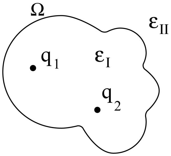
A mixed discrete-continuum model for biomolecule electrostatics. The surface Ω represents the dielectric boundary between regions with dielectric constants ∈I and ∈II. Partial atomic charges are located in region I, with illustrative charges q1 at r1 and q2 at r2. The Debye screening parameter κ is zero within region I and may be non-zero in region II. In work not described here, an ion-exclusion layer may also be treated [29, 30].
The Poisson problem in the interior and the linearized Poisson–Boltzmann problem in the exterior are coupled by continuity conditions at the boundary [31]. These coupled partial differential equations can be converted to integral equations in several ways. Problems in non-ionic solutions (those with κ = 0 in the solvent region) can be solved using the induced surface-charge method [32, 33]. When the ionic strength is non-zero, Green’s theorem can be applied to derive either a mixed first-second-kind integral formulation [34] or a purely second-kind formulation [35]. Chipman [36] has described and compared these and other formulations. We present the mixed formulation originally presented by Yoon and Lenho [34].
Applying Green’s theorem in both regions and applying the continuity conditions gives the coupled integral equations
| (1) |
| (2) |
Here, rΩ is a point on the surface; r’ is the integration variable on the surface; n(r’) is the normal at r’ pointing into solvent; ∫ denotes the principal value integral taken in the limit as a field point approaches r’ from the inside [31]; φ(r) and denote the potential and its normal derivative at the surface; qi is the ith of nc point charges; and GI(r; r’) and GII(r; r’) are the free-space Green’s functions for the governing equations in the two regions. Typically, , and , which is the free-space Green’s function for the linearized Poisson–Boltzmann equation.
To solve Eqs. 1 and 2 using a boundary-element method, the solute–solvent boundary is discretized and the surface variables are approximated as weighted sums of compactly supported basis functions, where the weights are selected so that the discretized integrals match a set of constraints (see, for example, references [37, 38]). In collocation methods, the residual is forced to be exactly zero at a set of points on the surface; in Galerkin methods, the residual is required to be orthogonal to the basis functions. Using collocation and piecewise constant basis functions such that the ith basis function is unity on the ith boundary element and zero elsewhere, we form a dense block matrix whose entries take the form
| (3) |
where ri denotes the collocation point associated with the ith boundary element and K(r; r’) is either a Green’s function or a Green’s function derivative with respect to the surface normal at r’.
2.1.2. Surface Generalized Born
The generalized Born (GB) model of solute–solvent electrostatic interactions yields a more easily computed approximation to energies derived by solving the Poisson–Boltzmann equation [5]. The GB pairwise energy Ui,j between charges i and j is given by
| (4) |
where qi and qj are the charge values and Ri and Rj are the Born radii. The Born radius Ri for an atom or group of the solute is defined such that a sphere with radius Ri and centrallylocated unit charge has solvation energy equal to that of the entire molecule if qi = 1 and qj = 0 ∀ ≠ i.
Still et al. proposed an approach to calculating the Born radius Ri by relating the volume integral
| (5) |
to the analytical expression for the solvation energy of a centrally located charge in a spherical dielectric cavity [5]. In this equation, Vint is the volume of the solute interior and r’ denotes the integration variable. Similar expressions to calculate Born radii have also been presented [7, 39, 40]. Ghosh et al. introduced the surface-generalized-Born (sGB) method [7], in which an application of the divergence theorem converts Eq. 5 to the surface integral
| (6) |
where S denotes the dielectric boundary. For our calculations, we used the Richards molecular surface described in Section 2.2.
2.1.3. Continuum van der Waals
Levy et al. described a continuum method to model the van der Waals interactions between solute and solvent, assuming a constant solvent density and using a spherical model for a water molecule [8]. In this model, the interaction energy is then expressed as an integral over the solvent volume,
| (7) |
where n denotes the number of atoms in the solute, ρw the bulk water number density, and the van der Waals potential between atom i and a water molecule located at a distance r = ∥r’ – ri∥ from the atom center ri.
Because the van der Waals potential is defined by the distance from a water molecule center to an atom center, the solvent-accessible surface [22] is the natural solute–solvent boundary definition for the integral in Eq. 7. If the van der Waals potential is modeled by the Lennard-Jones 6–12 function,
| (8) |
then the divergence theorem applied to the integral in Eq. 7 yields
| (9) |
2.2. Defining Molecule–Solvent Interfaces
Figure 2 illustrates the three most prevalent definitions for the solute–solvent boundary, using a two-atom example. A molecule’s van der Waals surface, as shown in Figure 2(a), is defined to be the boundary of a union of spheres. Each sphere represents an atom centered at a particular location in space and the sphere radius is set to the atom’s van der Waals radius; for reduced-atom models such as the polar-hydrogen CHARMM19 model [41], some spheres represent groups of atoms. The Lee and Richards solvent-accessible surface [22], depicted in Figure 2(b), is also a union of spheres; in this definition, each sphere’s radius is equal to the atom or group’s van der Waals radius plus the radius of a spherical probe molecule that is rolled over the union of atoms. Both the van der Waals and solvent-accessible surfaces can be constructed by forming a union of “patches,” where each patch is the intersection of a given atom’s sphere with a set of half-spaces [23].
FIG. 2.

Three definitions of solute–solvent boundaries, shown for a two-atom case: (a) van der Waals surface. (b) The Lee and Richards solvent-accessible surface. (c) The Richards Solvent-excluded (molecular) surface. The dotted lines in (b) and (c) denote the van der Waals surface.
Richards [28] defined the molecular surface, or solvent-excluded surface, and Connolly [23] presented an algorithm for its analytical determination. As illustrated in Figure 2(c), the molecular surface is defined by rolling a probe sphere over the union of atomic spheres with van der Waals radii; the surface consists of the set of points corresponding to the probe sphere’s closest approach to the boundary of the union. In this definition, the regions of the molecular surface that correspond to probe positions at which the probe contacts the sphere union at only one position are said to belong to the contact surface; such convex, spherical surface patches are called caps [23]. In contrast, the reentrant surface comprises regions that correspond to probe positions at which the probe touches the sphere union at multiple points. Where the probe touches two spheres of the union, its movement is restricted by one degree of freedom; a toroidal piece of surface, or belt, is then produced as the probe rotates about the axis defined by the two sphere centers. Where the probe touches the union at three or more points, a concave spherical surface patch is defined; this type of face is termed a pit. All three types of surface patches, or faces, are bounded by circular arcs, and molecular surfaces can be represented exactly as a finite union of different instances of these surface patches [23].
Many researchers have presented algorithms to discretize solvent-excluded and solvent-accessible surfaces [19, 42–50]. These algorithms take as input the atom centers and their radii, as well as the probe-sphere radius, and return a set of boundary elements that approximate the molecular or accessible surface. Surface approximation accuracy is usually improved by using more, but smaller, boundary elements. Most work has focused on generating planar-triangle-based surface discretizations, but several groups have developed more sophisticated approaches. Zauhar and Morgan have reported cubically-curved elements [33, 51], Juffer et al. used cubic interpolation [35], Bajaj et al. used B-spline patches [42], and Bordner and Huber used quadratically-curved elements [52]. Zauhar has presented an approach to exactly discretize a smooth approximation to the molecular surface such that the surface has a continuous normal [19]. Liang et al. find an exact solvent-accessible surface derived from alpha shapes but solve problems on an exactly-curved approximation to this surface [25, 45, 46]. Our approach exactly discretizes the Richards molecular surface using Connolly’s method, and we solve problems on this exact representation using numerical integration techniques specialized for these surfaces.
3. SURFACE DISCRETIZATION
As discussed in Section 2.2, three common solute–solvent boundary definitions can be represented as the union of portions of toruses and spheres, where the surface construction ensures that the boundaries between different surface patches are formed by arcs of circles. In this Section we define two classes of curved surface elements that permit the exact discretization of the solute–solvent boundaries.
3.1. Toroidal Element Definition
A torus is defined by revolving a circle about an axis that lies in the same plane as the circle; referring to Figure 3, z is the axis of revolution, and the dotted circle is being revolved about this axis. The circle center, normal, and revolution axis together define a local coordinate system, and it is useful to describe the torus as having an outer radius c, which is the shortest distance between the circle center and the revolution axis, and inner radius a, which is the radius of the circle. With z as the axis of revolution, we complete the coordinate system by defining y parallel with the normal of the circle at the revolution starting position, and the coordinate system origin so that the circle center lies in the x – y plane. Given such a coordinate system, two angular coordinates, θ and ψ, shown in Figure 3 suffice to specify any point on the torus. The angle θ describes how far the circle has revolved about z, and the angle ψ determines the point’s position on the circle at θ, and is defined such that ψ = 0 points radially outward from the coordinate system origin and ψ = π points radially inward. We define a torus element as the portion of a torus with angular coordinates θ1 ≤ θ ≤ θ2 and ψ1 ≤ ψ ≤ ψ2. Any toroidal surface patch on a solvent-excluded surface can be exactly discretized using such torus elements. One toroidal element is shown in Figure 3. The circle center, as it revolves around the axis of revolution z, traces a circle, which is shown in black in the Figure. We number and define the edges of the torus in a right-handed manner (i.e., the interior of the element is to the left as one traverses the edges). Because the toroidal surface patches form part of the reentrant surface, the torus element normal points into the finite volume enclosed by the torus.
FIG. 3.

Specification of a torus and a torus element with 0 ≤ θ ≤ π/3 and π/2 ≤ Ϙ ≤ 5π/6.
3.2. Spherical Element Definition
We define a generalized spherical triangle (GST) to be a three-sided region of a sphere’s surface whose edges are formed by three circular arcs [9]. The arcs are not permitted to intersect except at their endpoints, which are the vertices of the generalized spherical triangle. Furthermore, the local interior angles must be less than π radians. This definition contrasts with a regular spherical triangle, whose arcs are portions of great circles on the sphere. Figure 4 illustrates a GST in which one arc is a portion of a small circle and the others belong to great circles. The arcs are oriented and numbered in a right-handed fashion, following standard mathematical convention. Convex spherical patches have a normal pointing away from the sphere center. Concave spherical patches, which are formed only in solvent-excluded surfaces at points where the probe sphere touches three or more atoms simultaneously [28], have a normal pointing towards the probe-sphere center, because the concave patch must point out into the solvent region. Small-circle arcs are generally needed to resolve the boundaries between different surface patches [19]; if only great-circle arcs are used to form element boundaries, the elements intersect each other rather than meeting exactly at the boundaries. Curved-element discretizations of van der Waals and solvent-accessible surfaces can also be generated by taking a triangularized surface and projecting the planar triangle edges out to the appropriate sphere surfaces [25]; the surface elements so generated have exact curvature, but their edges are all arcs of great circles.
FIG. 4.

A generalized spherical triangle (GST) with one bounding edge belonging to the circle centered at the blue dot. The remaining edges belong to great circles on the sphere.
4. CURVED-ELEMENT INTEGRATION METHODS
In this section, numerical techniques are presented to evaluate integrals of the form
| (10) |
where Ω is either a toroidal or generalized spherical triangle element, as defined in Section 3. For the problems discussed in this work, the function K(r; r’) is singular at r = r’ and decays monotonically to zero as ∥r – r’∥ → ∞. For smooth integrands such as far-field integrals in which r is far from Ω, the integration may be performed using numerical quadrature. We present specialized methods for smooth integrands in Section 4.1. Integrals for which r ∈ Ω or is sufficiendtly close that the integrand varies extremely rapidly (near-field integrals), require special techniques, which we present in Section 4.2.
4.1. Far-Field Quadrature
When the evaluation point r in Eq. 10 is sufficiently far from the domain of integration Ω, K(r; r’) varies smoothly over Ω and therefore relatively low-order numerical quadrature provides accurate results. A qth-order quadrature rule estimates the integral of a function f over a simple domain Γ as a weighted sum of function evaluations at q specified points in Γ as
| (11) |
The values wi are quadrature weights for the quadrature points xi. Many types of quadrature rules are designed such that they give exact or nearly exact results if the domain is simple and the integrand is a sufficiently low-order polynomial. For simple integration domains like planar triangles, well-established rules such as those presented by Stroud [10] offer excellent accuracy.
To integrate a function over a more complex domain Ω, one typically determines a smooth coordinate transformation M from a simple domain Γ, which has a known quadrature rule, to the domain of integration Ω. Applying the chain rule transforms the integral of Eq. 10 to the form
| (12) |
where denotes the integration variable in Γ and is the determinant of the Jacobian of M at . A q-point quadrature rule for the domain Γ allows Eq. 10 to be approximated as
| (13) |
Because the original integrand over Ω is multiplied in the new integral by the Jacobian determinant ∣J∣, it is essential that the product of the original integrand and the coordinate transformation be smooth; that is, K∣J∣ should vary smoothly over Γ. Such coordinate transformations for the curved elements presented in the preceding subsection are described next.
4.1.1. Generalized Spherical Triangle Coordinate Transformation
Zauhar has presented one coordinate transformation between a planar triangle and what we have defined as the generalized spherical triangle (GST) [19]. We present an alternative. Figure 5 illustrates the coordinate transformation from a simple domain Γ, the standard planar triangle of Figure 5(a) with vertices {(0, 0)T; (1, 0)T; (0, 1)T}, to the more complicated GST domain Ω, shown in top and side views in Figures 5(b) and 5(c). The GST has been rotated so that the longest arc, labeled a1, lies in a plane perpendicular to the x-axis and the arc midpoint lies in the y = 0 plane. The standard triangle parametric coordinates (ξ,η)T are first mapped to the spherical coordinate system (θ,ψ)T, illustrated in Figures 5(b) and (c), and then trivially transformed to Cartesian coordinates. The angle ψ measures the angle from the positive x-axis and the angle θ measures rotation about the x-axis such that a point with θ = 0 lies in the y = 0 plane.
FIG. 5.

(a) The standard unit triangle in parametric coordinate space. (b) A GST viewed from the negative y-axis. The angle Ϙ is measured relative to the positive x-axis. Each Ϙ is mapped to one plane with normal along the x-axis; the plane intersects the sphere and defines a circle. (c) A GST viewed from the positive z-axis. Dashed lines indicate the circle of intersection between the sphere surface and the plane specified by φ. The angle θ specifies the rotation about the x-axis. The image of the standard-triangle vertices under the coordinate transformation are labeled.
The reference triangle edge from to is mapped to the GST edge from v3 to v1. Letting (θi,ψi)T denote the spherical coordinates of GST vertex vi, it is clear that ψ1 = ψ2. As shown in Figure 5, every line of constant η in the standard triangle is mapped to an arc of the circle defined by ψ = ψ1 + η(ψ3 – ψ1); restricting v3 to lie above the z = 0 plane ensures that every η defines a unique circle and that every circle intersects the v2 – v3 and v3 – v1 arcs exactly once. For a given η, the arc endpoints are defined by the intersection of the circle at elevation angle ψ with the arcs a2 and a3. A point (ξ,η)T in the reference triangle is mapped to this arc by mapping the point’s parametric distance to a parameterized form of the arc at ψ between a2 and a3. This mapping is guaranteed to exist if the vertex v3 is further from the plane of arc a1 than any other point on the arcs a2 and a3. The restrictions are imposed during surface discretization. Appendix B contains the full derivation of the coordinate transformation and its Jacobian.
4.1.2. Toroidal Element Coordinate Transformation
A torus element is isomorphic to a rectangle. A simple mapping suffices to transform the unit rectangle, with vertices {(0, 0)T; (0, 1)T; (1, 1)T; (1, 0)T}, to an arbitrary torus element defined by {(θ,ψ)∣θ ∈ [θ1,θ2],ψ ∈ [ψ1,ψ2]}. For the torus in Figure 3, with outer radius c, inner radius a, centered at the origin, and with axis of revolution along the z-axis, the Cartesian coordinates of a point at (ξ,η)T in parametric coordinates are
| (14) |
where θ = θ1 + ξ(θ2 – θ1) and ψ = ψ1 + η(ψ2 – ψ1). The determinant of the Jacobian is
| (15) |
4.2. Near-field Integration Techniques
The integrands of interest have singularities as the evaluation point approaches the domain of integration. As a result, even high-order Gaussian quadrature rules fail to accurately approximate the singular and near-singular integrals; more sophisticated techniques are required. In this section we present techniques for integrating the Laplace kernel K(r; r’) = 1/(4π∥r – r’∥) and its normal derivative . Appendix C describes how these methods may be adapted for the linearized Poisson–Boltzmann, surface-generalized-Born, and continuum-van der Waals kernels.
4.2.1. Single-Layer Potential
The integral
| (16) |
is referred to as the single-layer potential because it represents the potential induced by a unit-density monopole charge layer on the integration domain Ω. Accurate evaluation of such integrals is fundamental to the accuracy of the boundary-element methods as described here.
a. Spherical Element Single-Layer
When Ω is a generalized spherical triangle, the method of Wang et al. can be applied to evaluate the integral in Eq. 16 [9, 53]. In this method, the chain rule is used to replace the integral over the GST of a given charge distribution with an integral of a modified charge distribution f(r) over the planar domain Γ. The domain Γ is chosen such that the potential induced by the modified charge distribution f(r) can be accurately approximated using well-established techniques [13, 54]. For the applications discussed in this paper, Γ is chosen so that the reference domain Γ lies tangent to the GST at the GST centroid. Figure 6 illustrates the approach. For uniform distributions on the GST (that is, ), the relation
| (17) |
defines the reference-element monopole charge distribution f(r), which is the term in parentheses in the third integral that exactly reproduces the curved-element induced potential. In Eq. 17, is a point in the flat element, is its image under the coordinate transformation from Γ to Ω, and is the Jacobian of the mapping. Because the flat element is tangent at the centroid and the sphere has constant curvature, f(r) uniformly approaches ∣J∣ at the centroid, and the smoothness of f(r) allows it to be represented approximately using a low-order polynomial [53]. The integrals over Γ can then be computed as
| (18) |
where the polynomial coefficients are denoted by αi,j and each monomial integral on the right-hand side can be calculated using the methods of Newman or Wang [13, 54]. The coefficients {αi,j} are found by least-squares solution of the Vandermonde matrix equation
| (19) |
where denotes the ith of n sample points, and n must be greater than the number of coefficients to be fit.
FIG. 6.
Schematic of the approach for evaluating the potential induced by a distribution of monopole charge on a generalized spherical triangle. A planar reference element viewed edge-on (blue) is defined to be tangent to the original GST (black solid arc) at the GST centroid. The reference element vertices are defined to be the projection of the GST vertices to the plane tangent to the GST centroid.
The mapping from the flat reference element can be defined in one of two ways. In the first, the flat element edges are defined by casting rays from the sphere center through the GST boundary arcs to the tangent plane. Boundary arcs that are segments of great circles map to straight lines in this projective transformation, and any arc belonging to a small circle becomes a portion of a conic curve (either a hyperbola or an ellipse). The monomial integrals can then be evaluated by analytical integration over a triangular domain, followed by addition or subtraction, as necessary, of the result of numerical quadrature over the conic region [9]. An alternative method is to project the GST vertices to the tangent plane, which defines a triangle. The mapping between this reference triangle and the GST is then a composition of two mappings: the first transforms the reference triangle to the standard triangle, and the second transforms the standard triangle to the GST. The first mapping is straightforward, and methods for the second mapping have been presented in Section 4.1.1.
We emphasize that our selection of a flat reference element that lies tangent at the GST centroid suffices for the kernels specified in this work and for BEM approaches based on piecewise-constant basis functions and centroid-collocation; other problems may require that a reference element be defined in relation to the evaluation point [53].
b. Toroidal Element Single-Layer
When Ω is a toroidal element, the previously-described polynomial-fitting method is difficult to apply because the torus surface has unequal radii of curvature at most points. As a result, the ratio takes different limits depending on the direction from which r’ approaches r, and this phenomenon necessitates the development of more complicated coordinate transformations. Instead, recursive subdivision is applied to evaluate near-field integrals [55].
The element integral is evaluated in one of two ways. We denote the element centroid by rc and its area by A. If the evaluation point r satisfies the element is split into four sub-elements defined by equally dividing the angular ranges. The subelement integrations are then evaluated independently. Further subdivision may be required, depending on the position of the evaluation point relative to the four new centroids and the new element areas. The second near-field integration method is applied when the evaluation point lies at the element centroid (i.e., r = rc). This case arises for boundary-elementmethod problems solved using centroid-collocation schemes. Symmetry in the θ direction allows these integrals to be evaluated for half the computational expense of a full subdivision. For the molecular applications described here, both subdivision integration methods halt the subdivision when the divided elements have no edges longer than 10−5 Å.
4.2.2. Double-Layer Potential
The double-layer integral
| (20) |
represents the potential due to a unit-density dipole charge layer on the domain. The Wang et al. approach for double-layer integrals cannot be used for singular integrals. The ratio is not defined on the reference element because vanishes for all r’ ≠ r in the plane of the dipole layer.
We instead use the double-layer calculation presented by Willis et al. [56], which extends the work of Newman [13]. Recall that the potential induced by a normally-oriented dipole charge layer of uniform density equals the solid angle subtended by the integration domain at the evaluation point r [31]. Exploiting this characteristic, Newman derived an analytic expression for the double-layer potential induced by a uniform dipole distribution on a boundary element bounded by straight line segments [13]. Willis et al. extended Newman’s work to uniform distributions on curved elements, noting that the subtended solid angle can be found using quadrature [56].
Figure 7 illustrates this approach for evaluating the double-layer potential in Eq. 20. The evaluation point r is translated to the origin and the coordinate system is rotated so that the element centroid lies on the z-axis. We define a sphere of unit radius centered at the origin and cast rays from the origin through the element edges to the sphere surface. The projected edges define a region on the sphere, and we find the desired solid angle by simply computing the bounded area:
| (21) |
Separating the integration into a sum of integrals over each of the ne circular arcs that form the element boundary, and changing variables from θ to a parametric t along the arcs, we have
| (22) |
where t is the parametric coordinate along the ith edge, and θi(t) is the azimuthal angle of the point at position t along the ith arc. Note that the element edges can be projected to the sphere regardless of how the edges are positioned relative to the unit sphere onto which they are projected. Figures 8(a) and 8(b) are illustrations of this fact.
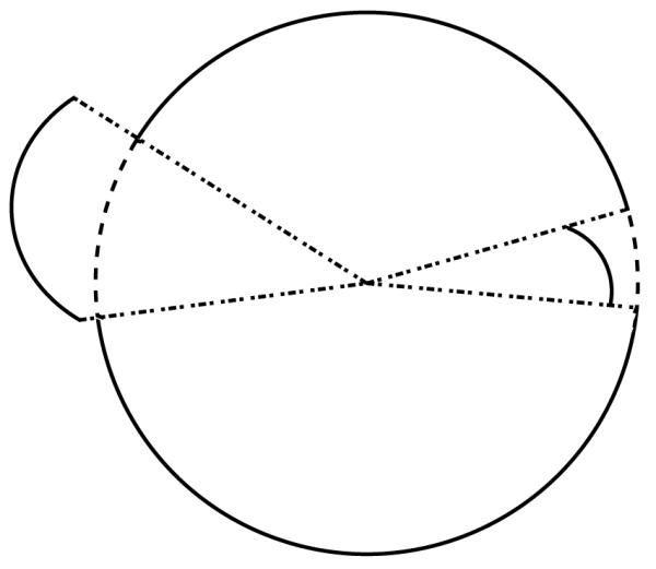
FIG. 7.

The Newman approach to calculating the potential induced by a uniform distribution of a normally-oriented dipole charge layer [13]. The cross at the center of the sphere denotes the point at which the potential is to be determined; the thin arcs form the edges of a GST; the thick lines represent the projection of the GST bounding arcs to the sphere. The double-layer potential, which equals the solid angle bounded by the thick lines, is directly proportional to the bounded area.
FIG. 8.
Edges may be projected to the unit sphere regardless of their position relative to it.
The directional character of the double-layer potential deserves comment. The integral of Eq. 20 is discontinuous as the evaluation point r approaches and passes through the surface. The value of the integral is defined to be the limit as r approaches the surface; when r ∈ Ω, therefore, the side from which r approaches the surface will determine the value of the integral. The two limits sum to 4π [31]. By convention, we assume that the integral has been taken as the evaluation point approaches from the side opposite of the normal direction.
An alternate approach, applicable only to uniform distributions, can also be taken. According to the Gauss–Bonnet theorem [57], the area bounded by the projected arcs can be determined following integration of the geodesic curvature of the projected edges. Finally, we note that the Willis et al. approach is applicable not only to spherical and toroidal surface elements but also to many other types of curved surface elements [56].
5. RESULTS
We have generated several curved-element discretizations using the process outlined in Appendix A and implemented the numerical integration methods in both C and MAT-LAB [58]. Flat-triangular surface discretizations have been produced using Connolly’s Molecular Surface Package (MSP) [59]. We first present results that validate the surface discretizations and the integration techniques; we then demonstrate the advantages of curved-element surface methods with several representative calculations on small molecules. Far-field numerical integrations have been performed using the 16-point quadrature rule presented in Stroud [10], and the GST single-layer integrals have been approximated by fitting to a 4th-order polynomial.
5.1. Problem Geometries
5.1.1. Alanine Tripeptide
The CHARMM molecular mechanics computer program [41] with the CHARMM22 parameter set [60] was used to generate two conformations of blocked alanine tripeptide (two alanine residues with an acetylated N-terminus and N-methylamide at the C-terminus). One conformation takes average ϕ and ϕ angles for a parallel β-sheet (ϕ = −119°, Ϙ= +113°); the other conformation takes the average angles for a right-handed α-helix (ϕ = −57°, Ϙ = −47°) [61].
5.1.2. Alanine Dipeptide
Scarsdale et al· has presented energy-minimized atomic coordinates for several conformations of the alanine dipeptide [62], which is a single alanine residue blocked as above. A set of curved-element surface discretizations at varying refinement was generated using these coordinates, PARSE radii [63], and a probe radius of 1.4 Å.
5.1.3. Barnase–Barstar Complex
The barnase–barstar complex of two proteins was chosen to serve as a larger test case to demonstrate the correctness of the surface discretization method and of the numerical integration methods. Coordinates were taken from reference 64 using accession number 1BRS in the Protein Data Bank [65].
5.2. Validating the Surface Discretization
The surface area of planar triangles as well as GST and toroidal elements can be calculated analytically. Therefore, the correctness of the presented curved-element discretization approach may be demonstrated without involving numerical integration.
The Gauss–Bonnet theorem [57] was used to analytically calculate the surface area of GST elements, following Connolly [23]. The theorem, when applied to a compact manifold, relates the integral of the curvature over the surface to the integral of the geodesic curvature of the boundary and the corner angles. A generalized spherical triangle has constant curvature over its surface, and its bounding arcs have constant geodesic curvature; accordingly, its area may be calculated analytically. For a toroidal element defined according to Section 3.1, the analytical area is
| (23) |
We generated both flat-element and curved-element surface discretizations of several molecules at varying levels of refinement, using the Richards molecular surface definition [28] and the solvent-accessible surface. PARSE radii [63] and a 1.4 Å probe radius were used for molecular surface generation and CHARMM22 radii [60] were used for solvent-accessible surfaces. The analytical areas calculated by Connolly’s program MSP [59] were used as a reference for the calculated analytical areas of the planar-element and curved-element discretizations. Tables I and II present the molecular-surface and solvent-accessible-surface results. These calculations, which incur no numerical approximation, illustrate that even coarse curved-element discretizations accurately capture the surface geometry. Similar results (not shown) have been obtained for van der Waals surfaces, which like the solvent-accessible surfaces have spherical but not toroidal elements. It is especially noteworthy that planar-element discretizations with significantly more elements than their curved-element counterparts were not yet converged to the correct surface area. The exact geometric description inherent to the presented curved-element methods could lead to significantly more accurate numerical calculations than those based on approximate-geometry planar-element discretizations.
TABLE I.
Comparison of discretized surface areas with analytical molecular (solvent-excluded) surface area. Probe radius is taken to be 1.4 Å. All area quantities are in Å2 and have been rounded to the nearest 0.001 Å2.
| METHOD | |||||
|---|---|---|---|---|---|
| PROBLEM | ANALYTICAL AREA | AREA OF DISCRETIZED SURFACE | |||
| FLAT | CURVED | ||||
| # ELEMENTS | AREA | # ELEMENTS | AREA | ||
| Atom | |||||
| COARSEa | 74 | 11.516 | 40 | 12.566 | |
| MEDIUMb | 12.566 | 270 | 12.249 | 70 | 12.566 |
| FINEc | 448 | 12.390 | 124 | 12.566 | |
| Parallel-β alanine tripeptided | |||||
| COARSEa | 684 | 230.965 | 1326 | 241.642 | |
| MEDIUMb | 241.642 | 1944 | 238.450 | 1781 | 241.642 |
| FINEc | 2904 | 239.617 | 2923 | 241.642 | |
| Barnase–barstar complexe | |||||
| COARSEa | 29728 | 7979.774 | 63915 | 8269.077 | |
| MEDIUMb | 8269.077 | 79104 | 8188.538 | 88860 | 8269.077 |
| FINEc | 149160 | 8407.962 | 133676 | 8269.077 | |
MSP angle = 1.0, NETGEN level = VERY COARSE
MSP angle = 0.5, NETGEN level = COARSE
MSP angle = 0.4, NETGEN level = MEDIUM
Structure preparation is described in Section 5.1.1
From reference 64, entry 1BRS in the Protein Databank [65].
TABLE II.
Comparison of discretized surface areas with analytical solvent-accessible surface area. Probe radius is taken to be 1.4Å. All area quantities are in Å2 and have been rounded to the nearest 0.001 Å2.
| METHOD | |||||
|---|---|---|---|---|---|
| PROBLEM | ANALYTICAL AREA | AREA OF DISCRETIZED SURFACE | |||
| FLAT | CURVED | ||||
| # ELEMENTS | AREA | # ELEMENTS | AREA | ||
| Atom | |||||
| COARSEa | 74 | 66.334 | 40 | 72.382 | |
| MEDIUMb | 72.382 | 270 | 70.554 | 68 | 72.382 |
| FINEc | 448 | 71.368 | 124 | 72.382 | |
| Parallel-β alanine tripeptided | |||||
| COARSEa | 396 | 437.304 | 564 | 467.815 | |
| MEDIUMb | 467.815 | 1268 | 459.406 | 714 | 467.815 |
| FINEc | 1846 | 462.617 | 1064 | 467.815 | |
| Barnase–barstar complexe | |||||
| COARSEa | 10643 | 8785.722 | 20053 | 9152.150 | |
| MEDIUMb | 9152.150 | 31800 | 9094.782 | 25835 | 9152.150 |
| FINEc | 87178 | 9571.220 | 38767 | 9152.150 | |
MSP angle = 1.0, NETGEN level = VERY COARSE
MSP angle = 0.5, NETGEN level = COARSE
MSP angle = 0.4, NETGEN level = MEDIUM
Structure preparation is described in Section 5.1.1
From reference 64, entry 1BRS in the Protein Databank [65].
5.3. Validating Curved Boundary-Element Integration
After verifying that the curved-element discretizations accurately describe the desired surfaces, the numerical integration methods presented in Section 4 must also be validated. Surface-area calculations, which entail the evaluation of integrals like Eq. 10 with the simplest integrand K(r; r’) = 1, offer an excellent opportunity for this validation. One can verify the correctness of the discussed coordinate transformations by computing surface areas using the presented numerical quadrature techniques; as can be seen from Eq. 12, the surface area of an element is calculated as the integral of the Jacobian determinant over the reference element. Because the determinants vary smoothly over the reference domains, these integrals should be evaluated with high accuracy; however, because the Jacobian determinants are not actually low-order polynomials, the numerical results are not expected to exactly match analytical results. Table III lists the pit, belt, and cap areas calculated by analytical and direct quadrature methods, and also by the polynomial-fitting method for the pit and cap surfaces. The numerical and analytical results agree extremely well for coarse discretizations. The smaller elements present in finer discretizations exhibit less deviation from planarity; consequently, the Jacobians are smoother and finer discretizations offer higher accuracy area calculations when using polynomial fitting. The polynomial-fitting method calculations, which are important for evaluating singular and near-singular integrals rather than for smooth integrands, are included to demonstrate the accuracy of the fitting procedure.
TABLE III.
Comparison of pit, belt, and cap areas computed by analytical, direct quadrature, and polynomial-fitting metho ds, using the molecular surface discretizations of Section 5.2. All area quan tities are in Å2 and have been rounded to the nearest 0.001 Å2.
| METHOD | |||||||
|---|---|---|---|---|---|---|---|
| COARSE | MEDIUM | FINE | |||||
| PROBLEM | ANALYTICAL | DIRECT | FIT | DIRECT | FIT | DIRECT | FIT |
| Atom | |||||||
| CAP | 12.566 | 12.566 | 12.567 | 12.566 | 12.566 | 12.566 | 12.566 |
| Parallel-β blocked alanine trip eptide | |||||||
| PIT | 18.719 | 18.719 | 18.720 | 18.719 | 18.719 | 18.719 | 18.719 |
| BELT | 77.565 | 77.565 | – | 77.565 | – | 77.565 | – |
| CAP | 145.358 | 145.358 | 145.340 | 145.358 | 145.354 | 145.358 | 145.358 |
| Barnase–barstar complex | |||||||
| PIT | 2453.293 | 2453.240 | 2453.390 | 2453.292 | 2453.300 | 2453.293 | 2453.291 |
| BELT | 3195.626 | 3195.626 | – | 3195.626 | – | 3195.626 | – |
| CAP | 2620.158 | 2620.130 | 2619.698 | 2620.154 | 2620.056 | 2620.157 | 2620.137 |
5.4. Surface-Generalized-Born Calculations
The surface discretization and integration techniques presented in this work have been used to calculate Born radii using the surface-generalized-Born method introduced by Ghosh et al. [7] and surface formulations of the Grycuk [39] and Wojciechowski and Lesyng [40] Generalized Born models. The surface integrals associated with these calculations are never singular because every evaluation point is the center of a sphere. Figure 9 is a plot of the Born radii computed for the alanine tripeptide in α-helical and parallel-β conformations using a surface formulation of the Grycuk method; results are shown for several levels of surface discretization. Shown for comparison are the Born radii calculated by volume integration using a fine cubic grid. Note that the surface-generalized-Born radii do not appreciably change as the discretization is refined. Similar results are obtained using the method of Ghosh et al· and that presented by Wojciechowski and Lesyng (data not shown). The insensitivity of the calculated radii, and therefore energies, with respect to surface discretization, illustrate one of the important advantages of curved-element methods: excellent numerical accuracy can be obtained with relatively few degrees of freedom, provided that an accurate representation of the surface geometry is used.
FIG. 9.

Generalized Born radii calculated by volume integration and by evaluating surface integrals based on the GB model proposed by Grycuk [39]. The volume radii are plotted as large squares and the surface GB radii are plotted with circles, triangles, crosses, and diamonds. (a) Alpha-helix blocked alanine tripeptide. (b) Beta-sheet blocked alanine tripeptide.
5.5. Continuum van der Waals Calculations
The surface-continuum van der Waals formulation has been implemented [9] and tested for four of the alanine dipeptide conformations presented by Scarsdale et al. [62]. Solvent-accessible surfaces were defined using OPLS all-atom radii [66] and a probe radius of 0.85 Å, in accordance with the Levy et al. parameterization [8] for the TIP4P water model [67]. The Lennard-Jones coefficients for each surface integral of the form in Eq. 9 were determined by appropriately mixing the well depths ∈ and the diameters σ for each OPLS atom type and the TIP4P water model. In Table IV are listed the energies computed using a volume method as well as curved-element and planar-element surface methods. Volume integrals were evaluated numerically, one atom at a time, using a spherical grid. These results illustrate that high accuracy is achievable with coarse discretizations provided that the discretizations accurately represent the problem under study.
TABLE IV.
Solute–solvent van der Waals interaction energies estimated using a volume integration scheme and using a surface formulation of the Levy et al. continuum van der Waals model [8] and curved surface elements. All energies are in kcal/mol and have been rounded to the nearest 10−4 kcal/mol.
| c5 | αR | c7eq | c7ax | |||||
|---|---|---|---|---|---|---|---|---|
| Volume | −10.1365 | −9.8917 | −10.0190 | −9.9199 | ||||
| # Elements | Energy | # Elements | Energy | # Elements | Energy | # Elements | Energy | |
|
|
||||||||
| Surface | 429 | −10.1369 | 486 | −9.8918 | 357 | −10.0193 | 421 | −9.9201 |
| 558 | −10.1366 | 611 | −9.8918 | 479 | −10.0192 | 541 | −9.9200 | |
| 901 | −10.1365 | 1033 | −9.8917 | 793 | −10.0191 | 863 | −9.9199 | |
| 1912 | −10.1365 | 2069 | −9.8917 | 1746 | −10.0190 | 1782 | −9.9199 | |
| 4877 | −10.1365 | 5247 | −9.8917 | 4245 | −10.0190 | 4585 | −9.9199 | |
| 10035 | −10.1365 | 10829 | −9.8917 | 10418 | −10.0190 | 10755 | −9.9199 | |
5.6. Poisson–Boltzmann Electrostatics Problems
The electrostatic component of the solvation energy for several small boundary-element systems has been computed using the Yoon and Lenho integral formulation (Eqns. 1 and 2) and dense preconditioned GMRES [68]. Larger systems must be solved using fast, kernel-independent BEM algorithms such as the fast multipole method or FFTSVD [69–71]. As described in Section 2.1.1, we have used piecewise-constant basis functions and centroid collocation. For all calculations, we assume that the solute region has ∈I = 4 and the solvent region has ∈II = 80.
5.6.1. Spherical Geometry
The solvation energy of a centrally-located charge in a spherical low-dielectric cavity can be computed analytically if the Laplace equation holds in the solvent region, or numerically using spherical harmonics if the linearized Poisson–Boltzmann equation holds in the solvent region. Figure 10 illustrates the improved accuracy of curved-element BEM relative to planar-element methods; Figure 10(a) plots convergence for non-ionic solutions (i.e., κ = 0 Å −1) and Figure 10(b) plots convergence to the analytical result when κ = 0.124 Å −1.
FIG. 10.

Convergence of solvation free energies for a centrally located charge in a 1 Å sphere, calculated by BEM numerical solution of the Yoon and Lenho integral equations. For both cases ∈I = 4 and ∈II = 80. (a) κ = 0 Å−1. (b) κ = 0.124 Å−1.
5.6.2. Alanine Dipeptide
Comparison of the alanine-dipeptide planar-element and curved-element energies to their values at the finest discretizations and plots of the absolute deviation as a function of the number of elements are shown in Figure 11.
FIG. 11.

Solvation free energies for four conformers of the alanine dipeptide; atom centers are those presented in [62] and PARSE atomic radii and partial charges have been used [63]. (a) c5 geometry. (b) αR geometry. (c) c7ax geometry. (d) c7eq geometry.
These electrostatics simulations on small molecules demonstrate that boundary-element method problems benefit significantly in accuracy given the correct representation of the dielectric interface. The ability of curved-element methods to reduce the needed basis set size to reach a target level of accuracy suggests that surface representation error, not basis set error, dominates modeling error.
5.7. PERFORMANCE
Analytic methods exist to compute the single- and double-layer potentials induced by a uniform or polynomially varying charge distribution on a planar element with straight edges [12, 13]. These methods are extremely efficient: potential computations involving a uniform charge distribution require only a single square root, natural logarithm, and inverse tangent operation per edge, whereas an N-point quadrature routine requires the calculation of N square roots. Curved-element methods are significantly slower. Table V lists the approximate number of panel integrals that can be computed per second on a 3.0 GHz Pentium IV processor using an implementation in C and the Intel C compiler with full optimizations.
TABLE V.
Approximate number of panel integrals per second computable using a C implementation of the presented techniques. All planar-triangle integrals have been computed by the methods of Hess and Smith [12] or Newman [13]. All far-field curved-element integrals have been computed using a 16-point quadrature rule. Self-term and near-field GST integrals have been computed using the polynomial-fitting scheme. Self-term and near-field toroidal-element integrals have been computed by recursive subdivision. A single-layer integral has been defined to be in the far field if the separation between the evaluation (field) point and the curved element exceeds four times the length of the element’s longest edge; a double-layer integral is defined to be in the far field if the separation exceeds twice the length of the longest edge.
| Single Layer | Double Layer | |||||
|---|---|---|---|---|---|---|
|
| ||||||
| Planar Triangle | GST | Toroidal Element | Planar Triangle | GST | Toroidal Element | |
| Self Term | 1,570,000 | 21,400 | 70 | 1,510,000 | 3,400 | 2,400 |
| Near Field | 1,570,000 | 20,700 | 5,100 | 1,630,000 | 25,800 | 18,600 |
| Far Field | 1,570,000 | 860,000 | 900,000 | 1,570,000 | 440,000 | 460,000 |
6. DISCUSSION
We have defined two classes of compact, curved, two-dimensional surface elements that can be used to exactly describe arbitrary solute–solvent boundaries according to the most commonly used boundary definitions. These curved-element surface discretizations can be used in a number of surface formulations of biophysical modeling problems. To numerically evaluate the desired surface integrals over these domains, we have described a set of accurate, efficient techniques specialized for these domains. Computational results illustrate the advantages of curved-element surface discretizations relative to those based on planar triangles.
One significant advantage of the curved-element representations is that the geometry of the discretized surface does not change as the discretization is refined. In contrast, flat-element discretizations describe different boundaries at differing refinements, as do curved-element discretizations based on quadratic or cubic shapes. Curved-element methods based on our discretizations, however, are limited only by the accuracy of the integration method used, and, for boundary-element method problems, also by the order of the basis functions. The curved-element method presented here therefore offers an attractive approach for calculating Born radii via the sGB method and for computing solute–solvent van der Waals interactions using a continuum model. Furthermore, curved-element quadrature in the far-field is as efficient as far-field flat-element quadrature, because one can use quadrature rules of the same order for both. As a result, problems that require the evaluation of many more far-field than near-field integrals can benefit significantly from curved-element methods without undue increase in computational expense. Finally, as a practical matter, the integration techniques presented in this work are straightforward to implement. A MAT-LAB [58] implementation, as well as planar- and curved-element discretizations of several small molecules, are available online [72].
Although the near-field integration techniques for curved elements are significantly slower than those required for flat elements [12, 13], the extra accuracy a orded may be invaluable for problems that require highly accurate solutions. Because curved elements allow a significant reduction in the number of unknowns, such discretizations provide a promising approach to reach a target level of accuracy given constraints on computer memory. Application to protein studies are being pursued [30]. These techniques can be extended to allow the evaluation of more complicated integrals, such as the potential induced by a polynomially-varying charge distribution on a curved element. Also, the curved-element discretization procedure may be modified to allow the production of coarser meshes.
ACKNOWLEDGMENTS
The authors are indebted to J.-H. Lee for useful discussions and to X. Wang for sharing his monomial integration software. This work was supported by the National Institutes of Health (GM065418 and CA096504), the Singapore–MIT Alliance, and the National Science Foundation. J. Bardhan gratefully acknowledges the support of a Department of Energy Computational Science Graduate Fellowship, and S. M. Lippow gratefully acknowledges the support of a National Science Foundation Graduate Fellowship. D. J. Willis gratefully acknowledges support from the Natural Sciences and Engineering Reseach Council of Canada.
APPENDIX A. EXTRACTING CURVED PANEL DISCRETIZATIONS
Accessible and van der Waals Surfaces
Accessible and van der Waals surfaces can be described by a set of spherical patches, where each patch represents a solvent-exposed portion of an atom. When an atom (or a probe-radius-expanded atom) intersects another, the two sphere surfaces form a circle of intersection, and all the atom’s surface beyond the plane of this circle is buried inside the other atom. Consequently, each spherical patch can be described by an intersection of the sphere and a set of half-spaces, which are derived by analytically solving for the planes of intersection between the given sphere and all the intersecting spheres. To mesh a spherical patch, we first obtain a high-quality flat triangular discretization using the program NETGEN [73]. NETGEN meshes surfaces based on a constructive solid geometry (CSG) scheme in which geometries are defined using boolean operations on primitives such as spheres and half-spaces.
Once the discretization is obtained, each planar triangle is converted to a GST by assigning an arc center to each edge. If an edge lies on one of the half-space planes, its arc center is assigned to be the center of the circle of intersection that defines the half-space. Occasionally, coarse triangular discretizations contain triangles whose edges lie on more than one plane. These situations do not reflect the molecular geometry but instead are a consequence of the NETGEN discretization procedure; such geometries are therefore discretized more finely. If a planar-triangle edge does not lie in a half-space plane, the arc center is assigned to be the center of the sphere; as a result, the corresponding GST arc is part of a great circle. After forming the GST, it is checked to ensure that it conforms to the definition presented in Section 3.2. Specifically, it is ensured that the arcs only intersect at their end points and that the internal jump angles are less than π radians. If any GST fails these checks, the entire spherical patch is rediscretized at a finer level.
Molecular Surfaces
Molecular surfaces are discretized in two stages. In the first stage, we increase the atomic radii by the probe radius and use NETGEN to generate a solvent-accessible surface by meshing the union of the expanded spheres. During the discretization process, NETGEN determines every point on the accessible surface where three or more expanded atoms simultaneously intersect, as well as every circular arc generated by the intersection of two expanded sphere surfaces. The intersection of three or more arcs becomes a fixed probe position for the molecular surface. The probe position generates one or more concave-spherical patches of reentrant surface because this point is simultaneously a probe-radius distance away from three or more atoms. Each circular arc connects two fixed probe positions along the intersection of two expanded atoms. Because the arc is composed of points equidistant from exactly two atoms, this arc indicates the presence of a toroidal surface patch. The accurate determination of these features is valuable during the second stage of discretization, in which the specified spherical and toroidal patches are meshed directly.
Spherical Contact Patches
Spherical contact patches on molecular surfaces are generated for every solvent-exposed atom. The patches are meshed similarly to the spherical patches on van der Waals and accessible surfaces; however, contact patches on molecular surfaces are bounded by the half-space planes located at sphere–torus intersections rather than at sphere–sphere intersections. The positions of these shifted planes are computed analytically by determining the point of tangency between the given sphere and the probe sphere when it simultaneously touches each neighboring atom.
Spherical Reentrant Patches
Spherical reentrant patches are meshed by placing a sphere of radius equal to the probe radius at each triple or higher intersection point determined during the discretization of the solvent-accessible surface. Recall that these intersection points are formed where multiple circular arcs meet, and that these arcs represent toroidal patches. The spherical reentrant patch is therefore intersected with three or more half-space planes, each of which represents a boundary between the probe sphere and the toroidal patch extracted from the corresponding circular arc.
Each plane is analytically defined by three points: the center of the probe sphere and the centers of the two atoms associated with the torus. When necessary, additional half-space planes are generated from probe-probe intersections in a manner similar to accessible surface meshing. Once the probe sphere and half-spaces have been identified, discretization proceeds identically to accessible spherical patch meshing.
Toroidal Patches
Each circular arc of the accessible surface is associated with one toroidal patch on the molecular surface. The arc traces out the path taken by the center of the sphere as it rolls tangent to its two associated atoms. Therefore, the toroidal patch is a portion of a torus centered at the analytical center of the circle of intersection between the two expanded atoms of the accessible surface. The torus’s principal x- and y-axes lie in the circle plane and the z-axis is parallel to the vector pointing between the atom centers. The torus’s inner radius a is the probe radius, and the outer radius c is the radius of the intersection circle.
If two probe positions terminate the accessible-surface arc, the toroidal patch will be bounded in θ. The range in θ is determined by fixing one torus principal axis to point from the torus center to the first probe position and then by taking the dot product of this axis with the vector pointing from the torus center to the second probe position. If the accessible-surface arc is not terminated by probe positions, the torus is complete, and spans [0, 2π] in the θ direction.
The bounds on are ψ found by the following procedure. First, specify an arbitrary probe position on the accessible-surface circle of intersection. Then, compute the vector pointing from the probe center to the center of the torus. Take the dot product of this vector with one pointing from the probe position to the center of each of the torus’s associated atoms. Each dot product is the cosine of one of the bounding angles ψ.
If the torus has an outer radius less than its inner radius (i.e., c < a), and if in addition the range in ψ overlaps the range , then the toroidal patch consists of two disconnected pieces of surface. The two regions of such a self-intersecting torus are meshed separately.
Once the bounds on the toroidal patch are determined, the region is discretized into toroidal panels by dividing the ranges of θ and into ψ an integral number of pieces such that the arc lengths of the panel edges are similar to those generated for GST panels.
APPENDIX B. COORDINATE TRANSFORMATION FROM THE STANDARD TRIANGLE TO THE GENERALIZED SPHERICAL TRIANGLE
In this appendix we describe how the parametric coordinates (ξ,η) map to a point (x, y, z) on a GST, and how we compute ∣J∣, the determinant of the transformation Jacobian. Figure 5 illustrates the spherical coordinate system; the coordinate ψ ∈ [0, π] describes the angle from the positive x-axis, and the coordinate θ ∈ [0, 2π] describes the angle from the positive z-axis. The angles ψstart and ψend are defined as shown in the Figure. For any point (ξ,η) we define a circle C(η) as shown; this circle is the set of points on the sphere at
| (24) |
Obviously . The intersection of C(η) with the two arcs a2 and a3 produce two points r2 and r3, which are defined to be at (θstart(η),ψ(η)) and (θend(η),ψ(η)). The θ coordinate of the mapped point is set to
| (25) |
We have also the first derivatives
| (26) |
| (27) |
Denoting the mapped point by , the Jacobian determinant is
| (28) |
where
| (29) |
| (30) |
Trivially, we have
| (31) |
| (32) |
| (33) |
The derivative is more challenging to calculate. The rotation angle θstart, defined by the relation
| (34) |
has the first derivative
| (35) |
where we have omitted adding the subscript start to the variables y and z, and the angle θend is defined analogously.
The derivatives and are defined by finding the angle α such that r satisfies
| (36) |
where rcenter is the center of the circle defining the GST arc and x and y form an orthonormal basis for the plane in which the arc lies. We then find the needed derivatives by
| (37) |
| (38) |
| (39) |
and taking the y and z components of .
APPENDIX C. CURVED PANEL INTEGRATION TECHNIQUES FOR OTHER INTEGRANDS
Linearized Poisson–Boltzmann Kernel
The single-layer linearized Poisson–Boltzmann integrals
| (40) |
can be evaluated by decomposing the integral into a sum of two easily computed integrals [70],
| (41) |
The first term is merely the single-layer Laplace integral, whose calculation we have already discussed. The second term is very smooth in the near-field when the elements are small compared to , and can therefore be integrated using the quadrature schemes described in Section 5.2. In the far-field, the entire integral in Eq. 40 can be computed easily using direct quadrature.
Double-layer linearized Poisson–Boltzmann integrals can be computed in an exactly analoguous fashion.
Surface-Generalized-Born Kernels
The surface-generalized-Born integrals all take the form of Eq. 6 but with different exponents depending on whether one begins from the volume formulations of Still et al., Grycuk, or Wojciechowski and Lesyng [5, 39, 40]. The required curved-element integrals are all nonsingular because the evaluation points are always sphere centers. The integrands’ rapid decay allows far-field quadrature to be used to compute all needed interactions.
Continuum van der Waals Kernels
The surface continuum van der Waals method requires evaluation of surface integrals of the form shown in Eq. 9, where again the evaluation points are always sphere centers. The scvdW integrals over the solvent-accessible surface are therefore never singular, and again far-field quadrature techniques may be used.
References
- [1].Tanford C, Kirkwood JG. Theory of protein titration curves I. General equations for impenetrable spheres. J. Am. Chem. Soc. 1957;59:5333–5339. [Google Scholar]
- [2].Warwicker J, Watson HC. Calculation of the electric potential in the active site cleft due to alpha-helix dipoles. J. Mol. Biol. 1982;157:671–679. doi: 10.1016/0022-2836(82)90505-8. [DOI] [PubMed] [Google Scholar]
- [3].Sharp KA, Honig B. Electrostatic interactions in macromolecules: Theory and applications. Annu. Rev. Biophys. Bio. 1990;19:301–332. doi: 10.1146/annurev.bb.19.060190.001505. [DOI] [PubMed] [Google Scholar]
- [4].Davis ME, McCammon JA. Electrostatics in biomolecular structure and dynamics. Chem. Rev. 1990;90:509–521. [Google Scholar]
- [5].Still WC, Tempczyk A, Hawley RC, Hendrickson TF. Semianalytical treatment of solvation for molecular mechanics and dynamics. J. Am. Chem. Soc. 1990;112(16):6127–6129. [Google Scholar]
- [6].Qiu D, Shenkin PS, Hollinger FP, Still WC. The GB/SA continuum model for solvation. A fast analytical method for the calculation of approximate Born radii. J. Phys. Chem. A. 1997;101(16):3005–3014. [Google Scholar]
- [7].Ghosh A, Rapp CS, Friesner RA. Generalized Born model based on a surface integral formulation. J. Phys. Chem. B. 1998;102:10983–10990. [Google Scholar]
- [8].Levy RM, Zhang LY, Gallicchio E, Felts AK. On the nonpolar hydration free energy of proteins: Surface area and continuum solvent models for the solute–solvent interaction energy. J. Am. Chem. Soc. 2003;125:9523–9530. doi: 10.1021/ja029833a. [DOI] [PubMed] [Google Scholar]
- [9].Bardhan JP, Altman MD, Lippow SM, Tidor B, White JK. A curved panel integration technique for molecular surfaces. Modeling and Simulation of Microsystems (Nanotech) 2005;volume 1:512–515. [Google Scholar]
- [10].Stroud A. Approximate Calculation of Multiple Integrals. Prentice Hall; 1971. [Google Scholar]
- [11].Ruehli AE, Brennan PA. Efficient capacitance calculations for three-dimensional multiconductor systems. IEEE T. Microw. Theory. 1973;21:76–82. [Google Scholar]
- [12].Hess JL, Smith AMO. Calculation of non-lifting potential flow about arbitrary three-dimensional bodies. J. Ship Res. 1962;8(2):22–44. [Google Scholar]
- [13].Newman JN. Distribution of sources and normal dipoles over a quadrilateral panel. J. Eng. Math. 1986;20(2):113–126. [Google Scholar]
- [14].Nedelec J. Curved finite element methods for the solution of singular integral equations on surfaces in R3. Comput. Meth. in Appl. M. 1976;8:61–80. [Google Scholar]
- [15].Lean MH, Wexler A. Accurate numerical-integration of singular boundary element kernels over boundaries with curvature. Int. J. Numer. Meth. Eng. 1985;21(2):211–228. [Google Scholar]
- [16].Pozrikidis C. A Practical Guide to Boundary-Element Methods with the Software Library BEMLIB. Chapman & Hall/CRC Press; 2002. [Google Scholar]
- [17].Turco E, Aristodemo M. A three-dimensional B-spline boundary element. Comput. Meth. in Appl. M. 1998;155(1-2):119–128. [Google Scholar]
- [18].Buchmann B. Accuracy and stability of a set of free-surface time-domain boundary element models based on B-splines. Int. J. Numer. Meth. Fl. 2000;33(1):125–155. [Google Scholar]
- [19].Zauhar RJ. SMART: A solvent-accessible triangulated surface generator for molecular graphics and boundary-element applications. J. Comput.-Aid. Mol. Des. 1995;9(2):149–159. doi: 10.1007/BF00124405. [DOI] [PubMed] [Google Scholar]
- [20].Guermond J-L. Numerical quadratures for layer potentials over curved domains in R3. SIAM J. Numer. Anal. 1992;29(5):1347–1369. [Google Scholar]
- [21].Atkinson KE, Chien D. Piecewise polynomial collocation for boundary integral equations. SIAM J. Sci. Comput. 1995;16:651–681. [Google Scholar]
- [22].Lee B, Richards FM. The interpretation of protein structures: Estimation of static accessibility. J. Mol. Biol. 1971;55(3):379–400. doi: 10.1016/0022-2836(71)90324-x. [DOI] [PubMed] [Google Scholar]
- [23].Connolly ML. Analytical molecular surface calculation. J. Appl. Crystallogr. 1983;16:548–558. [Google Scholar]
- [24].Connolly ML. Solvent-accessible surfaces of proteins and nucleic-acids. Science. 1983;221:709–713. doi: 10.1126/science.6879170. [DOI] [PubMed] [Google Scholar]
- [25].Liang J, Subramaniam S. Computation of molecular electrostatics with boundary element methods. Biophys. J. 1997;73(4):1830–1841. doi: 10.1016/S0006-3495(97)78213-4. [DOI] [PMC free article] [PubMed] [Google Scholar]
- [26].Connolly ML. Molecular surface triangulation. J. Appl. Crystallogr. 1985;18:499–505. [Google Scholar]
- [27].Honig B, Sharp K, Yang AS. Macroscopic models of aqueous solutions: Biological and chemical applications. J. Phys. Chem.-US. 1993;97(6):1101–1109. [Google Scholar]
- [28].Richards FM. Areas, volumes, packing, and protein structure. Annu. Rev. Biophys. Bio. 1977;6:151–176. doi: 10.1146/annurev.bb.06.060177.001055. [DOI] [PubMed] [Google Scholar]
- [29].O’M Bockris J, Reddy AKN. Modern Electrochemistry: An Introduction to an interdisciplinary Area. Plenum Press; 1973. [Google Scholar]
- [30].Altman MD, Bardhan JP, White JK, Tidor B. Accurate solution of multi-region continuum electrostatic problems using the linearized Poisson–Boltzmann equation and curved boundary elements. (in preparation) [DOI] [PMC free article] [PubMed]
- [31].Jackson JD. Classical Electrodynamics. 3rd edition Wiley; 1998. [Google Scholar]
- [32].Zauhar RJ, Morgan RS. A new method for computing the macromolecular electric-potential. J. Mol. Biol. 1985;186(4):815–820. doi: 10.1016/0022-2836(85)90399-7. [DOI] [PubMed] [Google Scholar]
- [33].Zauhar RJ, Morgan RS. The rigorous computation of the molecular electric potential. J. Comput. Chem. 1988;9(2):171–187. [Google Scholar]
- [34].Yoon BJ, Lenho AM. A boundary element method for molecular electrostatics with electrolyte effects. J. Comput. Chem. 1990;11(9):1080–1086. [Google Scholar]
- [35].Juffer AH, Botta EFF, van Keulen BAM, van der Ploeg A, Berendsen HJC. The electric potential of a macromolecule in a solvent: A fundamental approach. J. Comput. Phys. 1991;97(1):144–171. [Google Scholar]
- [36].Chipman DM. Solution of the linearized Poisson–Boltzmann equation. J. Chem. Phys. 2004;120(12):5566–5575. doi: 10.1063/1.1648632. [DOI] [PubMed] [Google Scholar]
- [37].Kress R. Linear Integral Equations. second edition Springer–Verlag; 1999. [Google Scholar]
- [38].Atkinson KE. The Numerical Solution of Integral Equations of the Second Kind. Cambridge University Press; 1997. [Google Scholar]
- [39].Grycuk T. Deficiency of the Coulomb-field approximation in the generalized Born model: An improved formula for Born radii evaluation. J. Chem. Phys. 2003;119(9):4817–4826. [Google Scholar]
- [40].Wojciechowski M, Lesyng B. Generalized Born model: Analysis, refinement, and applications to proteins. J. Phys. Chem. B. 2004;108:18368–18376. [Google Scholar]
- [41].Brooks BR, Bruccoleri RE, Olafson BD, States DJ, Swaminathan S, Karplus M. CHARMM: A program for macromolecular energy, minimization, and dynamics calculations. J. Comput. Chem. 1983;4:187–217. [Google Scholar]
- [42].Bajaj CL, Pascucci V, Shamir A, Holt RJ, Netravali AN. Dynamic maintenance and visualization of molecular surfaces. Discrete Applied Mathematics. 2003;127(1):23–51. [Google Scholar]
- [43].Laug P, Borouchaki H. Molecular surface modeling and meshing. Engineering with Computers. 2002;18(3):199–210. [Google Scholar]
- [44].Cai WS, Zhang MS, Maigret B. New approach for representation of molecular surface. J. Comput. Chem. 1998;19(16):1805–1815. [Google Scholar]
- [45].Liang J, Edelsbrunner H, Fu P, Sudhakar PV, Subramaniam S. Analytical shape computation of macromolecules: I. Molecular area and volume through alpha shape. Proteins. 1998;33(1):1–17. [PubMed] [Google Scholar]
- [46].Liang J, Edelsbrunner H, Fu P, Sudhakar PV, Subramaniam S. Analytical shape computation of macromolecules: II. Inaccessible cavities in proteins. Proteins. 1998;33(1):18–29. [PubMed] [Google Scholar]
- [47].Juffer AH, Vogel PJ. A flexible triangulation method to describe the solvent-accessible surface of biopolymers. J. Comput.-Aid. Mol. Des. 1998;12(3):289–299. doi: 10.1023/a:1016089901704. [DOI] [PubMed] [Google Scholar]
- [48].Chan SL, Purisima EO. Molecular surface generation using marching tetrahedra. J. Comput. Chem. 1998;19(11):1268–1277. [Google Scholar]
- [49].Totrov M, Abagyan R. The contour-buildup algorithm to calculate the analytical molecular surface. J. Struct. Biol. 1996;116(1):138–143. doi: 10.1006/jsbi.1996.0022. [DOI] [PubMed] [Google Scholar]
- [50].Sanner M, Olson AJ, Spehner JC. Reduced surface: An efficient way to compute molecular surfaces. Biopolymers. 1996;38:305–320. doi: 10.1002/(SICI)1097-0282(199603)38:3%3C305::AID-BIP4%3E3.0.CO;2-Y. [DOI] [PubMed] [Google Scholar]
- [51].Zauhar RJ, Morgan RS. Computing the electric-potential of biomolecules: application of a new method of molecular-surface triangulation. J. Comput. Chem. 1990;11(5):603–622. [Google Scholar]
- [52].Bordner AJ, Huber GA. Boundary element solution of the linear Poisson–Boltzmann equation and a multipole method for the rapid calculation of forces on macromolecules in solution. J. Comput. Chem. 2003;24(3):353–367. doi: 10.1002/jcc.10195. [DOI] [PubMed] [Google Scholar]
- [53].Wang X, White J, Newman J. Robust algorithms for boundary-element integrals on curved surfaces. Modeling and Simulation of Microsystems (Nanotech) 2000:473–476. [Google Scholar]
- [54].Wang X. PhD thesis. Massachusetts Institute of Technology; 2002. FastStokes: A fast 3-D fluid simulation program for Micro-electro-mechanical systems. [Google Scholar]
- [55].Cools R, Rabinowitz P. Monomial cubature rules since Stroud: A compilation. J. Comput. Appl. Math. 1993;48:309–326. [Google Scholar]
- [56].Willis DJ, Peraire J, White JK. A quadratic basis function, quadratic geometry, high order panel method. In 44th AIAA Aerospace Sciences Meeting, AIAA-2006-1253.2006. [Google Scholar]
- [57].do Carmo MP, Carmo MP. Differential Geometry of Curves and Surfaces. Pearson Education. 1976 [Google Scholar]
- [58].Matlab v.6. Mathworks, Inc.; [Google Scholar]
- [59].Connolly M. Molecular surface package. 2000 doi: 10.1016/0263-7855(93)87010-3. http://connolly.best.vwh.net. [DOI] [PubMed]
- [60].MacKerell AD, Jr., Bashford D, Bellott M, Dunbrack RL, Jr., Evanseck JD, Field MJ, Fischer S, Gao J, Guo H, Ha S, Joseph–McCarthy D, Kuchnir L, Kuczera K, Lau FTK, Mattos C, Michnick S, Ngo T, Nguyen DT, Prodhom B, Reiher WE, III, Roux B, Schlenkrich M, Smith JC, Stote R, Straub J, Watanabe M, Wiorkiewicz–Kuczera J, Yin D, Karplus M. All-atom empirical potential for molecular modeling and dynamics studies of proteins. J. Phys. Chem. B. 1998;102:3586–3616. doi: 10.1021/jp973084f. [DOI] [PubMed] [Google Scholar]
- [61].Creighton TE. Proteins: Structures and molecular properties. W. H. Freeman and Company; 1993. [Google Scholar]
- [62].Scarsdale JN, Van Alsenoy C, Klimkowski VJ, Schafer L, Momany FA. Ab initio studies of molecular geometries. 27. optimized molecular structures and conformational analysis of Nα-N-methylalaninamide and comparison with peptide crystal data and empirical calculations. J. Am. Chem. Soc. 1983;105:3438–3445. [Google Scholar]
- [63].Sitko D, Sharp KA, Honig B. Accurate calculation of hydration free energies using macroscopic solvent models. J. Phys. Chem. B. 1994;98:1978–1988. [Google Scholar]
- [64].Buckle AM, Schreiber G, Fersht AR. Protein-protein recognition: Crystal structural analysis of a barnase–barstar complex at 2.0-å resolution. Biochemistry-US. 1994;33(30):8878–8889. doi: 10.1021/bi00196a004. [DOI] [PubMed] [Google Scholar]
- [65].Berman HM, Westbrook J, Feng Z, Gilliland G, Bhat TN, Weissig H, Shindyalov IN, Bourne PE. The Protein Data Bank. Nucleic Acids Res. 2000;28:235–242. doi: 10.1093/nar/28.1.235. [DOI] [PMC free article] [PubMed] [Google Scholar]
- [66].Jorgensen WL, Maxwell DS, Tirado-Rives J. Development and testing of the OPLS all-atom force field on conformational energetics and properties of organic liquids. J. Am. Chem. Soc. 1996;118(45):11225–11236. [Google Scholar]
- [67].Jorgensen WL, Madura JD. Temperature and size dependence for Monte-Carlo simulations of TIP4P water. Mol. Phys. 1985;56(6):1381–1392. [Google Scholar]
- [68].Saad Y, Schultz M. GMRES: A generalized minimal residual algorithm for solving nonsymmetric linear systems. SIAM J. Sci. Stat. Comp. 1986;7:856–869. [Google Scholar]
- [69].Bharadwaj R, Windemuth A, Sridharan S, Honig B, Nicholls A. The fast multipole boundary element method for molecular electrostatics: An optimal approach for large systems. J. Comput. Chem. 1995;16(7):898–913. [Google Scholar]
- [70].Boschitsch AH, Fenley MO, Zhou H-X. Fast boundary element method for the linear Poisson–Boltzmann equation. J. Phys. Chem. B. 2002;106(10):2741–54. [Google Scholar]
- [71].Altman MD, Bardhan JP, Tidor B, White JK. FFTSVD: A fast multiscale boundary-element method solver suitable for BioMEMS and biomolecule simulation. IEEE T. Comput.-Aid. D. 2006;25(2):274–284. [Google Scholar]
- [72]. http://web.mit.edu/tidor.
- [73].Schöberl J. NETGEN - An advancing front 2D/3D-mesh generator based on abstract rules. Comput. Visual. Sci. 1997;1:42–52. [Google Scholar]