

Abstract
The search for the global minimum energy conformation (GMEC) of protein side chains is an important computational challenge in protein structure prediction and design. Using rotamer models, the problem is formulated as a NP-hard optimization problem. Dead-end elimination (DEE) methods combined with systematic A* search (DEE/A*) has proven useful, but may not be strong enough as we attempt to solve protein design problems where a large number of similar rotamers is eligible and the network of interactions between residues is dense. In this work, we present an exact solution method, named BroMAP (branch-and-bound rotamer optimization using MAP estimation), for such protein design problems. The design goal of BroMAP is to be able to expand smaller search trees than conventional branch-and-bound methods while performing only a moderate amount of computation in each node, thereby reducing the total running time. To achieve that, BroMAP attempts reduction of the problem size within each node through DEE and elimination by lower bounds from approximate maximum-a-posteriori (MAP) estimation. The lower bounds are also exploited in branching and subproblem selection for fast discovery of strong upper bounds. Our computational results show that BroMAP tends to be faster than DEE/A* for large protein design cases. BroMAP also solved cases that were not solved by DEE/A* within the maximum allowed time, and did not incur significant disadvantage for cases where DEE/A* performed well. Therefore, BroMAP is particularly applicable to large protein design problems where DEE/A* struggles and can also substitute for DEE/A* in general GMEC search.
Introduction
Determining low-energy placements for side chains on a fixed backbone is an important problem in both protein structure prediction and protein design. A typical approach to the protein structure prediction is homology modeling1;2;3 followed by refinement of the model through determination of the side-chain conformations. Determining the side-chain conformation for a given backbone structure and an amino acid sequence is called “side-chain placement” and is solved through finding the minimum energy conformation. In addition, in protein design problems, also referred as the “inverse folding problem”4;5;6, an amino acid sequence that will stably fold to the target backbone structure is to be found. Given a backbone structure and energy functions, the protein design problem is also solved as a generalized side-chain placement problem, that is, by finding the minimum energy conformation of side chains, drawing from a range of amino acid types at each residue position7;8. If the backbone structure is not assumed to be fixed, one can still design with a flexible backbone by using iterative steps, where a side-chain placement problem is solved for each perturbed fixed backbone structure9. The search for the minimum energy conformation is, therefore, one of the most important computational challenges in computational protein design.
In finding the minimum energy conformation, the search space can be simplified by allowing only some finite number of fixed side-chain conformations, called rotamers10;11. With the rotamer model, the energy function of a protein sequence folded onto a specific backbone template can be described in terms of12:
the self-energy of the backbone template from the interactions within the backbone (denoted as Etemplate);
the singleton interaction energy between the backbone and rotamer conformation r at position i of the sequence (denoted as E(ir));
the pairwise interaction energy between rotamer conformation r at position i and rotamer conformation s at position j, i ≠ j (denoted as E(ir, js)).
Then, the energy of a protein sequence of length n in a specific backbone template structure and conformation C = {C1, …, Cn | Ci is the conformation of position i} can be written in a functional form as
| (1) |
Energy terms E(ir) and E(ir, js) can be computed for a given backbone template and the set of allowed rotamers using coordinates of atoms and specified molecular force fields, such as AMBER13;14;15, CHARMM16;17, MMFF18, or OPLS19. The conformation C that minimizes the energy function
 (C) is often called the global minimum energy conformation (GMEC). In this work, we consider the problem of finding the GMEC when given a backbone conformation, a set of rotamers, and energy terms, and call such a problem “the GMEC problem”. Note that Etemplate is constant by definition and can be ignored when we minimize
(C).
(C) is often called the global minimum energy conformation (GMEC). In this work, we consider the problem of finding the GMEC when given a backbone conformation, a set of rotamers, and energy terms, and call such a problem “the GMEC problem”. Note that Etemplate is constant by definition and can be ignored when we minimize
(C).
The GMEC problem is a strongly NP-hard optimization problem as one can readily show by reduction from the satisfiability problem20. Despite the theoretical hardness, one finds that many instances of the GMEC problem are easily solved by the exact method of dead-end elimination (DEE)12. Elimination procedures such as Goldstein’s conditions and unification21, logical singles-pairs elimination22, the magic bullet pairs heuristic23, splitting24, generalized elimination conditions25, hybrid optimization through scheduling of various elimination conditions26, and more recently divide-and-conquer enhancement to DEE27 are often able to reduce the problem size dramatically, while demanding only reasonable computational power.
Other than DEE, there exist various approaches to solve the GMEC problem exactly. Leach and Lemon28, Gordon and Mayo29, and Wernisch et al.30 describe a branch-and-bound method. Eriksson et al.31, Althaus et al.32, and Kingsford et al.33 present integer linear programming approaches. Leaver-Fay et al.34 describe a dynamic programming approach based on tree-decomposition. Xu35 describes another method based on tree-decomposition and presents a tree-decomposition algorithm for protein backbone structures. Xie and Sahinidis36 describe a method that combines several residue-reduction and rotamer-reduction techniques. Yanover et al.37 use a tree-reweighted belief propagation algorithm as a linear-program solver with better scalability, and Weiss et al.38 extend this approach by suggesting a search scheme for an integral solution when the solution of the linear program is fractional. Each exact approach may have some advantages over others depending on the characteristics of the problem being considered. For example, for a simplified version of the problem where the number of rotamers per position is limited or interactions between residue positions are sparse, even deterministic algorithms with guaranteed time bounds exist. However, it is known that protein structures and stabilities can be predicted better with more side-chain flexibility, that is, by using a larger rotamer library39;40. In addition, the network of interactions between residue positions can be dense as is often observed in protein cores. Therefore, we are interested in protein design problems where all possible pairs of positions are assumed to interact and a large number of similar rotamers is offered at each position. To our knowledge, only DEE-like methods or DEE followed by branch-and-bound methods have shown success in solving such hard protein design cases exactly.
There also exist approximate approaches for the GMEC problem. Koehl and Delarue41 present the self-consistent mean field theory. Desjarlais and Handel42 and Jones43 use genetic algorithms. Jiang et al.44 use simulated annealing and Monte Carlo sampling. Wernisch et al.30 describe a heuristic for protein design. Yanover and Weiss45 use belief-propagation methods. However, inaccuracy during GMEC search may introduce uncertainty in the analysis step where correction of energy functions or modification of the design protocol is to be made. Therefore, we are primarily interested in finding the exact GMEC and will not further consider approximate methods in this work.
Enhanced DEE26 performs well for some of the hard protein design cases of interest to us. However, finding dead-ends using the known elimination conditions does not always eliminate as many rotamers or rotamer pairs as necessary. In case the remaining conformational space after DEE application is too large to literally enumerate, a systematic search method such as A* algorithm46;28 is often followed to find the GMEC (call the combined method DEE/A*). However, such a combined scheme will not be useful unless DEE reduces the size of conformational space to the point where a systematic search is applicable.
Here we describe a new exact solution method for the GMEC problem that can substitute for DEE/A*, especially in solving hard design cases. Our method, named BroMAP (branch-and-bound rotamer optimization using MAP estimation), is based on the branch-and-bound (BnB) framework and a new subproblem-pruning method. We present lower-bounding methods and problem-size reduction techniques, organized into a BnB framework so that BroMAP is guaranteed to find an optimal solution.
Our numerical experiments confirm the utility of BroMAP in GMEC search for large protein design problems, including ones that are challenging for DEE/A*. In our experiments, all cases solved by DEE/A* were also solved by BroMAP, and using BroMAP did not incur significant disadvantage over DEE/A*. Moreover, BroMAP excelled on the cases where DEE/A* did not perform well; for each case that took longer than one hour but was eventually solved by DEE/A*, BroMAP took at most 33% of the DEE/A* running time. Among 68 test cases of various types and sizes, we found BroMAP failed to solve three cases within the 7-day allowed time whereas DEE/A* failed to solve 17 of them.
Compared to DEE, BroMAP has an advantage that it can attack smaller subproblems separately using various problem-size reduction or lower-bounding techniques instead of having to keep the problem as a whole. Meanwhile, the use of DEE as one of the problem-size reduction techniques in BroMAP allows the strengths of DEE for protein design problems to be transferred to BroMAP.
BroMAP has the advantage of reducing the search trees over conventional BnB approaches in two ways. First, it uses problem-size reduction techniques within each node so that the effect of problem-size reduction from branching is often larger than that of a conventional BnB method. Hence, the depth of the resulting search tree is also smaller. Second, it quickly finds a strong upper-bound (at the end of the first depth-first dive) with the help of informed branching and subproblem selection. This facilitates effective pruning of nodes that follow, and therefore often results in sparse search trees growing mostly in one direction. BroMAP achieves these advantages without excessive computation by using new inexpensive lower-bounding methods and limiting the effort spent by bounding or problem-size reduction.
Followings are the contributions made in this work:
Development of lower-bounding methods for minimum conformation energy of individual rotamers and rotamer pairs using a maximum-a-posteriori estimation method called tree-reweighted max-product algorithm47;
Adoption of problem-size reduction techniques (DEE and elimination by lower-bounds) within the BnB framework;
Use of rotamer lower-bounds in branching and subproblem selection for fast discovery of strong upper-bounds;
Extensive evaluation of BroMAP and DEE/A* on various types and sizes of protein design problems.
Overview of the method
In this section, we present an overview of BroMAP in a top-down manner. We start with a brief description of the branch-and-bound method as the framework of BroMAP. Then, the pruning scheme used by BroMAP is discussed in more detail.
Branch-and-bound framework
Figure 1 shows an overview of BroMAP. It is organized at the top level as a branch-and-bound method (BnB), a general problem-solving technique particularly effective for combinatorial problems48. The basic idea of BnB is to partition the original problem recursively and solve these smaller subproblems. In the resulting search tree, each subproblem is another instance of the GMEC problem, with a different number of rotamers or residue positions from the original problem at the root node.
Figure 1.

Top branch-and-bound framework of BroMAP. In the search tree, node numbers (inside the ellipses) correspond to the order of subproblem creation. Numbers shown next to ellipses represent the order of node expansion. Labels “low” and “high” marked on the branches indicate the types of child subproblems. As shown by the diagram in the middle, each subproblem is another instance of the GMEC problem; the ellipses represent the residue positions in the subproblem, and the filled dots represent available rotamer choices at each position. The lines connecting rotamers at different positions represent possible interactions between pairs of rotamers. The text box on the right side lists types of computations executed when a node is expanded.
BnB solves the GMEC problem as a kind of tree search problem. It maintains a global upper-bound U, which is the energy of the best conformation found so far. The initial value of U is set to the energy of an arbitrary conformation. BroMAP can be recursively described as follows:
Select a subproblem from the queue.
Can the subproblem be fully solved within limited time and memory? If so, (a) compute the minimum energy; (b) set U to the minimum energy if it is less than U; (c) return to step 1.
Compute a lower bound and an upper bound on the minimum energy for this subproblem. If the upper bound is less than U, set U to the upper bound.
If the lower bound exceeds the current global upper-bound U, then discard (prune) this subproblem and return to step 1.
When possible, exclude ineligible conformations from the search space.
Pick one residue and split its rotamers into two groups; define two child subproblems based on this split (see Figure 2).
Add the child subproblems to the queue and return to step 1.
Figure 2.

Splitting a subproblem. Rotamers at a position are divided into two groups and each child of the subproblem takes only one group of rotamers.
A node is said to be “expanded” (i.e. processed) by steps 2 to 7. This description leaves many details unspecified: how to attempt solutions, how to obtain bounds, how to identify ineligible conformations, how to choose the residue and rotamers for the node split, and what order to solve the subproblems. We provide these details in the subsequent sections.
The key advantage of BnB over naive enumeration-based methods comes from being able to approximately solve subproblems, that is, to obtain bounds on the answer that allow many subproblems to be pruned, thus avoiding exploration of the entire solution space. If the bounds are weak, BnB may end up generating too many subproblems to be effective. The purpose of branching in a BnB method is to reduce the size of the subproblems so that they can be either solved or pruned effectively with limited resources.
In our BnB formulation, the branching rule (splitting the rotamers of a residue) only brings about a modest reduction in the search space of each child subproblem compared to its parent subproblem. Furthermore, there is no net reduction in the total search space when one considers both children. A critical component of our approach is to reduce the size of the total search space, by eliminating ineligible conformations, before splitting. This is in the spirit of the dead-end elimination algorithm or “branch-and-terminate”29 but employing additional elimination by our new lower bounds.
Solving subproblems
There are two well-known approaches to solving the GMEC problem exactly. One is DEE12;21;24 and the other is integer linear programming (ILP)48. Both of these methods are guaranteed to solve the GMEC problem given unbounded resources but have unpredictable running times as a function of the problem size.
DEE is an iterative method that eliminates a non-GMEC rotamer by comparing its energetics with those of other rotamers at the same position. The same rules are also applied to eliminate rotamer pairs. When a rotamer can be eliminated from consideration, this can be represented by reducing the set of rotamers at a residue position. Eliminated rotamer pairs, on the other hand, are tracked via “pair flags”, which indicate ineligible assignments for pairs of positions. When the numerical properties of the energy terms are favorable or when the problem size is relatively small, DEE successfully eliminates many non-GMEC rotamers or rotamer pairs so that the GMEC can be easily found from the remaining small conformational space. In general, we will need to perform a systematic search of the remaining conformational space; the A* heuristic search algorithm46 is usually used for this purpose. However, DEE may fail to reduce the size of the conformational space to the point where it is practical to search for the GMEC using A*. This is what motivates our BnB approach.
ILP is a popular approach to solving combinatorial optimization problems but we have found that direct application of general ILP solvers to protein design problems is generally impractical (see Appendix B). Furthermore, as we discuss below, DEE has the additional advantage of reducing the size of the conformational space at each subproblem, even when it fails to completely solve the subproblem. Therefore, we have used a DEE-based solver as our method for solving subproblems.
Bounding subproblems
In addition to completely solving subproblems, we also need a way of obtaining lower bounds to prune nodes more efficiently. The classical approach for obtaining bounds for a combinatorial optimization problem is via the relaxation to linear programming (LP) after formulating the problem as ILP. For example, we obtain LP by treating the integer-valued variables in the ILP formulation of the GMEC problem, i.e. (25) – (29) of Appendix B, as real. Although LP problems are solvable in polynomial time, it is still the case that the LP problems resulting from the relaxation of typical protein design problems are often too large and thus require impractical amounts of computing time and memory.
The less expensive lower-bounding method that we use in this work is the tree-reweighted max-product algorithm (TRMP)47, which will be introduced later in this paper. TRMP lower bounds are known to be no better than the LP lower bounds, and there are no guarantees of how close to the LP bound a TRMP bound will be. However, the relatively low computational cost and its good performance in practice makes TRMP an excellent lower-bounding tool.
Another key advantage of TRMP is that, like DEE, it can be used to compute lower-bounds for parts of the conformational space efficiently and to eliminate them as discussed below.
On the other hand, the upper bounds are also obtained by TRMP for the subproblems that are not exactly solved. This is based on a heuristic use of TRMP, but often produces stronger upper bounds than random sampling of conformations. We present the details on upper-bounding by TRMP later in the paper.
Reducing subproblem size
As we mentioned above, a critical component of our BnB methodology is that we attempt to reduce the size of the search space for each subproblem by removing ineligible conformations. Smaller subproblems are easier to solve and to bound. We use two techniques to accomplish this: DEE discussed above and elimination by lower bounds. The latter is illustrated in Figure 3 and discussed below.
Figure 3.

Elimination by rotamer lower bounds. The x-axis lists all rotamers of the subproblem in an arbitrary order. The vertical dotted lines indicate division of rotamers by positions they belong to. Two types of y-values are plotted for each rotamer ir: (1) minimum energy that a conformation including ir can have, (2) a lower bound of (1) obtained by a lower-bounding method. Three horizontal lines are also depicted, each representing (a) an upper bound U, (b) the optimal value of the subproblem, (c) a lower bound of (b) obtained from the same lower-bounding method. Rotamers that can be eliminated by comparison against U are indicated by filled triangles.
For each rotamer r at an arbitrary position i, we can think of an assignment of rotamers in other positions such that no other assignment can give a lower conformational energy when position i is fixed to r. We call the energy corresponding to such an assignment the minimum conformational energy of ir. Similarly, we can define the minimum conformational energy for an arbitrary pair of rotamers (ir, js) such that i ≠ j.
Suppose we know a lower-bound L(ir) of the minimum conformational energy of ir and a global upper-bound U such that L(ir) > U. Then, rotamer ir can be eliminated from the subproblem without affecting whether the subproblem is prunable or not. Similarly, if we have a lower bound of the minimum conformational energy of a rotamer pair greater than U, the rotamer pair can also be eliminated. Figure 4 illustrates the problem-size reduction by elimination of rotamers and rotamer pairs.
Figure 4.

Reduction by elimination of rotamers and rotamer pairs. While elimination of rotamers brings explicit reduction of the problem size, elimination of rotamer pairs will be implicitly represented by pair flags. Rotamer eliminations in (c) were made consistent with bounds of Figure 3.
Figure (a). Original subproblem.
Figure (b). Rotamer-pair elimination.
Figure (c). Rotamer elimination.
The problem is obtaining useful lower bounds for each rotamer or rotamer pair. If we use LP relaxation, we would need to solve LP problems as many times as the number of rotamers or rotamer pairs, and each LP problem can be still very large. A more practical solution follows from the theoretical properties of TRMP, which allow us to obtain the lower bounds for all rotamers and rotamer pairs in one TRMP convergence plus post-processing time at most square of the problem size. We will discuss how we can obtain these lower bounds using TRMP later in the paper.
When a rotamer pair is eliminated by a TRMP lower bound, we mark the rotamer pair with a pair flag, as done in DEE. However, such a pair flag is more general than the pair flags used in conventional DEE since the elimination is done relative to the current global upper-bound U. Thus, it is possible for TRMP to flag rotamer pairs belonging to the minimum energy conformation of the subproblem in case the optimal value of the subproblem is greater than U. When this happens, the optimal value of the subproblem after the elimination can be greater than before the elimination. However, if the optimal value is less than or equal to U, elimination by lower bounds is guaranteed to produce reduced subproblems with unchanged optimal value.
If enough pairs are eliminated by TRMP lower bounding, it may be that some positions may not have any remaining valid assignments. In this situation, the whole subproblem is infeasible and can be pruned.
Conventional DEE never flags rotamer pairs that belong to the minimum energy conformation. Therefore, the interaction of DEE with these general pair flags should be carefully considered to avoid illegal elimination by DEE. In our work, this is done by numerically enforcing the pair flags, that is, by replacing the pair flags with very large (artificial) pairwise energies. This guarantees correct elimination by DEE conditions based on energy comparison (e.g. Goldstein’s conditions). Meanwhile, when logical elimination is attempted (e.g. logical singles-pairs elimination or unification), general pair flags are used as if they are conventional pair flags.
Note that we use elimination by lower bounds together with the modified DEE in each node of the search tree. In a previous work29, lower bounds were used in the BnB framework to “terminate” singles, but DEE is only used as a preprocessing procedure before applying the BnB method. In another work26, elimination by lower bounds was applied in conjunction with DEE to the whole problem, but no branching was used. The lower bounds used there were also computed differently, by fixing conformations for a subset of positions and finding minimum values over decomposed sets of positions.
Subproblem splitting and selection
Our strategy of subproblem selection is depth-first search (DFS), where one selects the deepest subproblem to expand, breaking ties by choosing the node with the smallest lower bound. The goal is to first find a good upper-bound by following DFS through the children with the lowest bounds, then to prune the remaining subproblems using that upper-bound. To implement this strategy, we need to split subproblems so that they have substantially different lower bounds.
As discussed above, we can compute inexpensive lower bounds for individual rotamers by TRMP. Therefore, we can split a subproblem by dividing rotamers of a selected position into two groups according to their rotamer lower bounds, so that the maximum rotamer lower bound of one group is less than or equal to the minimum rotamer lower bound of the other group. We call the child from the former group “the low child” and the other as “the high child”. The low child is more likely to have an optimal value less than that of the high child. A splitting position is selected so that difference between maximum and minimum rotamer lower bounds is large. This splitting scheme will also tend to make the high child easier to prune than the low child.
The leftmost diagram in Figure 1 illustrates our subproblem selection strategy. We can see that the tree first grows along the line of low-subproblems then the high-subproblems are traversed. We call the DFS along all low-branches until the first leaf node is reached as “the first depth-first dive”. If the splitting is successful and non-optimal nodes are pruned effectively, the search tree should be highly skewed toward low-branches.
Bounding the GMEC energy through MAP estimation
In this section, we formulate the GMEC problem as a maximum-a-posteriori (MAP) estimation problem and introduce the MAP estimation method, particularly TRMP, as a lower-bounding tool for the GMEC energy.
Problem Formulation
Probabilistic inference problems49, including the MAP estimation problem, involve a random vector x = (x1, x2, …, xn) characterized by a probability distribution that maps a sample x ∈
 to a probability p(x). The MAP estimation problem asks to find a MAP assignment x* such that x* ∈ arg maxx∈
 p(x), where
is the sample space for x. In the GMEC problem, we number the sequence positions by i = 1, …, n, and associate with each position i a discrete random variable xi that ranges over Ri, a set of allowed rotamers at position i. Then, we can define a probability distribution p(x) over
= R1 × … × Rn as
p(x), where
is the sample space for x. In the GMEC problem, we number the sequence positions by i = 1, …, n, and associate with each position i a discrete random variable xi that ranges over Ri, a set of allowed rotamers at position i. Then, we can define a probability distribution p(x) over
= R1 × … × Rn as
| (2) |
for a normalization constant Z and
, where ei(r) = E(ir) for r ∈ Ri, and eij(r, s) = E(irjs) for (r, s) ∈ Ri × Rj. Therefore, the GMEC problem for minimizing e(x) is equivalent to the MAP estimation problem for p(x), that is, the assignment that maximizes the probability minimizes the energy. Note that the value of Z is conventionally determined so that Σx∈
p(x) = 1. However, computing the exact value of Z that satisfies this condition is not necessary in finding the MAP assignment of p(x) because 1/Z simply scales the exponential function of (2). We will see later that our algorithm does not depend on the value of Z.
A probability distribution over a random vector can be related to a graphical model49. An undirected graphical model
 = (
= (
 ,
) consists of a set of vertices
that represent random variables and a set of edges
connecting some pairs of vertices. The structure of a graphical model is determined by conditional independencies among the random variables. That is, a probability distribution p(x) can be represented by an undirected graphical model
if p(x) can be factorized into non-negative functions (called compatibility functions), each of which is defined over variables in a clique of
. The typical motivation for using the graphical model is finding as simple a model as possible that captures conditional independencies among variables. However, we generally consider a complete graph with n vertices as the graphical model for the GMEC problem, that is, the protein design problems we are interested in have molecular interactions between every pair of positions.
,
) consists of a set of vertices
that represent random variables and a set of edges
connecting some pairs of vertices. The structure of a graphical model is determined by conditional independencies among the random variables. That is, a probability distribution p(x) can be represented by an undirected graphical model
if p(x) can be factorized into non-negative functions (called compatibility functions), each of which is defined over variables in a clique of
. The typical motivation for using the graphical model is finding as simple a model as possible that captures conditional independencies among variables. However, we generally consider a complete graph with n vertices as the graphical model for the GMEC problem, that is, the protein design problems we are interested in have molecular interactions between every pair of positions.
In what follows, we will often describe distributions by their associated graphical model; for example, a “tree distribution” refers to a distribution represented by a tree graphical model.
Max-marginals and max-product algorithm
Wainwright et al.50 define (singleton) max-marginals μi as the maximum of p(x) when one of the variables xi is constrained to a specific value, i.e. . Similarly, pairwise max-marginals μij are defined as , the maximum of p(x) when a pair of the variables are constrained to a specific pair of values. Note that κi and κij are constants that can vary depending on i and j. In what follows, we will simply denote all the constants as κ. It is known that any tree distribution p(x) can be factorized in terms of its max-marginals as 49. If we knew the max-marginals of a tree distribution p(x), we could easily compute the maximum value of p(x).
Example 1 (Max-marginals)50
Let x ∈ {0, 1}3 be a random vector defined by a graphical model of Figure 5 and compatibility functions ψ such that
Figure 5.
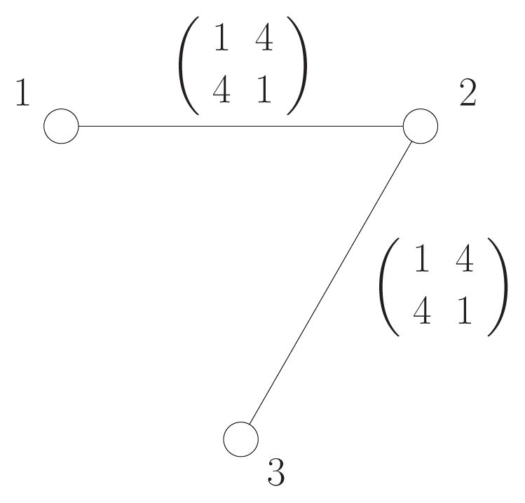
The diagram shows the graphical model and pairwise compatibility functions ψ12(x1, x2) and ψ23(x2, x3) of the distribution used in Example 3.
| (3) |
and
| (4) |
That is, .
Then, it is easy to verify for all x1 ∈ {0, 1}. Therefore, we can define max-marginals μ1(x1) = 1 for all x1 ∈ {0, 1}, i.e. and . Since μ2(x2) and μ3(x3) can be defined similarly, we obtain μi(xi) = 1 for all xi ∈ {0, 1} and i ∈ {1, 2, 3}.
Likewise, we can verify is 4/50 if x1 = x2, and 42/50 otherwise. Since we obtain the same result when maximizing under fixed (x2, x3) values, we can define μij(xi, xj) as
| (5) |
i.e. and .
In this example, we realize μi(xi) = ψi(xi) and μij(xi, xj) = ψij(xi, xj) for all i, j, and also μij(xi, xj) = ψij(xi, xj)ψi(xi)ψj(xj). This makes us easily verify that p(x) is factorized by max-marginals:
| (6) |
| (7) |
Now, assume that we are given p(x) and the max-marginals {μi, μij}. We illustrate how max-marginals can be used to compute maxx p(x). We know for some Y. The value of Y can be easily computed by comparing both sides of the equation for some specific assignment, e.g. (0, 0, 0). In this example, we obtain Y = 50 as shown in (7). Assuming x* is a MAP assignment, we have
| (8) |
Since we know and ( ) should be a maximizer of μi(xi) and μij(xi, xj), respectively, the maximum value of p(x) can be obtained simply by finding the maximum value of each μi(xi) and μij(xi, xj) without needing to find the actual assignment x*. Therefore, maxxp(x) = 42/50.
Max-marginals are also useful in finding a MAP assignment for a tree distribution50. We can easily determine a MAP assignment value for the root node of the tree by finding a value that maximizes the singleton max-marginals of the root. Then, the MAP assignment is determined for the rest of the nodes in the order of tree traversal from the root to leaves; for each pair of parent and child nodes and a given assignment for the parent node, the child node assignment is a value that maximizes the corresponding pairwise max-marginals.
For a distribution over a non-tree (cyclic) graphical model, knowing the exact max-marginals does not necessarily imply a MAP assignment or the maximum value of p(x) can be easily found. There are special cases that allow efficient computation of MAP assignments for cyclic distributions using max-marginals. For example, when each singleton max-marginals factor has a unique maximizer, the assignment consisting of these maximizers is the unique MAP assignment. More generally, an assignment that maximizes every max-marginals factor of the distribution is a MAP assignment47. Such an assignment can be more efficiently found by restricting the search to a subgraph derived from singleton factors that have multiple maximizers38. However, this search is still very large in case there are many maximizers of each singleton max-marginals factor and the subgraph is densely connected.
The ordinary max-product (also known as max-plus or min-sum) algorithm49 is an iterative algorithm that estimates a MAP assignment by propagating a series of messages along the edges of the graphical model. The algorithm exactly computes a MAP assignment for tree distributions, but it does not guarantee finding one for cyclic distributions. It is known that the ordinary max-product algorithm applied to a tree distribution can be interpreted as computing max-marginals exactly and efficiently50. For general cyclic distributions, there is no known method that efficiently computes max-marginals; it can be as expensive as the original MAP estimation problem.
Pseudo-max-marginals
Instead of attempting to compute max-marginals, Wainwright et al.47 use the notion of pseudo-max-marginals in their tree-reweighted max-product (message-passing) algorithm. Pseudo-max-marginals are defined so that they become max-marginals for each tree distribution used in the algorithm, and the original distribution is represented as a convex combination of these tree distributions.
The basic idea of the tree-reweighted max-product algorithm is to express a cyclic distribution as a convex combination of distributions over a set of spanning trees. This convex combination of tree distributions is used to upper bound the MAP probability, that is, to lower bound the energy. It can be shown that the upper bound is tight if and only if every tree distribution shares a common MAP configuration, i.e. tree agreement47. The tree-reweighted max-product algorithm tries to induce this tree agreement by factorizing each tree distribution with factors called pseudo-max-marginals and having pseudo-max-marginals converge to the max-marginals of each tree distribution.
Let us assume we use the tree-reweighted max-product algorithm with
 , a set of spanning trees of
, and some non-negative constant ρ(T) for each T ∈
such that ΣT∈
, a set of spanning trees of
, and some non-negative constant ρ(T) for each T ∈
such that ΣT∈
 ρ(T) = 1. The tree-reweighted max-product algorithm requires that every vertex and edge of
be covered by
, i.e. each vertex and edge in
is in some tree T in
such that ρ(T) > 0. Then, by construction, pseudo-max-marginals ν = {νi, νij} from the tree-reweighted max-product algorithm satisfy “ρ-reparameterization”, that is described as:
ρ(T) = 1. The tree-reweighted max-product algorithm requires that every vertex and edge of
be covered by
, i.e. each vertex and edge in
is in some tree T in
such that ρ(T) > 0. Then, by construction, pseudo-max-marginals ν = {νi, νij} from the tree-reweighted max-product algorithm satisfy “ρ-reparameterization”, that is described as:
| (9) |
where ρij is an edge coefficient such that ρij = ΣT∈
:(i,j)∈
 (T)
ρ(T) defined for all (i, j) ∈
, and ρi is a vertex coefficient such that ρi = ΣT∈
:i∈
(T)
ρ(T) defined for all (i, j) ∈
, and ρi is a vertex coefficient such that ρi = ΣT∈
:i∈
 (T)
ρ(T) defined for all i ∈
. Note that, if
is a set of spanning trees, then ρi is 1 for all i ∈
.
(T)
ρ(T) defined for all i ∈
. Note that, if
is a set of spanning trees, then ρi is 1 for all i ∈
.
A tree distribution pT(x; ν) for some T ∈
and given pseudo-max-marginals can be defined as
| (10) |
Then, we have p(x) ∝ ΠT∈
{pT(x; ν)}ρ(T) from (9). The pseudo-max-marginals ν* at convergence of the tree-reweighted max-product algorithm satisfy the “tree-consistency condition” with respect to every tree T ∈
. That is, the pseudo-max-marginals converge to the max-marginals of each tree distribution.
Example 2 (Pseudo-max-marginals)47
Let x ∈ {0, 1}3 be a random vector on a graphical model illustrated in Figure 6(a). Let , where ψi(xi) and ψij(xi, xj) are defined same as in Example 1. We define pseudo-max-marginals ν̂ as follows:
| (11) |
| (12) |
Figure 6.

Illustration of pseudo-max-marginals and ρ-reparameterization. (a) Original distribution. (b) – (d) Pseudo-max-marginals on each tree used by convex combination.
Figure (a). p(x)
Figure (b). p1(x; ν●);
Figure (c). p2(x; ν●);
Figure (d). p3(x; ν●);
Figure 6(b) – (d) illustrates the trees used for the convex combination and pseudo-max-marginals on each tree. It can be easily verified that pseudo-max-marginals on each tree are in fact max-marginals. Thus, the pseudo-max-marginals are tree-consistent. The distribution for each tree is given by (10). For example, the distribution for Figure 6(b) is
| (13) |
Then, by letting ρ(T) = 1/3 for all three trees, we obtain
| (14) |
| (15) |
from ψi(xi) = ν̂i(xi)−1/3 and ψij(xi, xj) = ν̂ij(xi, xj)2/3. This verifies the pseudo-max-marginals satisfy ρ-reparameterization as well.
TRMP
Algorithm 1 in Appendix A describes “edge-based reparameterization updates”47 defining
as a set of (not necessarily spanning) trees in
, as used by Kolmogorov51. In what follows, we will call this algorithm TRMP in short. Note that, although we define
as a set of general trees covering all vertices and edges of
, it can be easily verified that all the analyses done by Wainwright et al.47 can be applied to TRMP in exactly the same way, to show TRMP has the same properties owned by the original edge-based reparameterization updates.
TRMP can sometimes guarantee the optimality of an assignment found at convergence for cyclic distributions. Even if TRMP does not find the exact MAP assignment, we can easily compute the exact maximum value for each tree distribution at TRMP convergence since pseudo-max-marginals converge to max-marginals for each tree distribution. Then, we can combine these to get an upper bound for the original, cyclic distribution (thereby obtaining a lower bound on the energy).
We are free to choose any set of trees
and ρ(·) as long as each vertex and edge is covered by some T ∈
with ρ(T) > 0. In this work, we consistently use a set of maximal stars
 in place of
for the convenience of implementation and the simplicity in computing rotamer-pair lower bounds. A star is a tree where at most one vertex is not a leaf. We denote the center of star S as γ(S). A maximal star is a star that is not a subset of another star. Figure 7 illustrates covering a graph by a set of maximal stars; all vertices and edges of graph (a) are covered by
consisting of three maximal stars. In general, covering dense graphs such as complete graphs requires
in place of
for the convenience of implementation and the simplicity in computing rotamer-pair lower bounds. A star is a tree where at most one vertex is not a leaf. We denote the center of star S as γ(S). A maximal star is a star that is not a subset of another star. Figure 7 illustrates covering a graph by a set of maximal stars; all vertices and edges of graph (a) are covered by
consisting of three maximal stars. In general, covering dense graphs such as complete graphs requires
 (n) maximal stars. As explained in Lemma 3, computing a rotamer-pair lower bound involves solving a constrained maximization problem for each tree distribution. Therefore, using
allows us to address only
(n) maximization problems in computing a rotamer-pair lower bound. In addition, due to the structure of a star, maximization of each tree (i.e. star) distribution can be simplified to one of the four cases of (22).
(n) maximal stars. As explained in Lemma 3, computing a rotamer-pair lower bound involves solving a constrained maximization problem for each tree distribution. Therefore, using
allows us to address only
(n) maximization problems in computing a rotamer-pair lower bound. In addition, due to the structure of a star, maximization of each tree (i.e. star) distribution can be simplified to one of the four cases of (22).
Figure 7.

Example of covering a graph by maximal stars:
of (a) is completely covered by S1, S2, and S3.
Figure (a).
Figure (b). S1
Figure (c). S2
Figure (d). S3
Following the terminology of Kolmogorov51, we say ν is in a normal form if it satisfies maxr∈Ri
νi(r) = 1 for all i ∈
, and max(r,s)∈Ri×Rj
νij (r, s) = 1 for all (i, j) ∈
. In what follows, we assume ν of Algorithm 1 is always in a normal form. Then, from (2) and (9), and by introducing a positive constant νc, we obtain the following equation:
| (16) |
Table I.
Test case facts. Each column represents (1) No.: case number, (2) Model: model system, (3) Region: protein regions being considered, (4) AA: type of amino acids offered for design positions, (5) Lib: types of rotamer library used, (6) n: number of positions, (7) nD: number of design positions, (8) w: number of mobile water molecules considered, (9) Σ|Ri|: total number of rotamers, (10) Pairs: total number of rotamer pairs, (11) logconf: , (12) Solved by: methods that solved the case (“Limited DEE” implies the case was solved by both BroMAP and DEE/A*, but only DEE-gp was necessary for BroMAP. “Bro” and “DEE” abbreviate BroMAP and DEE/A*, respectively).
| No. | Model | Region | AA | Lib | n | nD | w | Σ|Ri| | Pairs | logconf | Solved by |
|---|---|---|---|---|---|---|---|---|---|---|---|
| 1 | fn3 | core | HP | REG | 14 | 14 | 0 | 743 | 2.5E5 | 50.2 | Limited DEE |
| 2 | fn3 | core++ | HP | REG | 20 | 20 | 0 | 1,778 | 1.5E6 | 83.7 | Bro & DEE |
| 3 | fn3 | core++ | HP | REG | 23 | 23 | 0 | 1,894 | 1.7E6 | 94.1 | Bro & DEE |
| 4 | fn3 | core++ | HP | REG | 25 | 25 | 0 | 2,048 | 2.0E6 | 102.9 | Bro & DEE |
| 5 | fn3 | core++ | HP | REG | 27 | 27 | 0 | 2,083 | 2.1E6 | 108.6 | Bro & DEE |
| 6 | fn3 | core | HP | EXP | 14 | 14 | 0 | 8,774 | 3.5E7 | 82.4 | Limited DEE |
|
| |||||||||||
| 7 | D44.1 | int | A | REG | 7 | 4 | 0 | 476 | 8.5E4 | 21.6 | Limited DEE |
| 8 | D44.1 | int | A | REG | 7 | 7 | 0 | 822 | 2.8E5 | 28.7 | Limited DEE |
| 9 | D44.1 | int | A | REG | 8 | 8 | 0 | 965 | 4.0E5 | 33.4 | Bro & DEE |
| 10 | D44.1 | int | A | REG | 9 | 9 | 0 | 1,019 | 4.5E5 | 37.1 | Bro & DEE |
| 11 | D44.1 | int | A | REG | 10 | 10 | 0 | 1,133 | 5.6E5 | 40.6 | Bro & DEE |
| 12 | D44.1 | int | A | REG | 11 | 11 | 0 | 1,376 | 8.4E5 | 46.4 | Bro |
| 13 | D44.1 | int | A | REG | 16 | 14 | 2 | 2,020 | 1.9E6 | 70.1 | None |
| 14 | D44.1 | int | A | EXP | 7 | 4 | 0 | 5,026 | 9.5E6 | 36.4 | Limited DEE |
| 15 | D44.1 | int | A | EXP | 7 | 5 | 0 | 7,019 | 1.9E7 | 39.9 | Bro & DEE |
| 16 | D44.1 | int | A | EXP | 7 | 6 | 0 | 7,910 | 2.6E7 | 42.9 | Bro |
|
| |||||||||||
| 17 | D44.1 | int | A | EXP | 7 | 7 | 0 | 8,771 | 3.2E7 | 42.9 | Bro |
| 18 | D1.3 | int | A | REG | 6 | 4 | 2 | 450 | 8.3E4 | 21.7 | Limited DEE |
| 19 | D1.3 | int | A | REG | 11 | 8 | 3 | 767 | 2.6E5 | 38.5 | Limited DEE |
| 20 | D1.3 | int | A | REG | 23 | 7 | 9 | 1,618 | 1.2E6 | 78.8 | Limited DEE |
| 21 | D1.3 | int | A | EXP | 6 | 4 | 2 | 3,599 | 4.8E6 | 28.7 | Limited DEE |
| 22 | D1.3 | int | A | EXP | 7 | 5 | 2 | 3,616 | 4.8E6 | 28.7 | Limited DEE |
| 23 | D1.3 | int | A | EXP | 8 | 6 | 2 | 4,070 | 6.3E6 | 34.4 | Bro & DEE |
| 24 | D1.3 | int | A | EXP | 11 | 4 | 3 | 4,612 | 8.0E6 | 42.6 | Bro & DEE |
| 25 | D1.3 | int | A | EXP | 11 | 6 | 3 | 4,987 | 9.7E6 | 45.1 | Bro & DEE |
| 26 | D1.3 | int | A | EXP | 11 | 7 | 3 | 5,461 | 1.2E7 | 47.4 | Bro & DEE |
| 27 | D1.3 | int | A | EXP | 11 | 7 | 3 | 5,891 | 1.4E7 | 50.5 | Bro |
| 28 | D1.3 | int | A | EXP | 11 | 8 | 3 | 6,365 | 1.7E7 | 52.8 | Bro |
| 29 | D1.3 | core | H | REG | 16 | 16 | 0 | 342 | 5.4E4 | 44.1 | Limited DEE |
| 30 | D1.3 | core | H | REG | 20 | 20 | 0 | 430 | 8.6E4 | 54.6 | Limited DEE |
| 31 | D1.3 | core | H | REG | 26 | 26 | 0 | 503 | 1.2E5 | 66.7 | Limited DEE |
| 32 | D1.3 | core | H | REG | 34 | 34 | 0 | 567 | 1.5E5 | 81.4 | Limited DEE |
| 33 | D1.3 | core | HP | REG | 16 | 16 | 0 | 980 | 4.4E5 | 59.5 | Bro & DEE |
| 34 | D1.3 | core | HP | REG | 20 | 20 | 0 | 1,228 | 7.1E5 | 74.1 | Bro & DEE |
| 35 | D1.3 | core | HP | REG | 26 | 26 | 0 | 1,431 | 9.7E5 | 92.3 | Bro & DEE |
| 36 | D1.3 | core | HP | REG | 34 | 34 | 0 | 1,582 | 1.2E6 | 112.7 | Bro & DEE |
| 37 | D1.3 | core | H | EXP | 13 | 13 | 0 | 1,844 | 1.5E6 | 56.3 | Bro & DEE |
| 38 | D1.3 | core | H | EXP | 16 | 16 | 0 | 2,734 | 3.5E6 | 75.7 | Bro |
| 39 | D1.3 | core | H | EXP | 20 | 20 | 0 | 3,370 | 5.3E6 | 91.8 | Bro |
| 40 | D1.3 | core | H | EXP | 26 | 26 | 0 | 3,894 | 7.1E6 | 111.6 | Bro |
| 41 | D1.3 | core | H | EXP | 34 | 34 | 0 | 4,444 | 9.4E6 | 142.0 | Bro |
|
| |||||||||||
| 42 | epo | int | A | REG | 5 | 5 | 0 | 466 | 7.1E4 | 16.6 | Limited DEE |
| 43 | epo | int | A | REG | 6 | 6 | 0 | 419 | 6.8E4 | 17.0 | Limited DEE |
| 44 | epo | int | A | REG | 11 | 11 | 0 | 1,005 | 4.4E5 | 39.4 | Bro & DEE |
| 45 | epo | int | A | REG | 21 | 11 | 3 | 1,503 | 1.0E6 | 67.5 | Bro & DEE |
| 46 | epo | int | A | REG | 21 | 15 | 3 | 1,999 | 1.9E6 | 79.6 | Bro |
| 47 | epo | int | A | REG | 21 | 18 | 3 | 2,138 | 2.1E6 | 87.5 | None |
| 48 | epo | int | A | EXP | 5 | 5 | 0 | 5,001 | 8.4E6 | 26.5 | Limited DEE |
| 49 | epo | int | A | EXP | 6 | 6 | 0 | 4,170 | 6.8E6 | 26.3 | Bro & DEE |
| 50 | epo | int | A | EXP | 8 | 8 | 0 | 7,544 | 2.3E7 | 46.4 | Bro & DEE |
| 51 | epo | int | A | EXP | 9 | 9 | 0 | 8,724 | 3.2E7 | 53.4 | Bro & DEE |
| 52 | epo | core | H | REG | 17 | 17 | 0 | 291 | 3.9E4 | 43.5 | Limited DEE |
| 53 | epo | core | H | REG | 22 | 22 | 0 | 395 | 7.4E4 | 58.1 | Limited DEE |
| 54 | epo | core | H | REG | 28 | 28 | 0 | 433 | 8.9E4 | 65.4 | Limited DEE |
| 55 | epo | core | H | REG | 33 | 33 | 0 | 573 | 1.6E5 | 82.7 | Limited DEE |
| 56 | epo | core | H | REG | 41 | 41 | 0 | 727 | 2.6E5 | 103.3 | Limited DEE |
| 57 | epo | core | HP | REG | 17 | 17 | 0 | 827 | 3.2E5 | 60.1 | Bro & DEE |
| 58 | epo | core | HP | REG | 22 | 22 | 0 | 1,103 | 5.8E5 | 79.9 | Bro & DEE |
| 59 | epo | core | HP | REG | 28 | 28 | 0 | 1,208 | 7.0E5 | 92.6 | Bro & DEE |
| 60 | epo | core | HP | REG | 33 | 33 | 0 | 1,615 | 1.3E6 | 115.9 | Bro & DEE |
| 61 | epo | core | HP | REG | 36 | 36 | 0 | 1,827 | 1.6E6 | 128.4 | Bro |
| 62 | epo | core | HP | REG | 38 | 38 | 0 | 1,956 | 1.9E6 | 136.6 | Bro |
| 63 | epo | core | HP | REG | 41 | 41 | 0 | 1,999 | 1.9E6 | 143.1 | Bro |
| 64 | epo | core | H | EXP | 17 | 17 | 0 | 2,307 | 2.4E6 | 73.5 | Limited DEE |
| 65 | epo | core | H | EXP | 22 | 22 | 0 | 3,006 | 4.2E6 | 99.0 | Bro & DEE |
| 66 | epo | core | H | EXP | 28 | 28 | 0 | 3,213 | 4.8E6 | 111.1 | Bro & DEE |
| 67 | epo | core | H | EXP | 33 | 33 | 0 | 4,322 | 8.9E6 | 140.0 | Bro |
| 68 | epo | core | H | EXP | 41 | 41 | 0 | 5,712 | 1.6E7 | 175.0 | None |
The value of νc can be computed by comparing both sides of (16) for any assignment x ∈
. Equivalently, p(x) can be expressed as follows:
| (17) |
Bounding the GMEC energy with TRMP
We also make heuristic use of TRMP to obtain upper bounds for the GMEC energy. At convergence of TRMP, we occasionally find an exact MAP configuration. TRMP provides an easy evaluation condition called optimum specification (OS) criterion such that an assignment is guaranteed to be a MAP configuration if it satisfies the OS criterion. However, such an assignment may not exist for a given reparameterization or it could be computationally expensive to find. Therefore, in our upper bounding, instead of trying to find an assignment that satisfies the OS criterion, we simply find an assignment that maximizes the tree distribution for some star S ∈
at TRMP convergence, using dynamic programming50. Another possible upper-bounding method is to randomly pick a maximizer for each singleton max-marginals at TRMP convergence regardless of the trees. Although neither of these procedures guarantees the quality of the upper bounds, the resulting upper bounds are empirically close to the optimal values. The procedures can be repeated for different trees or different random selection of maximizers to improve the upper bounds.
A lower bound for the GMEC energy minx e(x) can be easily obtained at the convergence of TRMP with the following lemma:
Lemma 1
When ν and νc of (17) in a normal form satisfy the tree-consistency condition, the MAP probability is upper bounded by
| (18) |
Therefore, the GMEC energy minx
e(x) is lower bounded by minx
e(x) ≥ − ln νc from (2). This lower bound of the GMEC energy is independent of the normalization constant Z because, in (16), the product ΠS∈
pS(x; ν) purely depends on the normalized pseudo-max-marginals, that are generated without any reference to Z. Note that Lemma 1 is true not only for star covers but for general tree covers.
Example 3
To upper bound maxx p(x) using Lemma 1 and the pseudo-max-marginals given in Example 2, we first need to normalize pairwise pseudo-max-marginals. Since the maximum value of ν̂ij(xi, xj) for all (i, j) are 8, normalized pairwise pseudo-max-marginals are as follows:
| (19) |
Singleton pseudo-max-marginals are already in a normal form. Given the normalized pseudo-max-marginals, and p(x), we can compute νc/Z = 64/98 from (17). Note that νc/Z is computed instead of νc in this example because we are given p(x), but not e(x). Then, by Lemma 1, the upper bound of the MAP probability is 64/98. It is easy to see maxx
p(x) is equal to 16/98 attained by any of (x1, x2, x3) = (0, 0, 1), (0, 1, 0), etc. The upper bound of the MAP probability (thereby the resulting lower bound of the GMEC energy) is not tight in this example, but the quality of bounds from Lemma 1 can be stronger depending on pseudo-max-marginals from TRMP. In this example, on the other hand, a tight lower-bound of p(x) (therefore a tight upper-bound of the GMEC energy) is easily obtained by finding a MAP assignment for any of the trees in
. For instance, (x1, x2, x3) = (0, 1, 0) is a MAP assignment for tree distribution p1(x; ν), and also for p(x).
Elimination by TRMP lower bounds
We can exploit the tree-consistency of ν at TRMP convergence in computing various lower bounds for a set of conformations. If a lower bound greater than a global upper-bound U is obtained, we can eliminate corresponding conformations from the subproblem while conserving the inequality relation between the minimum energy of the subproblem and U. We make a more precise argument for what we call rotamer-pair elimination and rotamer elimination as follows. Let P̃ be the set of flagged rotamer pairs in the subproblem of our interest. Then, given conformational space
, we define
 (
, P̃) as the set of all legal conformations containing no flagged rotamer pairs.
(
, P̃) as the set of all legal conformations containing no flagged rotamer pairs.
1. rotamer-pair elimination: suppose we have a lower-bound LB(ζr, ηs) of the minimum conformational energy for {x|(xζ, xη) = (r, s)}, the set of all conformations including (ζr, ηs), such that min{x|(xζ,xη)=(r,s)}
e(x) ≥ LB(ζr, ηs) > U. Elimination of (ζr, ηs) can be represented by the set of pair-flags P̃′ = P̃ ∪ ζr, ηs). We know minx∈
 (
,P̃′)
e(x) is prunable if and only if minx∈
(
,P̃)
e(x) is prunable. Therefore, we use P̃′ as the updated set of pair flags.
(
,P̃′)
e(x) is prunable if and only if minx∈
(
,P̃)
e(x) is prunable. Therefore, we use P̃′ as the updated set of pair flags.
2. rotamer elimination: suppose we have a lower-bound LB(ζr) of the minimum conformational energy for {x|xζ = r}, the set of all conformations including ζr, such that min{x|xζ= r}
e(x) ≥ LB(ζr) > U. Elimination of ζr can be represented by the set of pair-flags P̃′= P̃ ∪ {(ζr, js)|s ∈ Rj, j ∈
, j ≠ ζ}, which includes all rotamer pairs stemming from ζr. Again, we know min x∈
(
,P̃′)
e(x) is prunable if and only if minx∈
(
,P̃)
e(x) is prunable. Therefore, we use P̃′ as the updated set of pair flags. In both cases, the optimal value of minx∈
(
,P̃)
e(x) does not change if minx∈
(
,P̃)
e(x) ≤ U.
The lower-bounds LB(ζr) and LB(ζr, ηs) can be, for example, obtained by directly solving an LP relaxation of the ILP given in Appendix B. However, solving LP may not be practical when the problem size is large. In addition, solving LP for every rotamer or rotamer pair will multiply the lower-bounding time by the number of rotamers or rotamer pairs. Here, we use upper-bounding inequalities for the singleton and pairwise max-marginals to obtain lower bounds for minimum conformational energies of rotamers and rotamer pairs. Such lower bounds are at best as tight as the bounds from solving the LP discussed in Appendix B47, but requires computation time for one TRMP run until convergence (no guaranteed time bound) plus post-processing time at most cubic of the problem size. The rest of this section explains how we can efficiently compute the rotamer and rotamer-pair lower bounds.
We have the following lemma on upper-bounding the singleton max-marginals:
Lemma 2
When ν and νc of (17) in a normal form satisfy the tree-consistency condition, it is true for all r ∈ Rζ, ζ ∈
that
| (20) |
Example 4
From Lemma 2 and the normalized pseudo-max-marginals given in Example 3, we find an upper bound for the maximum probability of p(x) when x1 = 0 as (νc/Z)ν1(0)1/3 = 64/98 × 11/3. The bound is not tight because max{x|x1=0} p(x) = 16/98, but the tightness may change depending on the pseudo-max-marginals from TRMP. Even when the resulting bound is not tight, it could be still strong enough to eliminate the corresponding rotamer through comparison against a global upper-bound U.
Lemma 2 combined with (2) provide a rotamer lower-bound LB(ζr) for each r ∈ Rζ and ζ ∈
as min{x|xζ=r}
e(x) ≥ LB(ζr) = − ln νc − ρζ ln νζ(r).
To upper bound the pairwise max-marginals, we use the general inequality
| (21) |
The maximization problem max{x|xζ =r,xη=s} pS(x; ν) can be easily solved using the following lemma:
Lemma 3
When ν and νc of (17) in a normal form satisfy the tree-consistency condition,
| (22) |
Example 5
Let us bound max{x|(x1,x2)=(0,0)} p(x) using the normalized pseudo-max-marginals given in Example 3. As discussed above, we have to solve maximization problem for each star:
- p1(x; ν) and p3(x; ν) (Figure 6(b) and 6(d)): this corresponds to the third case of (22). Therefore,
By combining the above results in (21), we obtain
| (24) |
This bound is tight from max{x|(x1,x2)=(0,0)} p(x) = 16/98 attained by x3 = 1. Note that the same pseudo-max-marginals that yielded weak upper bounds in Examples 3 and 4, led to a tight upper bound for the rotamer pair, a more constrained bounding problem.
LB(ζr, ηs), a lower bound for the minimum conformation energy of rotamer-pair (ζr, ηs), is given by LB(ζr, ηs) = − ln νc − ΣS∈
 ρS ln max{x|xζ=r,xη=s}
pS(x; ν).
ρS ln max{x|xζ=r,xη=s}
pS(x; ν).
Note that there can be at most
(n) stars that correspond to the fourth case of (22) for each position pair (ζ, η). If we let nrot be the average number of rotamers per position, the maximization problem corresponding to the fourth case of (22) requires
(nrot) operations. Therefore, it will take
(nrotn) post-processing operations to compute an upper bound for each rotamer pair using Lemma 3.
In computing the rotamer lower bound for a rotamer ζr, we can also use pair-flags information to obtain a lower bound, LB′(ζr), for the constrained problem min{x∈
(
,P̃)|xζ =r}
e(x). If we have LB′(ζr) > U, then conformations, {x ∈
(
, P̃)|xζ = r} can be excluded from the search space. This is equivalent to eliminating rotamer ζr because all conformations containing xζ = r are in effect excluded. Computing LB′(ζr) will take additional polynomial time compared to LB(ζr), but it is particularly advantageous to leverage the pair flags when there exist a large number of flagged rotamer pairs. We used a simple search-based method to compute LB′(ζr) as follows; let p̂ = ΠS∈
[max{x∈
(
,P̃)|xζ=r}
pS(x; ν)ρ(S) for tree-consistent ν in a normal form. Then, it is easy to see (νc/Z)p̂ is an upper bound of max{x∈
(
, P̃)|xζ=r}
p(x). If we use a naive search, it will take
post-processing comparison operations to compute max{x∈
(
,P̃)|xζ=r}pS(x; ν). Therefore, it takes
post-processing time to exactly compute p̂. Finally, the rotamer lower bound is computed as LB′(ζr) = − ln νc − ln p̂.
Results and Discussions
We performed computational experiments to evaluate the performance of BroMAP. We used a set of various protein design cases to measure and compare the running times of BroMAP and a fast implementation of DEE/A* that includes most of the state-of-art techniques26. In the following, to distinguish the modified version of DEE used in BroMAP from the DEE used in DEE/A*, we will call the former as DEE-gp (DEE for general pair flags). The two main questions we are interested in investigating with the experiments are (1) whether BroMAP can solve design cases previously unsolved by DEE/A*, and (2) whether we can use BroMAP generally as an alternative to DEE/A* without being restricted to specific types of design cases. Although we are mainly interested in the overall performance of BroMAP here, Hong and Lozano-Pérez52 evaluate the effectiveness of our pruning method by comparing it against linear programming.
DEE/A* implementation
We used an in-house implementation of DEE/A* written in the C programming language53. DEE/A* was performed with the following options and order:
Eliminate singles using Goldstein’s condition21. Repeat until elimination is unproductive.
Eliminate singles using split flags (s = 1)24. Repeat until elimination is unproductive.
Do logical singles-pairs elimination22.
Eliminate pairs using Goldstein’s condition with one magic bullet23.
Do logical singles-pairs elimination.
If unification is possible, do unification21, and go to (1).
Do A*46.
For unification, the pair of positions that has the largest fraction of flagged rotamer pairs is picked. However, because the energy terms and pair flags must be stored in machine memory, we capped the total number of rotamers that would result to be no greater than a unification option Cuni. Therefore, any pair of positions that would create a larger number of rotamers when unified than Cuni was not considered, and the pair with the next-largest fraction of flagged rotamer pairs was considered. We experimented with different values of Cuni, i.e. 6,000, 8,000, 10,000, 12,000, and 14,000, to obtain the best running time for each test case. Note that this gives DEE/A*, the competing method an advantage over BroMAP in comparing their running times, because it will give better DEE/A* times than consistently using one of the Cuni values. Increasing Cuni and thus the allowance for large unification can facilitate solving otherwise difficult or unsolvable cases. However, for small to medium cases, larger values of Cuni often result in slower solution times.
Our DEE implementation uses a full table of energies. That is, if there are rotamers in the problem, DEE allocates memory for q2 floating point numbers.
When the DEE/A* procedure described above using various Cuni values failed to solve a test case, we also tried singles-elimination using split flags with s = 2 instead of s = 1, or allowed the number of magic bullets to increase up to the number of positions.
BroMAP implementation
BroMAP was implemented in C++. We used the PICO-library54 for the BnB framework. The PICO-library provides the data structures and methods to create/delete nodes and to search the tree. It also provides procedure skeletons, for instance, for upper/lower-bounding methods.
In BroMAP, we restricted the amount of effort spent by DEE-gp instead of allowing it to keep iterating singles/pairs-flagging and unification until it finally solved the subproblem. This was done by limiting the maximum number of iterations of singles/pairs-flagging and also by using a smaller fixed Cuni value for unification than those used by DEE/A*.
Other than performing DEE-gp and TRMP bounding for each subproblem, we also allowed rotamer-contractions52. Rotamer-contraction reduces the size of a subproblem by grouping similar rotamers at a residue position as a cluster and replacing the cluster by a new single rotamer. It also defines the pairwise energies for the new rotamer so that the optimal value of the reduced subproblem is always a lower bound of the optimal value of the subproblem before the rotamer-contraction. Rotamer-contraction was iteratively performed until we obtained a lower bound greater than U or the number of executed rotamer-contractions reached a pre-determined limit. We used a heuristic boundability index (BI) multiplied by a positive integer Prc as such limits. The BI for a specific node is equal to the number of ‘high’ branches on the path from the root to the node. For example, in the search tree of Figure 1, assuming the BI of the root node is equal to 0, BI’s are 0 for nodes 1, 3, 5, 7, 9, and 1 for nodes 2, 4, 6, 8, 11, and 2 for node 10. In these experiments, we let Prc = 16 after exploring the overall effect of different values of Prc on running times of BroMAP.
In case rotamer-contractions were performed multiple times in bounding a subproblem as described above, we also performed additional DEE-gp and TRMP periodically on the subproblem reduced by rotamer-contractions. After every PDEE consecutive rotamer-contractions, we applied DEE-gp to see if we could solve the reduced problem or only to flag more rotamers or rotamer pairs. TRMP was also run until convergence after every PTRMP consecutive rotamer-contractions to compute a lower bound for the subproblem or to flag rotamers or rotamer-pairs using the TRMP lower bounds. In this experiment, we let PDEE = 8, and PTRMP = 16.
Along the first depth-first dive, that is, until we exactly solve a subproblem for the first time, we performed only DEE-gp, TRMP bounding, and subproblem splitting, once respectively, but did not use any rotamer-contraction. As with DEE/A*, BroMAP also used the A* search algorithm when DEE-gp could not eliminate any more rotamers or rotamer pairs and the subproblem was considered small, i.e. contained less than 200,000 rotamer pairs.
The BroMAP implementation needs to hold TRMP data, whose size is of the order of the number of rotamer pairs. This corresponds to floating point numbers, and is roughly half the memory required by DEE/A*. Since BroMAP also performs DEE-gp, it requires additional memory of floating point numbers for the full DEE energy table. Therefore, the maximum memory requirement of BroMAP is floating point numbers, which is roughly 1.5 times larger than that of DEE/A*.
Platform
We used a Linux workstation with two dual-core 2 GHz AMD Opteron 246 processors and 2 Gbytes of memory for the experiment. The C/C++ codes for BroMAP and DEE/A* were compiled using Intel C/C++ Compiler Version 9.1 for Linux. During compile, OpenMP directives were enabled to parallelize the execution of DEE, DEE-gp, and TRMP over two CPU cores. All other procedures, including A*, were executed over a single core. Note that BroMAP or DEE/A* was allowed to use the whole system memory but only one processor at a time.
Test cases
We used 68 test cases whose energy files are smaller than 300 Mbytes. An energy file contains floating point numbers representing singleton and pairwise energies. We found energy files larger than 300 Mbytes are not handled well with the current implementation of BroMAP on our workstation due to the memory requirement of BroMAP.
We used three different model systems in obtaining test cases:
FN3: derived from protein 10 Fn3, the tenth human fibronectin type III domain55. It is a 94-residue β-sheet protein with an immunoglobulin-like fold. Besides its natural in vivo role, the protein has been engineered as an antibody mimic to bind with high affinity and specificity to arbitrary protein targets.
D44.156 and D1.357: antibodies that bind to hen egg-white lysozyme (HEL), though they bind different HEL epitopes. Each has low nanomolar binding affinity, and was originally isolated after murine immunization. For the D1.3 core designs, we redesigned the core of the lysozyme protein, absent of the antibody.
EPO: human erythropoietin (Epo) protein complexed to its receptor (EpoR)58. One Epo binds to two EpoR with one high-affinity and one low-affinity binding sites. Our EPO interface designs addressed the high-affinity binding site while our core designs addressed the core of the EpoR from the high-affinity site.
Each case corresponds to one of three types of protein regions:
INT: protein–protein binding interface.
CORE: protein core, i.e. side chains that are not solvent-exposed.
CORE++: protein core plus boundary positions that are partially exposed to solvent.
We varied the types of amino acids offered at design positions of each case as follows:
H: hydrophobic amino acids (A, F, G, I, L, M, W, V).
HP: hydrophobic plus polar amino acids (A, F, G, I, L, M, W, V, H, N, Q, S, T, Y).
A: all type of amino acids, excluding proline and cysteine.
For CORE, we used both H and HP, and for CORE++, we used HP (with both neutral tautomers of histidine allowed in each case). For INT, we used A, and allowed both neutral tautomers and the protonated form of histidine. For all designs, if the wild-type amino acid was not part of the library, it was added at that position. For some test cases, the total number of positions in the search was greater than the number of design positions. At these other positions, the native amino-acid type was retained and its conformation was varied.
Each case was made using one of two different rotamer libraries:
REG: standard rotamer library. This is based on the backbone-independent May 2002 library59. This library was supplemented with three histidine rotamers for an unsampled ring flip, and two asparagine rotamers to increase sampling of the final dihedral angle rotation.
EXP: expanded rotamer library. This was created by expanding both χ1 and χ2 of rotamers in REG by ±10°. The hydroxyls of serine, threonine, and tyrosine were sampled every 30 degrees. For some INT cases of D1.3, D44.1, and EPO, crystallographic water molecules were allowed conformational freedom. The oxygen atom location was fixed to that of the crystal structure and the hydrogen atoms were placed to create 60 symmetric water molecule rotations.
For all libraries and cases, each crystallographic wild-type rotamer was added in a position-specific manner to the library, using the complete Cartesian representation of the side chain, rather than just the dihedral angles.
The singleton/pairwise energies of rotamers were computed using the energy function of CHARMM PARAM22 all-atom parameter set with no cut-offs for non-bonded interactions and a 4r distance-dependent dielectric constant. All energy terms were used (bond, angle, Urey-Bradley, dihedral, improper, Lennard-Jones, and electrostatic). Rotamers that clashed with the fixed protein regions were eliminated during case generation if their singleton energies were greater than the smallest singleton energy at that position by at least 50 kcal/mol. Further details on design methods and test case construction can be found from Lippow et al.60
Table I lists composition and problem-size information of each test case. Its last column also summarizes the experimental results presented in the following.
Running time comparison
Among the 68 cases, BroMAP solved 65 cases within the 7-days allowed time whereas DEE/A* solved 51 cases for the same allowed time. There were no cases DEE/A* solved but BroMAP was not able to solve. The 14 cases solved by BroMAP but not by DEE/A* suggest that BroMAP can be an alternative to DEE/A* for hard design cases where DEE/A* performs poorly.
Among the 51 cases solved by both BroMAP and DEE/A*, solving 23 cases by BroMAP required only the DEE-gp part of BroMAP. Since BroMAP only acted as a light DEE for these cases, comparing the running times of BroMAP and DEE/A* on them is not meaningful. After eliminating these 23 cases, we are left with 28 cases for which we are interested in comparing the running times of BroMAP and DEE/A*. The running times for these 28 cases are shown in Table II. Additionally, the table lists results for 14 cases that only BroMAP solved.
Table II.
Results of solving the non-“Limited DEE” cases with BroMAP and DEE/A* (cases solved by limited DEE are not presented). Columns (1) No.: case number, (2) Bro: BroMAP solution time in seconds, (3) DEE: DEE/A* solution time in seconds, (4) T-Br: total number of branchings (i.e. splits), (5) F-Br: number of branchings during the first depth-first dive, (6) Skew: skewness of the search tree defined as , (7) F-Ub: U - OP T, i.e. difference between the upper bound from the first depth-first dive and the GMEC energy, (8) Leaf: Σi log10 |Ri| of the node at the end of the first depth-first dive, (9) Rdctn: average reduction of Σi log10 |Ri| during the first depth-first dive, i.e. (logconf-Leaf)/(F-Br), where logconf is defined in Table I, (10) RC: number of rotamer-contractions performed, (11) %DE: BroMAP time percentage used for DEE-gp, (12) %A*: BroMAP time percentage used for A*, (13) %TR: BroMAP time percentage used for TRMP. Note that columns 11 to 13 may not sum to 100% because of time spent on rotamer-contraction and overhead of using the branch-and-bound framework.
| No. | Bro | DEE | T-Br | F-Br | Skew | F-Ub | Leaf | Rdctn | RC | %DE | %A* | %TR |
|---|---|---|---|---|---|---|---|---|---|---|---|---|
| 2 | 2.6E3 | 3.1E4 | 31 | 25 | 0.90 | 0.49 | 30.7 | 2.12 | 36 | 42.8 | 0.3 | 56.3 |
| 3 | 2.4E3 | 2.3E4 | 31 | 26 | 0.93 | 0.49 | 27.7 | 2.55 | 32 | 46.2 | 0.6 | 52.6 |
| 4 | 2.8E3 | 1.3E4 | 23 | 23 | 1 | 0 | 33.7 | 3.01 | 0 | 43.9 | 0.3 | 55.5 |
| 5 | 2.7E3 | 2.1E4 | 26 | 26 | 1 | 0.55 | 27.4 | 3.12 | 0 | 37.2 | 0.4 | 62.2 |
| 9 | 1.2E2 | 4.8E2 | 3 | 3 | 1 | 0 | 27.6 | 1.93 | 0 | 8.9 | 74.1 | 17.0 |
| 10 | 4.6E2 | 1.3E3 | 13 | 10 | 0.75 | 0.37 | 26.9 | 1.02 | 74 | 7.6 | 70.4 | 14.4 |
| 11 | 5.7E3 | 3.5E4 | 109 | 17 | 0.81 | 0.36 | 26.2 | 0.85 | 663 | 3.8 | 78.9 | 11.2 |
| 15 | 2.9E2 | 3.5E2 | 0 | 0 | NA | 0 | NA | NA | 0 | 94.6 | 0.4 | 4.7 |
| 23 | 1.5E2 | 2.6E2 | 0 | 0 | NA | 0 | NA | NA | 0 | 86.7 | 0 | 12.6 |
| 24 | 3.2E2 | 3.1E2 | 4 | 4 | 1 | 0 | 25.3 | 4.33 | 0 | 62.3 | 15.1 | 21.6 |
| 25 | 2.9E2 | 1.2E3 | 0 | 0 | NA | 0 | NA | NA | 0 | 89.6 | 0 | 10.4 |
| 26 | 1.4E3 | 1.7E3 | 11 | 11 | 1 | 0.89 | 29.2 | 1.65 | 0 | 46.1 | 0.4 | 53.2 |
| 33 | 4.1E2 | 2.1E3 | 13 | 13 | 1 | 0 | 27.9 | 2.43 | 0 | 34.7 | 4.5 | 59.8 |
| 34 | 1.1E3 | 3.7E3 | 19 | 19 | 1 | 0 | 30.0 | 2.32 | 0 | 32.2 | 2.7 | 64.8 |
| 35 | 2.8E3 | 4.1E4 | 21 | 21 | 1 | 0 | 28.7 | 3.03 | 0 | 50.7 | 0.6 | 48.6 |
| 36 | 4.6E3 | 2.3E4 | 25 | 25 | 1 | 0 | 27.9 | 3.39 | 0 | 53.2 | 0.7 | 45.9 |
| 37 | 2.5E2 | 2.5E2 | 0 | 0 | NA | 0 | NA | NA | 0 | 76.0 | 2.4 | 21.2 |
| 44 | 2.2E2 | 3.8E1 | 8 | 6 | 0.71 | 0.54 | 28.2 | 1.87 | 17 | 8.2 | 75.5 | 14.1 |
| 45 | 8.8E2 | 2.0E2 | 8 | 8 | 1 | 0 | 26.2 | 5.16 | 8 | 48.6 | 23.8 | 25.4 |
| 49 | 3.3E2 | 5.0E2 | 4 | 4 | 1 | 0 | 19.8 | 1.63 | 0 | 51.1 | 11.5 | 37.5 |
| 50 | 1.2E3 | 1.1E3 | 7 | 7 | 1 | 0 | 22.3 | 3.44 | 12 | 72.2 | 7.0 | 17.1 |
| 51 | 5.7E4 | 2.8E5 | 666 | 25 | 0.85 | 0.58 | 27.6 | 1.03 | 5,656 | 16.7 | 21.2 | 41.8 |
| 57 | 4.6E1 | 2.7E2 | 0 | 0 | NA | 0 | NA | NA | 0 | 84.8 | 0 | 15.2 |
| 58 | 1.5E3 | 1.0E3 | 19 | 19 | 1 | 0 | 28.8 | 2.69 | 0 | 42.5 | 0.2 | 57.1 |
| 59 | 4.4E2 | 4.0E3 | 0 | 0 | NA | 0 | NA | NA | 0 | 70.6 | 0 | 29.1 |
| 60 | 1.5E4 | 4.6E4 | 32 | 32 | 1 | 0 | 37.3 | 2.46 | 0 | 30.1 | 0.1 | 69.7 |
| 65 | 4.6E3 | 1.7E3 | 15 | 15 | 1 | 0 | 22.7 | 5.09 | 0 | 61.9 | 0 | 37.8 |
| 66 | 7.7E3 | 2.4E3 | 15 | 15 | 1 | 0 | 33.9 | 5.15 | 0 | 67.2 | 0 | 32.6 |
|
| ||||||||||||
| Cases below were solved by BroMAP only. | ||||||||||||
|
| ||||||||||||
| 12 | 2.0E5 | NA | 2773 | 23 | 0.82 | 7.11 | 26.2 | 0.88 | 3.9E4 | 6.0 | 59.1 | 20.1 |
| 16 | 3.5E3 | NA | 12 | 11 | 0.91 | 0 | 23.6 | 1.75 | 30 | 41.7 | 6.0 | 49.3 |
| 17 | 1.1E5 | NA | 298 | 21 | 0.84 | 3.35 | 26.7 | 0.77 | 2,576 | 17.7 | 28.1 | 32.7 |
| 27 | 8.0E3 | NA | 23 | 23 | 1 | 0 | 27.8 | 0.99 | 13 | 32.2 | 1.1 | 66.4 |
| 28 | 2.1E4 | NA | 175 | 25 | 0.91 | 0 | 28.0 | 0.99 | 1,168 | 23.8 | 8.5 | 57.9 |
| 38 | 1.4E4 | NA | 155 | 31 | 0.87 | 0.50 | 30.2 | 1.47 | 571 | 30.9 | 0.4 | 62.8 |
| 39 | 1.2E5 | NA | 572 | 43 | 0.85 | 0 | 27.4 | 1.50 | 4,791 | 30.4 | 0.1 | 58.4 |
| 40 | 1.8E5 | NA | 293 | 43 | 0.81 | 0 | 29.6 | 1.91 | 2,440 | 35.9 | 0 | 56.1 |
| 41 | 2.1E5 | NA | 364 | 41 | 0.85 | 0 | 33 | 2.66 | 2,771 | 34.2 | 0 | 57.5 |
| 46 | 5.0E5 | NA | 2675 | 36 | 0.69 | 8.28 | 27.8 | 1.44 | 1.4E5 | 18.8 | 18.8 | 35.3 |
| 61 | 2.8E4 | NA | 55 | 49 | 0.96 | 0.36 | 28.2 | 2.04 | 15 | 49.0 | 0 | 50.8 |
| 62 | 3.6E5 | NA | 232 | 58 | 0.88 | 0.27 | 30.1 | 1.84 | 1,119 | 43.5 | 0 | 50.2 |
| 63 | 1.1E5 | NA | 143 | 53 | 0.85 | 0.29 | 32.8 | 2.08 | 506 | 41.4 | 0 | 55.4 |
| 67 | 1.3E5 | NA | 37 | 37 | 1 | 0 | 35.6 | 2.82 | 0 | 51.5 | 0 | 48.5 |
Figure 8 plots the ratio of BroMAP running time to DEE/A* running time vs. DEE/A* running time. Note that the plotted ratios for cases solved only by BroMAP are upper bounds on actual ratios because actual DEE/A* running times should be more than 7 days. Overall, the plot suggests BroMAP gains advantage for cases as DEE/A* takes longer. For all cases that DEE/A* took more than one hour to solve, the maximum ratio was 0.33. Together with the 14 cases solved by BroMAP only, the experiment supports that BroMAP can be an alternative to DEE/A* for hard design cases. There are 5 cases for which the BroMAP solution time is at least 10% longer than DEE/A* solution time. Considering four of them (cases 45, 58, 65, and 66) were almost ideally solved by BroMAP (the GMEC was found at the end of the first depth-first dive and there was no branching after the first depth-first dive), we find more aggressive DEE conditions such as larger Cuni were critical in obtaining shorter running times on them. In terms of the total running time, however, none of these five cases needed more than 130 minutes to be solved by BroMAP. Therefore, using BroMAP did not impractically slow down the solution time for cases in Table I.
Figure 8.

Ratio of BroMAP time to DEE/A* time vs. DEE/A* time for 42 cases in Table II. Labels next to data points are case numbers from Table I. The 14 cases solved by BroMAP only are shown in the narrow pane on the right side. The running time ratios for these cases were calculated by assuming the DEE/A* time for each of them is 7 days although they were not solved by DEE/A* within 7 days. The trend line represents a robust fit for the 28 cases that were solved by both BroMAP and DEE/A*. The horizontal dashed line represents the ratio equal to 1. Different symbols are used to represent each case depending on the type of protein region (CORE, CORE++, or INT) and the type of library used (REG or EXP): (1) ○ = CORE, □ = CORE++, △ = INT, (2) empty = REG, filled = EXP.
For large hard cases, the system memory can be a limiting factor on the performance of DEE/A* because the performance of DEE/A* often greatly depends on the unification procedure that requires a large amount of memory. While this implies larger system memory could have given advantage to DEE/A* over BroMAP in terms of running time, our results suggests that the memory constraints experienced by DEE/A* can be alleviated through the use of BroMAP.
Table II lists the percentage of time used for each component of BroMAP. In most cases, DEE-gp, A*, and TRMP turned out to be major contributors to the running time. If we sum running times of BroMAP for all cases, it is found that 42% of the total time was spent on DEE-gp and A*, and 45% on TRMP. On the other hand, considering the proportion between the total running time of BroMAP and A* time, a great amount of time was spent on A* for cases 11 and 12. This could be avoided by further restricting the size of the subproblem for which A* is allowed to run.
Among cases in Table I, BroMAP was able to solve six cases at the root node without splitting. All other cases required BroMAP to branch but many of them needed very little branching other than those performed during the first depth-first dive. This trend is observed through the skewness of the search tree, defined as . The ratio varies between 0 and 1 and is larger than 0.5 if there are more low-subproblems split than high-subproblems. We computed skewness for 36 cases where BroMAP required more than one split. The minimum skewness from these cases is 0.69 and 17 cases had skewness equal to 1, that is, needed only low-subproblem splittings.
Figure 9 shows actual search trees generated by BroMAP during solution of three cases. Box-shaped (shaded) nodes in each search tree represent the subproblems that were exactly solved and resulted in an upper bound less than or equal to the current best upper bound. Therefore, the box-shaped node that is expanded latest is a node where the GMEC is found in the search tree. Note that, for 27 cases out of 42 cases in Table II, an upper bound equal to the GMEC energy was found at the end of the first depth-first dive. However, early discovery of the GMEC did not necessarily lead to fast completion of BroMAP. For example, in Figure 9(c), we can see the lower bounding was not effective for large subproblems although they were expanded after the optimal upper-bound was found, resulting in a large number of branchings.
Figure 9.

Search trees of BroMAP for three cases. For each branching, the low-subproblem is placed on the right-hand side, and the high-subproblem on the left-hand side. Shaded box-shaped nodes represent the subproblems that were exactly solved and resulted in an update of the global upper bound.
Figure (a). Case 65 (skew = 1.0)
Figure (b). Case 3 (skew = 0.93)
Figure (c). Case 17 (skew = 0.84)
Table II suggests that the search trees of BroMAP have smaller depths than those from conventional BnB methods would have. A simple branching without reduction within a node would only reduce the problem size by a factor of two. That is, a child subproblem will have Σi log10 |Ri| value smaller by log10 2 ≈ 0.30 than its parent subproblem. However, column “Rdctn” shows the average reduction was far greater. Excluding the cases solved without branching, the average of the average reduction of Σi log10|Ri| along the first depth-first dive was 2.32, a factor of 7 speed-up over reduction by conventional BnB methods. It should be noted that the reduction within a node can be even greater after a strong upper bound is found. This is evidenced by highly skewed shapes of search trees. Overall, the reduced depth and high skewness of BroMAP search trees suggest the number of nodes expanded by BroMAP is exponentially smaller than that of conventional BnB methods using simple branching. Meanwhile, the effect of smaller search trees will be transferred to shorter running times as well; the experimental results presented by Hong and Lozano-Pérez52 show that the node processing time by DEE-gp and TRMP is similar to the bounding time for solving a linear programming (LP) problem, a typical bounding method used in BnB methods, but the LP produces weaker bounds.
The plots in Figure 10 provide interesting insights on the hardness of test cases. In Figure 10(a), categorizing all test cases by their solvability reveals cases with higher ratios of log conformation to the number of design positions tend to be harder to solve. Figure 10(b) uses gray scale to represent the running times of BroMAP. Although the performance of BroMAP is not particularly dependent on protein regions, it is noted that INT cases are smaller than CORE cases. This is because we excluded small CORE cases from the experiment because they are often too easy for either BroMAP or DEE/A*, and also excluded large INT cases for the opposite reason. There are two main reasons that INT cases are harder than CORE. First, INT cases are offered more rotamers per position because we allowed 8 to 14 amino acids for CORE cases whereas 18 amino acids including R, K, D and E were allowed for INT cases. These four additional amino acids offer even more rotamers per amino acid than average because of their long side chains. Second, whereas CORE cases are constrained by side-chain/side-chain interactions as well as side-chain/backbone interactions, INT cases are generally less constrained by side-chain/backbone interactions, and therefore there exist a larger number of compatible conformations.
Figure 10.

Each case is plotted by the number of design positions and log number of conformations. In both (a) and (b), different symbols were used for different protein regions: (1) △ = INT, (2) ○ = CORE, (3) □= CORE++. In (a), cases were marked with different colors depending on their solvability: (1) yellow = solved by limited DEE, (2) green = solved by BroMAP and DEE/A*, (3) blue = solved by BroMAP only, (4) red = solved by none. In (b), the BroMAP running time on each case was used to color the corresponding symbol. The color bar on the right side shows mapping between a color and a running time in seconds.
Figure (a). Solvability
Figure (b). Protein region and BroMAP running time
TRMP lower bounds
We present a numerical example to illustrate the utility of TRMP lower bounds in rotamer/rotamer-pair elimination. For this purpose, we use subproblems of Case 17 at depth 2 to 11 (root node is at depth 1). These subproblems correspond to node numbers 2, 4, 6, …, 20, and are colored in light gray in Figure 9(c) (nodes in the search tree are numbered by the order of creation using depth-first search). Table III lists the lower-bounding result.
Table III.
TRMP lower-bounding results for subproblems of Case 17. The meaning of each column is, in order: (1) node number, (2) number of rotamers in the subproblem, (3) number of rotamer pairs in the subproblem, (4) time (sec) for TRMP convergence, (5) median rotamer lower bound when not using pair flags (rotlb1), (5) percentage of rotamers such that rotlb1 > U, (6) time (sec) for computing rotlb1 for all rotamers, (7) median rotamer-pair lower bound (rplb), (8) percentage of rotamer pairs such that rplb > U, (9) time (sec) for computing rplb for all rotamer pairs, (10) median rotamer lower bound when using pair flags (rotlb2) after rotamer pairs were flagged by rplb, (11) percentage of rotamers such that rotlb2 > U, (12) time (sec) for computing rotlb2 for all rotamers. In the Table, time for TRMP convergence was excluded from time for computing rotlb1, rotlb2 or rplb. The value of U is −55.13, which is equal to the optimal value and was available as a global upper bound for each node in the table by the time they were expanded.
| Node | #rots | #pairs | TTR | Rot lb’s w/o p-flags | Rot-pair lb’s | Rot lb’s w/p-flags | ||||||
|---|---|---|---|---|---|---|---|---|---|---|---|---|
|
| ||||||||||||
| med | %el | time | med | %el | time | med | %el | time | ||||
| 2 | 4504 | 8.4E6 | 148 | −71.69 | 11 | 0 | −40.21 | 74 | 1162 | −70.91 | 26 | 7 |
| 4 | 3837 | 6.3E6 | 203 | −70.98 | 9 | 0 | −46.18 | 68 | 774 | −70.61 | 21 | 3 |
| 6 | 3570 | 5.4E6 | 238 | −80.98 | 3 | 0 | −53.45 | 54 | 607 | −80.56 | 7 | 4 |
| 8 | 3269 | 4.5E6 | 190 | −84.57 | 1 | 1 | −58.82 | 44 | 463 | −84.35 | 3 | 1 |
| 10 | 2969 | 3.7E6 | 99 | −73.98 | 12 | 0 | −47.80 | 62 | 353 | −73.59 | 17 | 2 |
| 12 | 2704 | 3.1E6 | 105 | −84.00 | 7 | 0 | −59.17 | 45 | 261 | −83.81 | 8 | 1 |
| 14 | 2504 | 2.6E6 | 77 | −84.10 | 13 | 0 | −51.16 | 50 | 202 | −83.93 | 14 | 1 |
| 16 | 2173 | 2.0E6 | 65 | −82.25 | 5 | 0 | −61.36 | 42 | 138 | −82.13 | 8 | 0 |
| 18 | 1878 | 1.5E6 | 71 | −88.56 | 5 | 0 | −66.31 | 40 | 92 | −88.47 | 9 | 0 |
| 20 | 1725 | 1.3E6 | 16 | −86.09 | 7 | 0 | −65.68 | 38 | 74 | −85.94 | 8 | 0 |
In each node, we obtain more elimination using rotlb2 (rotamer lower bound from using pair flags) than using rotlb1 (rotamer lower bound from not using pair flags). This is due to massive flagging of rotamer pairs by rplb (rotamer-pair lower bound). Figure 11 shows rotamers ordered by the value of rotlb1 on x-axis and their rotlb1, rotlb2 values on y-axis for the subproblem of node 2. The difference between rotlb1 and rotlb2 for the same rotamer shows pair-flags information can strengthen the lower bounds, thereby doubling the number of eliminated rotamers in this example.
Figure 11.

Plots of TRMP lower bound vs. rotamer, for all (4,504) rotamers in the subproblem of node 2 in solving Case 17 by BroMAP; rotlb1 is represented by a dot and rotlb2 by a ‘+’ symbol. Rotamers are sorted on x-axis by the increasing order of rotlb1. All rotamers with lower bounds greater than or equal to 0 were clipped at y = 0. The horizontal line at y = −55.13 represents U. By comparing rotlb1 against U, 497 rotamers (4, 008th to 4, 504th in the order) were eliminated. Using rotlb2 instead increased the number of eliminated rotamers to 1,171.
Large elimination obtained for subproblems at small depth are suspected to come from our splitting scheme of dividing rotamers by their lower bounds. As we go deeper down the search tree, we expect such distinction between rotamer lower bounds to become less clear. The trend is observed by the median value of rotlb1 and the percentage of eliminated rotamers and rotamer pairs for nodes at different depths.
Computing rotlb2 takes more time than rotlb1, but Table III shows that the difference is relatively insignificant compared to the time for computing rplb. The time for computing rplb for every rotamer pair was typically at least double the time for TRMP convergence, suggesting that an efficiency improvement of rotamer-pair lower-bound computation would significantly contribute to reducing the running time of BroMAP.
Conclusions
In this work we presented an exact solution method (BroMAP) for the global minimum energy conformation search. Particularly, BroMAP was designed to substitute the DEE/A* approach for large protein design problems where a large number of rotamers is offered at each position and there exist side-chain interactions between all pairs of residue positions. BroMAP uses a branch-and-bound (BnB) framework and performs problem-size reduction within each subproblem using DEE and elimination by TRMP lower bounds. BroMAP also exploits TRMP lower bounds in branching and subproblem selection. We performed computational experiments to evaluate BroMAP on various types and sizes of protein design problems in comparison with DEE/A*. The experimental results show that BroMAP solved hard protein design cases faster than DEE/A*, and that BroMAP also solved many cases that DEE/A* failed to solve within allowed time and memory. In addition, using BroMAP on cases where DEE/A* performed well did not incur significant disadvantage in running time.
The performance advantage of BroMAP over DEE/A* or conventional BnB methods can be attributed to three factors. First, the search trees are radically smaller than those from conventional BnB methods. Problem-size reduction performed within each node results in reduced depths of search trees, and early discovery of suboptimal upper bounds allows effective pruning of nodes that follow. Second, on top of fast reduction by DEE within each node, BroMAP can perform additional elimination and informed branching using lower bounds from inexpensive computation. Third, the general BnB framework of BroMAP allows additional lower-bounding techniques such as rotamer-contraction to be easily incorporated.
It could be argued that the performance comparison between BroMAP and DEE/A* was not thorough or fair because DEE can be faster depending on what elimination conditions are used, how they are combined26, or how much memory is available for unification. However, it should be noted that BroMAP also exploits DEE, and that BroMAP can be regarded as an added structure to DEE/A* to allow a more effective use of it in a general framework. As a result, if a better implementation of DEE/A* is given or a better system environment is allowed, the performance of BroMAP is also expected to benefit from it.
In our experiment, using rotamer-contraction did not always improve the total running time of BroMAP, although it tends to reduce the number of nodes expanded by BroMAP. However, among the 14 test cases that were solved by BroMAP with rotamer-contraction but not by DEE/A*, two could not be solved by BroMAP without rotamer-contraction within the 7-day time limit. In addition, for the 51 test cases used for comparison of BroMAP and DEE/A*, the total running time of BroMAP was reduced by 17% on average simply by using rotamer-contraction. Therefore, there is a question of how much effort should be spent on rotamer-contraction to maximize the performance of BroMAP. On the other hand, observing the behavior of BroMAP on many random instances to parameterize its solution time by problem characteristics will be interesting and may help improve the performance of BroMAP, because no direct correlation between the problem size and the BroMAP solution time has been found. Finally, a substantial fraction of BroMAP’s running time is spent on post-processing of TRMP to compute rotamer-pair lower bounds. Therefore, a speed-up of BroMAP could be made through efficiency improvement of this post-processing procedure. Our future investigation will address these problems to extend the applicability of BroMAP to larger protein design cases.
Acknowledgments
The authors would like to thank current and past members of Tidor group, especially Michael Altman for his DEE/A* code and Alessandro Senes for giving freely of his time and advice.
Appendix A. TRMP
Algorithm 1 describes “edge-based reparameterization updates”47 for a set of general trees
. In line 2, 3, 5, and 6,
and
are constants that can be arbitrarily set as long as they are positive. Γ(i) is the set of vertices neighboring i in
for i ∈
(
).
Table IV.
Algorithm 1: TRMP (edge-based reparameterization updates47;51)
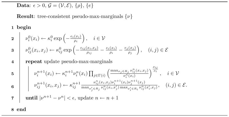
|
Appendix B. ILP formulation
The ILP formulation for the GMEC problem referred in this paper is as follows:
| (25) |
| (26) |
| (27) |
| (28) |
| (29) |
An LP relaxation can be obtained by simply dropping constraints (28)–(29). The resulting LP is equivalent to the tree-relaxed LP47.
Appendix C. Proof of Lemma 1
From (17), we have
| (30) |
Since ν is tree-consistent with every S ∈
, we can easily find a MAP assignment xS such that xS ∈ arg maxx
pS(x; ν) using dynamic programming50. Then, due to the assumption that ν is tree-consistent with S and is in a normal form, we have the following properties:
| (31) |
| (32) |
Therefore,
| (33) |
Since (33) is true for every S ∈
and ΣS∈
ρ(S) = 1, we obtain maxx
p(x) ≤ νc/Z from (30).
Appendix D. Proof of Lemma 2
From (17), we have
| (34) |
By the definition of max-marginals and the assumption that ν is tree-consistent, for S ∈
such that ζ ∈
(S), we have
| (35) |
for some constant κζ. We know there exists r* ∈ Rζ such that
| (36) |
Then, since ν is in a normal form, νζ(r*) = 1. We know from (33) in the proof of Lemma 1, that max{x|xζ= r*}pS(x; ν) = maxx pS(x; ν) = 1. Therefore, κζ = 1, and
| (37) |
On the other hand, for all S ∈
such that ζ ∉
(S), we know max{x|xζ= r}
pS(x; ν) = maxx
pS(x; ν) = 1. Plugging the obtained values of max{x|xζ = r}
pS(x; ν) and ΣS∈
:
ζ∈
(S)
ρ(S) = ρζ into (34), we obtain max{x|xζ = r}
p(x) ≤ (νc/Z)νζ(r)ρζ.
Appendix E. Proof of Lemma 3
If ζ, η ≠
(S), we know max{x|xζ=r, xη=spS(x; ν) = maxx
pS(x; ν). Then, since ν is tree-consistent and in a normal form, max{x|xζ=r,xη=s}pS(x; ν) = 1 from (33).If ζ ∈
(S), and η ∉
(S), we know max{x|xζ=r,xη=s}pS(x; ν) = max{x|xζ=r}pS(x; ν). Then, from (37), max{x|xζ=r,xη=s}pS(x; ν) = νζ(r)If (ζ, η) ∈
(S), by the definition of max-marginals and the assumption that ν is tree-consistent with every S, we have νζη(r, s) = κζηmax{x|(xζxη)=(r,s)}
pS(x; ν), for some constant κζη. We also know there exists (r*, s*) ∈ Rζ × Rη such that νζη(r*, s*) = max(xζ,xη)∈Rζ ×
Rη νζη(xζ, xη) = κζη max{x|(xζ,xη=(r*,s*)}
pS(x; ν). Then, since ν is in a normal form, i.e. νζη(r*, s*) = 1 and we have max{x|(xζxη)=(r*,s*)}
pS(x; ν) = maxx
pS(x; ν) = 1 from (33), we obtain κζη = 1. Therefore, max{x|(xζ,xη=(r,s)}
pS(x; ν) = νζη(r, s).- If ζ, η (S) and (η, ν) ∉
(S), let ξ = γ(S). Then,
(38) (39) (40) (41)
From the tree-consistency of ν, we have νξ(xξ) = βξj maxxj
νξj (xξ, xj) for some βξj > 0. We can also easily find xS such that xS ∈ arg maxx
pS(x; ν) using the tree-consistency of ν. Then, since ν is in a normal form, we have
, and
. Therefore, βξj = 1, and νξ (xξ) = maxxj
νξj (xξ, xj). So the maximization over xj in the parentheses of (41) is equal to 1 for all j ∈
(S)\{ζ, η,ξ}. Therefore,
References
- 1.Chothia C, Lesk AM. EMBO J. 1986;5(4):823–826. doi: 10.1002/j.1460-2075.1986.tb04288.x. [DOI] [PMC free article] [PubMed] [Google Scholar]
- 2.Ring CS, Cohen FE. FASEB J. 1993;7:783–790. doi: 10.1096/fasebj.7.9.8330685. [DOI] [PubMed] [Google Scholar]
- 3.Baker D, Sali A. Science. 2001;294(5540):93–96. doi: 10.1126/science.1065659. [DOI] [PubMed] [Google Scholar]
- 4.Drexler KE. Proc Natl Acad Sci USA. 1981;78:5275–5278. doi: 10.1073/pnas.78.9.5275. [DOI] [PMC free article] [PubMed] [Google Scholar]
- 5.Pabo C. Nature. 1983;301:200. doi: 10.1038/301200a0. [DOI] [PubMed] [Google Scholar]
- 6.Godzik A, Kolinski A, Skolnick J. J Comput Aided Mol Des. 1993;7(4):397–438. doi: 10.1007/BF02337559. [DOI] [PubMed] [Google Scholar]
- 7.Hellinga HW, Richards FM. Proc Natl Acad Sci USA. 1994;91:5803–5807. doi: 10.1073/pnas.91.13.5803. [DOI] [PMC free article] [PubMed] [Google Scholar]
- 8.Dahiyat BI, Mayo SL. Protein Sci. 1996;5:895–903. doi: 10.1002/pro.5560050511. [DOI] [PMC free article] [PubMed] [Google Scholar]
- 9.Kuhlman B, Dantas G, Ireton GC, Varani G, Stoddard BL, Baker D. Science. 2003;302:1364–1368. doi: 10.1126/science.1089427. [DOI] [PubMed] [Google Scholar]
- 10.Ponder JW, Richards FM. J Mol Biol. 1987;193(4):775–791. doi: 10.1016/0022-2836(87)90358-5. [DOI] [PubMed] [Google Scholar]
- 11.Dunbrack RL, Karplus M. J Mol Biol. 1993;230:543–574. doi: 10.1006/jmbi.1993.1170. [DOI] [PubMed] [Google Scholar]
- 12.Desmet J, De Maeyer M, Hazes B, Lasters I. Nature. 1992;356:539–542. doi: 10.1038/356539a0. [DOI] [PubMed] [Google Scholar]
- 13.Weiner SJ, Kollman PA, Case DA, Singh UC, Ghio C, Alagona G, Profeta S, Jr, Weiner P. J Am Chem Soc. 1984;106(3):765–784. [Google Scholar]
- 14.Weiner SJ, Kollman PA, Nguyen DT, Case DA. J Comput Chem. 1986;7(2):230–252. doi: 10.1002/jcc.540070216. [DOI] [PubMed] [Google Scholar]
- 15.Cornell WD, Cieplak P, Bayly CI, Gould IR, Merz KM, Jr, Ferguson DM, Spellmeyer DC, Fox T, Caldwell JW, Kollman PA. J Am Chem Soc. 1995;117:5179–5197. [Google Scholar]
- 16.Brooks BR, Bruccoleri RE, Olafson BD, States DJ, Swaminathan S, Karplus M. J Comput Chem. 1983;4:187–217. [Google Scholar]
- 17.Mackerell AD, Bashford D, Bellott M, Dunbrack RL, Evanseck JD, Field MJ, Fischer S, Gao J, Guo H, Ha S, Joseph-Mccarthy D, Kuchnir L, Kuczera K, Lau FTK, Mattos C, Michnick S, Ngo T, Nguyen DT, Prodhom B, Reiher WE, Roux B, Schlenkrich M, Smith JC, Stote R, Straub J, Watanabe M, Wiorkiewicz-Kuczera J, Yin D, Karplus M. J Phys Chem B. 1998;102:3586–3616. doi: 10.1021/jp973084f. [DOI] [PubMed] [Google Scholar]
- 18.Halgren TA. J Comput Chem. 1996;17:490–519. [Google Scholar]
- 19.Jorgensen WL, Tirado-Rives J. J Phys Chem. 1996;100(34):14508–14513. [Google Scholar]
- 20.Korte B, Vygen J. 2 Springer-Verlag; 2002. [Google Scholar]
- 21.Goldstein RF. Biophys J. 1994;66:1335–1340. doi: 10.1016/S0006-3495(94)80923-3. [DOI] [PMC free article] [PubMed] [Google Scholar]
- 22.Lasters I, De Maeyer M, Desmet J. Protein Eng. 1995;8:815–822. doi: 10.1093/protein/8.8.815. [DOI] [PubMed] [Google Scholar]
- 23.Gordon DB, Mayo SL. J Comput Chem. 1998;13:1505–1514. [Google Scholar]
- 24.Pierce NA, Spriet JA, Desmet J, Mayo SL. J Comput Chem. 2000;21:999–1009. [Google Scholar]
- 25.Looger LL, Hellinga HW. J Mol Biol. 2001;307:429–445. doi: 10.1006/jmbi.2000.4424. [DOI] [PubMed] [Google Scholar]
- 26.Gordon DB, Hom GK, Mayo SL, Pierce NA. J Comput Chem. 2003;24:232–243. doi: 10.1002/jcc.10121. [DOI] [PubMed] [Google Scholar]
- 27.Georgiev I, Lilien RH, Donald BR. Bioinformatics. 2006;22(14):174–183. doi: 10.1093/bioinformatics/btl220. [DOI] [PubMed] [Google Scholar]
- 28.Leach AR, Lemon AP. Proteins. 1998;33:227–239. doi: 10.1002/(sici)1097-0134(19981101)33:2<227::aid-prot7>3.0.co;2-f. [DOI] [PubMed] [Google Scholar]
- 29.Gordon DB, Mayo SL. Structure. 1999;7(9):1089–1098. doi: 10.1016/s0969-2126(99)80176-2. [DOI] [PubMed] [Google Scholar]
- 30.Wernisch L, Hery S, Wodak SJ. J Mol Biol. 2000;301:713–736. doi: 10.1006/jmbi.2000.3984. [DOI] [PubMed] [Google Scholar]
- 31.Eriksson O, Zhou Y, Elofsson A. Proceedings of WABI 2001, Vol. 2149 of LNCS; Springer; 2001. pp. 128–141. [Google Scholar]
- 32.Althaus E, Kohlbacher O, Lenhof HP, Müller P. J Comput Biol. 2002;9:597–612. doi: 10.1089/106652702760277336. [DOI] [PubMed] [Google Scholar]
- 33.Kingsford C, Chazelle B, Singh M. Bioinformatics. 2005;21(7):1028–1036. doi: 10.1093/bioinformatics/bti144. [DOI] [PubMed] [Google Scholar]
- 34.Leaver-Fay A, Kuhlman B, Snoeyink J. Pacific Symposium on Biocomputing. Vol. 10. World Scientific Publishing; 2005. pp. 16–27. [PubMed] [Google Scholar]
- 35.Xu J. Proceedings of RECOMB 2005; Springer; 2005. pp. 423–439. [Google Scholar]
- 36.Xie W, Sahinidis NV. Bioinformatics. 2006;22(2):188–194. doi: 10.1093/bioinformatics/bti763. [DOI] [PubMed] [Google Scholar]
- 37.Yanover C, Meltzer T, Weiss Y. J Mach Learn Res. 2006;7:1887–1907. [Google Scholar]
- 38.Weiss Y, Yanover C, Meltzer T. Proceedings of UAI 2007; 2007. [Google Scholar]
- 39.Desjarlais JR, Handel TM. J Mol Biol. 1999;289:305–318. doi: 10.1006/jmbi.1999.2866. [DOI] [PubMed] [Google Scholar]
- 40.Peterson RW, Dutton PL, Wand AJ. Protein Sci. 2004;13:735–751. doi: 10.1110/ps.03250104. [DOI] [PMC free article] [PubMed] [Google Scholar]
- 41.Koehl P, Delarue M. J Mol Biol. 1994;239:249–275. doi: 10.1006/jmbi.1994.1366. [DOI] [PubMed] [Google Scholar]
- 42.Desjarlais JR, Handel TM. Protein Sci. 1995;4:2006–2018. doi: 10.1002/pro.5560041006. [DOI] [PMC free article] [PubMed] [Google Scholar]
- 43.Jones DT. Protein Sci. 1994;3:567–574. doi: 10.1002/pro.5560030405. [DOI] [PMC free article] [PubMed] [Google Scholar]
- 44.Jiang X, Farid H, Pistor E, Farid R. Protein Sci. 2000;9:403–416. doi: 10.1110/ps.9.2.403. [DOI] [PMC free article] [PubMed] [Google Scholar]
- 45.Yanover C, Weiss Y. Proceedings of NIPS 2002; 2002. [Google Scholar]
- 46.Hart PE, Nilsson NJ, Raphael B. IEEE Trans Syst Sci Cyber. 1968;2:100–107. [Google Scholar]
- 47.Wainwright MJ, Jaakkola TS, Willsky AS. IEEE Trans Inform Theory. 2005;51(11):3697–3717. [Google Scholar]
- 48.Nemhauser GL, Wolsey LA. Integer and Combinatorial Optimization. Wiley; N. Y: 1988. [Google Scholar]
- 49.Cowell RG, Dawid AP, Lauritzen SL, Spiegehalter DJ. Probabilistic Networks and Expert Systems. Springer-Verlag; New York: 1999. [Google Scholar]
- 50.Wainwright MJ, Jaakkola T, Jordan MI. Stat Comput. 2004;14:143–166. [Google Scholar]
- 51.Kolmogorov V. IEEE Trans Pattern Anal. 2006;28:1568–1583. doi: 10.1109/TPAMI.2006.200. [DOI] [PubMed] [Google Scholar]
- 52.Hong E-J, Lozano-Pérez T. Proceedings of WABI 2006, Vol. 4175 of LNCS; Springer; 2006. pp. 219–230. [Google Scholar]
- 53.Altman MD. PhD thesis. Massachusetts Institute of Technology; Cambridge, MA, U.S.A: 2006. Computational ligand design and analysis in protein complexes using inverse methods, combinatorial search, and accurate solvation modeling. [Google Scholar]
- 54.Eckstein J, Phillips CA, Hart WE. Pico: an object oriented framework form parallel branch and bound. Technical report, RUTCOR. 2001 [Google Scholar]
- 55.Main AL, Harvey TS, Baron M, Boyd J, Campbell ID. Cell. 1992;71(4):671–678. doi: 10.1016/0092-8674(92)90600-h. [DOI] [PubMed] [Google Scholar]
- 56.Braden BC, Souchon H, Eisele JL, Bentley GA, Bhat TN, Navaza J, Poljak RJ. J Mol Biol. 1994;243(4):767–81. doi: 10.1016/0022-2836(94)90046-9. [DOI] [PubMed] [Google Scholar]
- 57.Bhat TN, Bentley GA, Boulot G, Greene MI, Tello D, Dallacqua W, Souchon H, Schwarz FP, Mariuzza RA, Poljak RJ. Proc Natl Acad Sci USA. 1994;91:1089–1093. doi: 10.1073/pnas.91.3.1089. [DOI] [PMC free article] [PubMed] [Google Scholar]
- 58.Syed R, Reid S, Li C, Cheetham J, Aoki K, Liu B, Zhan H, Osslund T, Chirino A, Zhang J, Finer-Moore J, Elliott S, Sitney K, Katz B, Matthews D, Wendoloski J, Egrie J, Stroud R. Nature. 1998;395:511–516. doi: 10.1038/26773. [DOI] [PubMed] [Google Scholar]
- 59.Dunbrack RL. Curr Opin Struct Biol. 2002;12(4):431–440. doi: 10.1016/s0959-440x(02)00344-5. [DOI] [PubMed] [Google Scholar]
- 60.Lippow SM, Wittrup KD, Tidor B. Nat Biotechnol. 2007;25:1171–1176. doi: 10.1038/nbt1336. [DOI] [PMC free article] [PubMed] [Google Scholar]