

Abstract
Intracellular microtubule polymerization dynamics are spatiotemporally controlled by numerous microtubule-associated proteins and other mechanisms, and this regulation is central to many cell processes. Here, we give an overview and practical guide on how to acquire and analyze time-lapse sequences of dynamic microtubules in live cells by either fluorescently labeling entire microtubules or by utilizing proteins that specifically associate only with growing microtubule ends, and summarize the strengths and weaknesses of different approaches. We give practical recommendations for imaging conditions, and we also discuss important limitations of such analysis that are dictated by the maximal achievable spatial and temporal sampling frequencies.
I. Introduction
Microtubules (MTs) are highly dynamic cytoskeletal polymers composed of α/β-tubulin dimers, and precise regulation of intracellular MT dynamics is important for many biological processes ranging from proper attachment and segregation of chromosomes during mitosis (Wittmann et al., 2001) to local stabilization of MTs toward the front of migrating cells (Wittmann and Waterman-Storer, 2001). MTs in cells and in vitro stochastically switch between phases of growth and shortening. This non-equilibrium polymerization behavior has been termed dynamic instability (Mitchison and Kirschner, 1984), and is driven by different structural states of the MT end, which are ultimately the result of polymerization-coupled GTP hydrolysis in the MT lattice (Fig. 1) (Nogales and Wang, 2006). GTP-loaded tubulin dimers initially polymerize as a relatively flat open sheet at the plus end of a growing MT, which subsequently closes into a tube. Shortly after polymerization GTP is hydrolyzed to GDP within the MT lattice, which is thought to leave a short GTP-tubulin cap at the tip of the MT. This remaining GTP-cap stabilizes the growing end and supports further addition of GTP-loaded tubulin subunits, resulting in a stable growth phase. In contrast, loss of the GTP-cap results in catastrophic depolymerization, and by electron microscopy highly curved protofilaments seem to peel away from the depolymerizing MT end. These frayed MT ends reflect the high intrinsic curvature of GDP-loaded tubulin dimers, and do not support addition of new GTP-loaded tubulin subunits. Thus, this large structural difference between polymerizing and depolymerizing MT ends is sufficient to explain the high persistency and abrupt switching between growing and shortening that characterizes MT dynamic instability in vitro (Kueh and Mitchison, 2009).
Figure 1. Diagram of different phases of MT polymerization dynamics.
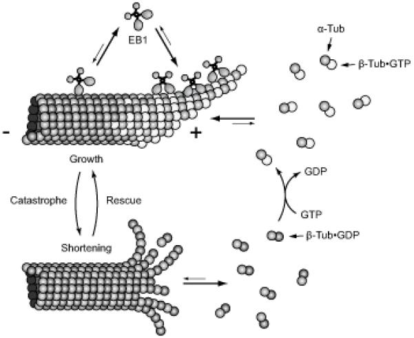
MT growth is thought to be accompanied by a protective cap of GTP-loaded tubulin at growing MT ends. The structurally distinct GTP-tubulin cap also provides a platform for the binding of MT plus end tracking proteins, +TIPs (Akhmanova and Steinmetz, 2008), that can be used as indirect reporters of intracellular MT polymerization dynamics.
Four parameters are generally measured to describe MT polymerization dynamics: the rates of growth (polymerization), shortening (depolymerization), and the transition frequencies between these two states. The transition from growth to shortening is referred to as ‘catastrophe’, and the transition from shortening to growth is referred to as ‘rescue’ (Fig. 1). These parameters can be determined quite easily in in vitro polymerization reactions with purified components because MT growth and shortening rates are relatively constant and transitions occur infrequently. In cells, however, MT polymerization dynamics are spatiotemporally highly regulated by a large number of accessory proteins (van der Vaart et al., 2009) as well as physical interactions with other intracellular structures (Dogterom et al., 2005). As a result intracellular MT polymerization dynamics are significantly more complex and more difficult to quantify. In vivo, only MT plus ends exhibit dynamic instability. Free minus ends are either stabilized or depolymerize. Both growth and shortening rates are highly variable, and rates of individual MTs fluctuate significantly over relatively short time periods. In addition, MT polymerization dynamics in cells often include relatively long periods of pause during which MT ends do not appear to grow or shorten within the resolution limit of the light microscope. Furthermore, intracellular MTs are subject to pulling and pushing forces, which result in MT buckling, breakage and movements of MT ends that are not due to polymerization dynamics (Brangwynne et al., 2007; Waterman-Storer and Salmon, 1997; Wittmann et al., 2003).
II. Rationale
The objective of this chapter is to give an overview of different techniques to observe and analyze intracellular MT dynamics either by continuous MT labeling or by the expression of fluorescently labeled proteins that specifically recognize growing MT ends. We aim to emphasize the strength and limitations of each approach, and discuss the theoretical boundaries of intracellular MT dynamics analysis that are imposed by the spatial and temporal resolution limits of light microscopy. Finally, it is important to note that these fundamental limitations similarly impact other intracellular tracking problems such as for example vesicular trafficking.
III. Imaging and Analysis of Homogeneously Labeled MTs
A. Probes to Visualize Dynamic MTs
Conventional analysis of intracellular MT dynamics involves homogenous labeling of the entire MT network. This was initially achieved by microinjection of tubulin in which surface amino groups that are exposed in polymerized MTs are chemically labeled using N-hydroxysuccinimide-derivatized fluorescent dyes (Sammak and Borisy, 1988; Shelden and Wadsworth, 1993). Several protocols are published describing tubulin labeling and microinjection procedures (Hyman et al., 1991; Waterman-Storer, 2002; Wittmann et al., 2004), and fluorescently labeled tubulin is also available commercially (e.g. from Cytoskeleton Inc.). Because microinjection is technically difficult, time-consuming, and only very few cells are available for analysis per experiment, this has mostly been replaced by the exogenous expression of tubulin tagged with fluorescent proteins (FPs). However, it should be noted that fluorescent dye-conjugated tubulin has some advantages over FP-tagged tubulin. Synthetic fluorescent dyes are generally brighter than FPs due to a higher extinction coefficient and better quantum yield, and because fluorescent dyes are small, dye-conjugated tubulin appears to be more efficiently incorporated into MTs. Together, this results in a higher MT to cytoplasm fluorescence ratio than FP-tagged tubulin. Finally, photobleaching of synthetic fluorophores is largely oxygen-dependent and can be efficiently inhibited by oxygen depletion from the tissue culture medium (Waterman-Storer, 2002; Wittmann et al., 2003; Wittmann et al., 2004).
Nevertheless, we and others have successfully used FP-tagged α- or β- tubulin to image and analyze intracellular MT polymerization dynamics (Rusan et al., 2001; Kumar et al., 2009). Although a growing toolbox of fluorescent proteins is now available, EGFP-tagged tubulin still appears to be the brightest and most photostable variant. For dual-color imaging we have also successfully used mCherry-tagged tubulin (Fig. 2 A). In addition, recent advances in elucidating the mechanisms of FP photobleaching indicate that FP photostability can be significantly improved by using riboflavin-free media (Bogdanov et al., 2009). Plasmid vectors suitable for transient transfections encoding different FP-tubulin fusion proteins are available from a variety of sources. We also routinely use adenovirus particles to transiently introduce FP-tagged tubulin and other cytoskeleton proteins into difficult to transfect cells (Kumar et al., 2009). However, because the correct folding of α/β tubulin dimers relies on a complex pathway involving several specific chaperones (Szymanski, 2002), care should be taken not to overwhelm the cells biosynthetic machinery by using too much virus. Too rapid expression of tagged tubulin results in poor incorporation into the MT cytoskeleton and excessive cytoplasmic background.
Figure 2. Semi-manual analysis of continuously labeled MTs.

(A) Images from a time-lapse sequence of mCherry-tagged tubulin. Images were acquired every 625 milliseconds (1.6 frames per second) for 1 minute. Scale bar, 5 μm. (B) Traces of the two MT ends indicated by arrowheads in A obtained by computer-assisted hand-clicking. (C) Life-history plots of MT #1 at the original time resolution, and at a simulated frame rate of 0.4 frames per second by only analyzing every 4th image. This demonstrates the averaging of the high variability of intracellular MT polymerization dynamics at slower frame rates.
While stable mammalian cell lines expressing FP-tubulins have been made and are viable (Rusan et al., 2001), it has so far not been possible to generate whole animals expressing FP-tagged tubulin, indicating that the FP-tag does disrupt developmentally important tubulin functions. In an alternative approach, mice expressing the MT-binding domain of a MT-associated protein, ensconsin, display homogeneously labeled MTs and are viable (Lechler and Fuchs, 2007). In addition, the MT signal can be increased by attaching up to five GFP moieties to ensconsin (Bulinski et al., 2001). Although GFP-ensconsin does not appear to modify intracellular MT dynamics, appropriate controls should be included when expressing exogenous MT-binding domains.
B. Preparation of Purified, Concentrated Adenovirus Particles
Although extensive adenovirus methods are published (Luo et al., 2007), we include a short reference protocol for the preparation of concentrated, purified adenovirus particles that we routinely use to prepare virus stock to introduce FP-tagged proteins in many different cell types. AdEasy-based viral genomes for the expression of EGFP-tubulin and EB1-EGFP from our lab are available through AddGene. Although these viruses are replication-deficient and new virus can only be produced in the packaging cell line, the experimentalist should be aware that these are infectious particles. At all times adhere to the required BSL-2 safety precautions, and sterilize and dispose infectious material according to the appropriate local regulations.
Required materials
PacI-linearized and purified AdEasy viral plasmid containing the gene of interest
Transfection reagent (e.g. Lipofectamine 2000, Invitrogen Cat. No. 11668-027)
Adenovirus packaging cell line (AD-293, Stratagene)
Dulbecco’s Modified Eagle Medium (DMEM, Invitrogen Cat. No. 10313) supplemented with 10% Fetal Bovine Serum (FBS, Invitrogen Cat. No. 26140), 10 mM MgCl2, 2 mM L-glutamine (Invitrogen Cat. No. 25030), 1x Penicillin/Streptomycin (Invitrogen Cat. No. 15140)
10 mM Tris-Cl pH 8.0
Low density CsCl buffer (ρ = 1.2 g/ml): Dissolve 35 g CsCl in a final volume of 100 ml 10 mM Tris-Cl pH 8.0
High density CsCl buffer (ρ = 1.45 g/ml): Dissolve 53 g CsCl in a final volume of 100 ml 10 mM Tris-Cl pH 8.0
ARCA buffer: 10 mM Tris-Cl, pH 8.0, 1 mM MgCl2, 5% sucrose, 1% glycine,
0.05% Tween-80
Beckman ultracentrifuge and tubes: 38.5 ml (Beckman Cat. No. 41103909 for SW 28 Ti rotor) and 13.2 ml (Beckman Cat. No. 41103909 for SW 41 Ti rotor)
Econo-Pac 10DG Desalting Columns (Bio-Rad Laboratories Cat. No. 732-2010)
Adenovirus production and amplification
Transfect a 6 cm dish of ~50% confluent AD-293 cells with the linearized AdEasy viral genome according to the manufacturer’s instructions in antibiotic-free DMEM. We commonly use Lipofectamine 2000. AD-293 cells do not adhere well to tissue culture plastic and care should be taken not to disrupt the monolayer after transfection.
Grow transfected cells until the cytopathic effect (CPE) of virus production becomes visible. At this point, cells start to round up and lift off from the bottom of the plate. Depending on transfection efficiency, this will take approximately 1-2 weeks. Gently change medium when it turns too acidic without disrupting the cell monolayer. Transfection efficiency can also be estimated by fluorescence microscopy because transfected cells will express the EGFP-tagged fusion protein.
Harvest all cells and media by gently tapping the plate and pipetting up and down into a 15-ml centrifuge tube. Centrifuge at 4°C, 1200 rpm, 5 minutes. Discard supernatant and resuspend pellet in 1 ml sterile 10 mM Tris-Cl pH 8.0.
Lyse cells by freezing for 5-10 min in a dry ice/EtOH bath, then thaw completely in a 37°C water bath. Repeat freeze/thaw cycle three times. Centrifuge to remove cell debris at 4000 rpm for 20 min, 4°C. The supernatant now contains first generation virus, which is used for all subsequent amplifications. Remove 200 μl for the next step and freeze the rest at −80°C.
For subsequent virus amplification, infect a 10 cm dish of ~80% confluent AD-293 cells: Remove medium from cells, and gently add 200 μl of the first generation virus diluted to 2 ml in DMEM. After 1 hour add additional 8 ml DMEM. Harvest cells as in Step 3 as soon as CPE becomes evident.
Repeat the infection and amplification cycle (Step 3-5) until CPE is visible within 48 hours post-infection. This should take a total of 2-3 cycles.
Large-scale adenovirus production
7. Prepare twenty large plates (15 cm diameter or similar) of AD-293 cells. To ensure that cells are plated evenly, prepare cell suspension in a media bottle, mix, and plate 20 ml into each dish. At this point, DMEM with 5% FBS can be used to conserve serum.
8. Grow cells to ~90% confluency. Dilute 0.5 ml virus from Step 6 into 100 ml DMEM. Infect each plate with 5 ml of the diluted virus, mix gently, and return plates to incubator. After 48 hours the virus-induced CPE should be clearly visible.
9. Harvest the cells and medium by pipetting up and down or by using a cell scraper. Centrifuge at 1200 rpm, 10 min, 4°C. Discard supernatant and resuspend pellet in 13 ml of 10 mM Tris-CL pH 8.0.
10. Lyse cells with three freeze/thaw cycles (as in Step 4), and vortex for 30 seconds after each thaw. Centrifuge at 4000 rpm, 20 min, 4°C. Collect and keep supernatant on ice. It is very important for the subsequent purification step that all cell debris is removed.
Adenovirus purification by cesium chloride density gradient centrifugation
11. Prepare two CsCl step gradients in 38.5-ml Beckman Ultraclear centrifuge tubes: First, slowly pour 10 mL of low density CsCl buffer into centrifuge tube. Then gently underlay 10 mL of high density CsCl by carefully inserting and pipetting to the bottom of the tube. Gently overlay virus supernatant on top of the step gradient. Fill tube completely with 10 mM Tris pH 8.0 to avoid collapse during ultracentrifugation. The second CsCl gradient tube is filled with 10 mM Tris pH 8.0 and used as balance. Make sure the tubes are well balanced, and that everything is kept sterile in a BSL-2 laminar flow tissue culture hood.
12. Centrifuge at 20,000 rpm in an SW 28 Ti swinging bucket rotor with slow acceleration and no brakes, for 2 hours at 4°C. Unload tubes in tissue culture hood, and place tube in ring stand near eye level. A bluish band about halfway down the tube contains purified, concentrated virus. Just above there is usually a second, fainter band containing defective virus particles. During extraction of the virus band, care should be taken to avoid contamination from this upper band.
13. Remove some of the excess liquid from above the virus, being extremely careful not to disturb the band. Wipe the outside of the tube with ethanol to sterilize. Stick a piece of adhesive tape on the side of the tube where it is to be punctured to avoid leakage. Carefully pierce the tube with a hypodermic syringe with an 18 gauge needle slightly below the bluish virus band. Be sure to use as little force as possible in order not to pierce through both sides of the tube. Remember that the band contains highly concentrated virus particles. Thus, keep hands out of the way, and make sure to wear appropriate personal protective equipment. Tilt the needle upward into the virus band and draw approximately 3 ml of the virus slowly into the syringe. Leave the syringe with needle in the tube, and pipet liquid from the tube until it is below the needle. Now remove the syringe and expel the virus into a sterile 15-ml polypropylene tube.
14. Dilute virus to 4 ml with 10 mM Tris pH 8.0. This is essential to reduce the density to below 1.2 g/ml. Prepare a smaller step gradient with 4 ml of each CsCl buffer as in Step 11, but in smaller 13.2-ml tubes. Overlay with the diluted virus and fill tube with 10 mM Tris pH 8.0. Centrifuge at 20,000 rpm at 4°C in an SW 41 Ti rotor, and isolate virus band as in Step 13.
15. Desalt virus on a 10DG column: Equilibrate column with 30 ml ARCA buffer. Load 3 ml of the virus, and collect 0.5 ml fractions on ice. Concentrated virus should start eluting in the third fraction. Concentrated, opaque fractions can be pooled, aliquoted, and stored at −80°C. This procedure yields highly infectious adenovirus particles, and we generally use less than 1 μl adenovirus stock to infect cells for microscopy. Virus titer can be estimated by measuring optical density at 260 nm in PBS containing 1% SDS (1OD ~ 1.1 × 10¹² virus particles per ml).
C. Imaging of Intracellullar MT Dynamics
Analysis of intracellular MT dynamics relies on time-lapse imaging of fluorescently labeled proteins. Different modalities of fluorescence microscopy including widefield epifluorescence, confocal and total internal reflection (TIRF) microscopy can and have been used to image MT dynamics although each has its limitations. In widefield images, out-of-focus blur severely limits the ability to observe MTs in thicker cell regions and only works reasonably well in flat, peripheral cell areas (Wittmann et al., 2003). Although TIRF microscopy produces superior contrast, it only allows imaging of MTs in very close proximity of the bottom cell membrane (Krylyshkina et al., 2003) [Akhmanova chapter this book]. We mostly use spinning disk confocal microscopy as a versatile method to image dynamic MTs because it combines thin optical sectioning, which largely eliminates out-of-focus blur, with better sample penetration compared with TIRF.
Independent of the exact microscopy modality used, it is important to acquire images at the best possible spatial resolution. At the emission wavelength of EGFP of about 510 nm, the resolution limit of a fluorescence light microscope with a 1.4 NA objective lens under optimal conditions is ~250 nm. Because tubulin dimers are about 8 nm long and are thus small compared to this approximate diameter of the microscope point spread function, any discernible MT length change represents the addition or removal of several hundred tubulin subunits. In order to be able to image changes as close to the molecular scale as possible, it is important that the digital camera used to acquire images is of sufficiently high resolution to oversample the optical resolution to fulfill the Nyquist sampling criterion (Wittmann et al., 2004). This means that the effective pixel size of the captured image should be ~2-3 fold smaller than the resolution limit. On a microscope system with no intermediate magnification this can be achieved with a 60x or 100x objective and a high-resolution scientific grade charge-coupled device (CCD) camera. Such cameras from different manufacturers typically use a Sony Interline CCD sensor with 6.45 × 6.45 μm pixels resulting in an effective pixel size of ~107 nm in object space at 60x magnification. Electron multiplying CCD (EMCCD) cameras have much larger pixels up to 16 × 16 μm (effective pixel size of 266 nm at 60x), which is insufficient for optimal sampling of the optical resolution without additional magnification1. For similar reasons, the use of two-photon microscopy (which halves the optical resolution) or binning (which halves the detector resolution) is not optimal for MT dynamics imaging. Finally, it is important to remember that optimized imaging conditions are only achieved when cells are grown in two dimensions preferably on #1.5 cover glasses. We typically use glass-bottom tissue culture dishes (e.g. from MatTek Corporation), or custom-made sealed cover glass chambers (Wittmann et al., 2004). The imaging system should also be environmentally controlled because, as any biochemical reaction, the rate of microtubule polymerization is temperature-dependent. Imaging at high resolution becomes significantly more challenging for more physiological, three-dimensional samples.
Our lab uses a Yokogawa CSU-10 spinning disk confocal head with 200 mW 488 nm and 561 nm solid-state lasers in an LMM5 laser launch (Spectral Applied Research). In combination with 60x or 100× 1.49 NA TIRF objective lenses (Nikon) and a high-resolution CoolSNAP cooled CCD camera (Photometrics),we can achieve the highest spatial resolution possible with conventional light microscopy. Image acquisition is controlled by Nikon NIS-Elements software. With this setup we have been able to achieve frame rates of up to 4 frames per second at below 200 ms exposure times, although as outlined below manual tracking of continuously labeled MTs becomes highly error-prone at time intervals shorter than 2 to 5 seconds between frames. Thus, slightly longer exposure times (~500 ms) combined with lower illumination intensities are usually acceptable.
Because MT polymerization dynamics analysis requires long time-lapse sequences, it is crucial to minimize sample exposure and photodamage. There are relatively simple aspects in the design of an imaging system that are often overlooked, but significantly improve the performance of fluorescent live-cell microscopy. Excitation shutters should be hardware-controlled and triggered directly from the camera so that shutters are only open when an image is actually acquired. In contrast, software shutter control typically adds several hundred milliseconds of sample exposure before and after image acquisition, which results in significantly faster photobleaching especially at low exposure times. In addition, it is important to use optimized emission filter sets. For example, for single-channel EGFP imaging, we use a long-pass dichroic mirror and emission filter (Semrock) with edge wavelengths of ~500 nm. This allows maximum detection over most of the EGFP emission spectrum, and results in a greater than 50% signal increase at the same exposure settings compared to high quality multi-band pass filter sets.
D. Semi-manual Tracking and Analysis of Dynamic MTs
Accurate, automatic detection of the ends of continuously labeled MTs is a highly challenging computational problem. Although substantial progress is being made to develop computer vision algorithms to detect and track movement of continuously labeled MTs (Altinok et al., 2007; Hadjidemetriou et al., 2008) [Rose chapter this book], a robust solution is not currently available. However, computer-assisted hand-tracking in which the user manually selects MT ends in a time-lapse sequence can be done with a variety of available software packages (Fig. 2 B). We now mostly use the tracking function in NIS-Elements (Nikon), but similar functions are available in other image analysis software packages including MetaMorph (Molecular Dynamics) and ImageJ.
The output of such semi-manual tracking is a list of positions or displacements of the MT end as a function of time. It is important to remember that this list does not include information on whether an end displacement represents MT growth or shortening, and after the initial tracking we go through the list a second time to designate shortening events by negative numbers. MT end displacement can then be plotted (Fig. 2 C), and analyzed in different ways to calculate growth and shortening rates, transition frequencies, and the percent time MTs spend in growth, shortening, or pause phases. Because of the large variations of intracellular MT growth rates, we find it difficult to a priori designate phases of constant growth or shortening velocities in such life-history plots (Walker et al., 1988). Instead, we calculate instantaneous growth and shortening rates on a frame-to-frame basis. Because of the positional uncertainty introduced by image formation in the microscope and the error introduced by hand-clicking on the image, we then set a lower threshold of MT end displacement in the range of the optical resolution (Kumar et al., 2009; Wittmann et al., 2003). Growth or shortening events below this threshold are classified as a pause.
A drawback of this method is that the positional error becomes dominant if sequences are analyzed that are acquired at very short time intervals, which results in completely different measurements of microtubule dynamics parameters depending on the frame rate. In the example in Fig. 2, images were acquired at 1.6 frames per second (625 ms between images). Assuming a localization error of 1 pixel, which is about half the diameter of the point spread function and probably an overestimation of hand-clicking accuracy, any growth or shortening event below 10 μm/min is classified as a pause, overestimating the time MTs spend in a pause state (Fig. 3 A). This also truncates the lower end of the true growth and shortening rate populations, and results in a gross overestimation of the average rates (Fig. 3 B). At lower frame rates, this threshold becomes much more reasonable, and the measured growth and shortening rates better approach true intracellular rates. Nevertheless, because of this positional detection limit, slow MT polymerization events cannot be distinguished from bona fide pauses during which no polymerization or depolymerization occurs. Thus, the threshold below which an event is considered a pause is relatively arbitrary and largely depends on the imaging conditions.
Figure 3. Dependence of MT polymerization dynamics quantification on temporal resolution.
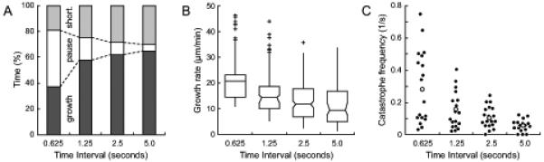
(A) Time MTs spend in different phases, (B) Growth rates, and (C) Catastrophe frequencies as a function of frame rate. 19 MTs from the sequence in Fig. 2 were analyzed, and simulated frame rates were obtained by temporal sub-sampling.
Transition frequencies are defined as follows: The catastrophe frequency is the number of transitions from growth to shortening divided by the time MTs spend growing. This is mathematically identical to the inverse of the average time MTs spend in an uninterrupted growth phase. Because true pauses cannot be clearly defined, we allow growth phases preceding a catastrophe to be interrupted by apparent pauses. Importantly, because events that occur between two acquired images are not observable, the imaging frame rate also defines an upper boundary for transition frequencies, and faster frame rates will result in the measurement of higher transition frequencies (Fig. 3 C). For example, at a slower time resolution of 0.2 frames per second (i.e. an image acquired every 5 seconds), the shortest observable growth interval is 5 seconds. Thus, the maximal observable catastrophe frequency is identical to the frame rate. Similarly, pauses shorter than 5 seconds cannot be observed contributing to the apparent increase in the time MTs spend in growth at lower frame rates (Fig. 3 A). Likewise, the rescue frequency is defined as the number of transitions from shortening to growth divided by the time MTs spend shortening, and the same limitations as for catastrophe frequencies apply.
In conclusion, because of the inevitable MT end localization error semi-manual analysis of MT dynamics is best performed on time-lapse sequences with images acquired every 2-5 seconds at high spatial resolution, which represents the range of frame rates used most frequently in published analysis of MT dynamics. These conditions are a good compromise to minimize the error introduced by positional inaccuracy, while still maintaining a relatively high time resolution for the quantification of transition frequencies. However, one should be aware of the inherent limitations of this analysis, and it is imperative to only compare quantifications obtained from time-lapse sequences acquired at identical magnification and frame rate (Shelden and Wadsworth, 1993). In addition, because semi-manual tracking is extremely time-consuming, the number of MTs analyzed is often low and it is challenging to obtain statistically sufficiently large data sets. Nevertheless, growth and shortening rates can be determined with good accuracy. Relatively large standard deviations on rate measurements reflect the variability of intracellular MT polymerization dynamics rather than measurement errors. In contrast, the number of observed catastrophes or rescues tends to be low, and care should be taken in interpreting differences in transition frequencies in different conditions. For any meaningful quantification, we would recommend to track 5-10 MTs per cell in at least five cells, and an observation time of around 5-10 minutes per MT.
IV. MT Fluorescent Speckle Microscopy
In time-lapse sequences of continuously labeled MTs it is not possible to distinguish between MT polymerization dynamics and MT translocation. However, fluorescent speckle microscopy (FSM) can be used to test whether MT end displacements are due to movements of the entire MT. The principle underlying MT FSM is simple and relies on the stochastic incorporation of fluorescently labeled tubulin subunits along the MT. At low intracellular ratios of fluorescently labeled to unlabeled tubulin, convolution with the microscope’s point spread function results in intensity variations (fluorescent speckles) along the MT (Waterman-Storer and Salmon, 1998; Wittmann et al., 2004). Although best speckle contrast is achieved at labeling ratios of below 1% labeled tubulin, intensity variations along MTs can be observed at much higher labeling ratios and are often evident in cells expressing low to moderate levels of FP-tagged tubulin. Simple image processing such as low pass filtering to remove camera pixel noise, and sharpening with an unsharp mask filter can be used to greatly increase speckle contrast (Wittmann et al., 2004). Because MTs only exchange subunits at the ends, the pattern of intensity variations along the MT is stable and can be used as a direct read-out for MT translocation (Fig. 4).
Figure 4. MT fluorescent speckle microscopy.

Montage of a time-lapse sequence of a MT fragment in a cell expressing constitutively active Rac1 (Wittmann et al., 2003) injected with X-rhodamine-labeled tubulin. One bright speckle is followed over time and highlighted by the dashed line. The speckle pattern reveals different types of MT movement that would be misinterpreted as polymerization dynamics if the MT were homogenously labeled. For example, in the second half of the sequence, the MT plus end remains in close contact with the cell edge and is apparently stationary. However, the appearance of new speckles is evidence for polymerization at the plus end and translocation of the speckle pattern demonstrates movement of the MT polymer.
V. Imaging and Analysis of Growing MT Ends
A. Probes to Visualize Growing MT Ends
Analysis of MT dynamics in time-lapse sequences of continuously labeled MTs suffers from a fundamental limitation. Even in cell areas in which MTs are only moderately dense, it quickly becomes impossible to clearly observe growing ends. Thus, conventional analysis of intracellular MT dynamics is subjective and regionally biased because it is limited to a small subpopulation of MTs near the cell periphery, where MT ends can be observed clearly over sufficient periods of time (Wittmann et al., 2003).
An alternative strategy to visualize intracellular MT dynamics utilizes fluorescently tagged proteins that specifically recognize growing MT plus ends (Akhmanova and Steinmetz, 2008; Salaycik et al., 2005). Because these proteins, commonly referred to as +TIPs, bind only weakly along MTs, growing MT ends are clearly visible in more central cell areas in which MTs are too dense to visualize MT ends directly (compare images of the same cell in Fig. 2 A and Fig. 5 A). End Binding Proteins, EBs, are the +TIP prototype and are thought to directly recognize the structurally distinct GTP-tubulin cap at growing MT ends (Fig. 1). EBs are small dimeric proteins containing an N-terminal MT-binding domain, and a C-terminal cargo-binding domain, and most if not all other +TIPs associate with growing MT ends through interactions with this C-terminal domain (Akhmanova and Steinmetz, 2008; Bieling et al., 2008; Honnappa et al., 2009). Because N-terminal FP-tags interfere with EB localization to MT ends (Skube et al., 2009), C-terminally tagged EB1- or EB3-EGFP constructs have been predominantly used to highlight growing MT ends in cells. The exponential decay of available binding sites results in the characteristic comet-like fluorescence profiles of EGFP-tagged EBs on MT ends. In addition, rapid binding kinetics of EBs (Dragestein et al., 2008) causes rapid loss of EB fluorescence from non-polymerizing MT ends, and rapid appearance of EB comets when MTs start growing. However, because EBs are central adaptor proteins that recruit many other +TIPs to growing MT ends, concerns have grown that EB-EGFP constructs may disrupt endogenous localization of other +TIPs and thus alter MT polymerization dynamics and cell behavior (Skube et al., 2009). Nevertheless, low level EB-EGFP expression appears relatively benign and we and others have made multiple stable EB1-EGFP-expressing cell lines that appear to behave normally. Similar to FP-tagged tubulin we also use adenovirus to introduce EB1-EGFP into difficult to transfect cells. One way to increase EB-EGFP signal at growing MT ends without increasing the overall expression level and background along MTs is to add multiple EGFP tags. Alternatively, EB-binding domains of other +TIPs such as CLIP-170 or CLASPs can be used to visualize intracellular MT polymerization dynamics (Komarova et al., 2009; Kumar et al., 2009; Wittmann and Waterman-Storer, 2005). Thus, different types of +TIPs can be used to validate experimental results and help eliminate potential +TIP overexpression-induced artifacts. Most importantly, a minimal EB-binding motif has recently been identified that is sufficient for plus end localization (Honnappa et al., 2009). It should therefore be possible to engineer artificial +TIPs that only minimally interfere with intracellular MT dynamics. The same considerations about high-resolution fluorescent live cell imaging as outlined in section II.C also apply for FP-tagged +TIPs.
Figure 5. +TIPs as reporters of MT polymerization dynamics.

(A) Images of EGFP-tagged EB1 from the same dual-wavelengths time-lapse sequence as in Fig. 2. Scale bar, 5 um. (B) Computer-generated growth tracks of the same two MTs as in Fig. 2 with shortening events (light grey arrows) inferred by geometrical cluster analysis. (C) Maximum intensity projection of the entire image sequence directly showing EB1-EGFP growth tracks. (D) Computer-generated growth tracks with a minimum life-time of four frames demonstrating high tracking fidelity.
B. Computational Tracking and Analysis of +TIP Dynamics
Because +TIPs specifically associate with growing MT ends, it is straight forward to determine growth rates from time-lapse sequences of FP-tagged +TIPs. For example, computer-assisted hand-tracking as described above for continuously labeled MTs can be used. Alternatively, maximum intensity projections of +TIP comet time-lapse sequences can be used to calculate growth rates directly from the comet-to-comet distance (Wittmann and Waterman-Storer, 2005). However, one immediately obvious challenge in using +TIPs to analyze MT polymerization dynamics is that MT ends are not visible during pause and shortening phases. Thus, only growth rates can be measured directly. To extract additional parameters of MT dynamic instability, a computational framework has recently been developed that breaks down the analysis of +TIP time-lapse sequences into three steps (Matov et al., 2010): First, a band-pass filter is used to detect objects of the size scale of +TIP comets. Second, these objects are tracked by single particle tracking. Such automated tracking is highly accurate (Fig. 5 C and D), and yields statistically large populations of MT growth rates (Jaqaman et al., 2008). For example, over 400 individual EB1-EGFP growth tracks were detected in the one minute sequence shown in Fig. 5. To eliminate tracks that result from detection errors, we generally only consider tracks for further analysis that have a life-time of at least 4 frames. In order to achieve good EB1-EGFP comet correspondence between subsequent frames and minimize the number of tracking errors, computational tracking approaches generally require higher frame rates (~1-2 frames per second) as compared to manual analysis. We have successfully used this approach to demonstrate spatial gradients of MT polymerization dynamics in migrating cells (Kumar et al., 2009).
Finally, +TIP growth tracks are linked by geometrical cluster analysis. This analysis relies on a priori knowledge of the physical characteristics and behavior of MTs. Intracellular MTs are laterally relatively immobile, and are stiff and bend very little over the short time window used to record +TIP dynamics. As a result, MT shortening, rescues and pauses predominantly occur in very close proximity to the path defined earlier by the growing end of the same MT (Fig. 2 B). A global combinatorial optimization algorithm that utilizes a cost function based on geometrical and temporal constraints between the beginning and the end of +TIP growth tracks can be used to determine those tracks that most likely belong to the same MT (Matov et al., 2010). Because of the statistical nature of this algorithm, it will make errors and clearly has some fundamental limitations. For example, terminal shortening phases are hidden because a shortening phase has to be followed by a growth phase in order to be detected by the clustering algorithm. In addition, to minimize the number of clustering errors, the constraints for linking individual growth tracks have to be kept quite stringent only allowing the search for a rescue event ~10-20 frames in the future. Thus, long shortening phases such as the one in MT #2 are frequently missed by the algorithm (compare Fig. 2 B and Fig. 5 B). Finally, growth phases are missed by the tracking algorithm if they are too slow and too short to produce a sufficient +TIP signal such as the short growth phases at the end of MT #1.
Thus, data derived by geometrical clustering of +TIP growth tracks cannot be directly compared to conventionally determined MT dynamics parameters. Nevertheless, because statistically large MT numbers can be analyzed relatively quickly using this approach, we expect this algorithm to be extremely useful to compare different experimental conditions on a relative basis. plusTipTracker, a Matlab-based open source software package enabling +TIP comet detection, growth track reconstruction, visualization, sub-cellular regional analysis, and MT subpopulation analysis will soon be available from http://lccb.hms.harvard.edu (Applegate et al., 2010).
VI. Conclusion
Because spatiotemporal regulation of intracellular MT dynamics is important in many aspects of cell biology, the interest in generally applicable methods for quantitative analysis of MT dynamics is high. In this chapter, we give a brief overview and practical guide on how to acquire and analyze time-lapse sequences of dynamic MTs in cells by either fluorescently labeling entire MTs or by utilizing proteins that specifically associate only with growing MT ends. Because of the optical resolution limit it is not possible to measure the ‘true’ position of a MT end with conventional light microscopy. Therefore, quantification of intracellular microtubule polymerization dynamics depends to a very large extent on the imaging conditions, sampling frequencies and analysis methods used, which define theoretical limits of rates and transition frequencies that can be determined from a particular data set. Thus, absolute MT dynamics parameters are only of very limited value, and measurements should only be used to compare different experimental conditions for which time-lapse sequences were recorded identically. It will be exciting to see if and how modern super-resolution techniques will be used to more precisely observe MT polymerization dynamics in cells. In addition, because of the structural and biochemical processes, and nanoscale fluctuations of polymerization dynamics that occur on MT plus ends (Schek, III et al., 2007; Kerssemakers et al., 2006), the conventional definition of MT growth and shortening rates and transition frequencies is most likely not sufficient to accurately capture the complexity of MT polymerization dynamics. This problem is further aggravated in cells, where MT polymerization dynamics are even more variable as a result of regulation by associated proteins. Novel methods to analyze MT dynamics are needed, and we provide an outlook on one such method that utilizes computational clustering of MT growth tracks defined by the association of fluorescently labeled +TIPs with growing MT ends. It will be interesting to see how such new computational approaches will impact our future understanding of intracellular MT function and dynamics.
Acknowledgements
S.G. is the recipient of an NSF graduate student fellowship. T.W. is supported by National Institutes of Health grant R01 GM079139. This research was in part conducted in a facility constructed with support from the Research Facilities Improvement Program grant C06 RR16490 from the National Center for Research Resources of the National Institutes of Health.
Footnotes
Up-to-date information and excellent tutorials about many aspects of light microscopy can also be found online, for example at www.microscopyu.com.
References
- Akhmanova A, Steinmetz MO. Tracking the ends: a dynamic protein network controls the fate of microtubule tips. Nat. Rev. Mol. Cell Biol. 2008;9:309–322. doi: 10.1038/nrm2369. [DOI] [PubMed] [Google Scholar]
- Altinok A, Kiris E, Peck AJ, Feinstein SC, Wilson L, Manjunath BS, Rose K. Model based dynamics analysis in live cell microtubule images. BMC. Cell Biol. 2007;8(Suppl 1):S4. doi: 10.1186/1471-2121-8-S1-S4. [DOI] [PMC free article] [PubMed] [Google Scholar]
- Applegate KT, Matov A, Jaqaman K, Danuser G. plusTipTracker: quantitative image analysis software for the measurement of microtubule dynamics. Mol. Biol. Cell. 2010 doi: 10.1016/j.jsb.2011.07.009. submitted. [DOI] [PMC free article] [PubMed] [Google Scholar]
- Bieling P, Kandels-Lewis S, Telley IA, van DJ, Janke C, Surrey T. CLIP-170 tracks growing microtubule ends by dynamically recognizing composite EB1/tubulin-binding sites. J. Cell Biol. 2008;183:1223–1233. doi: 10.1083/jcb.200809190. [DOI] [PMC free article] [PubMed] [Google Scholar]
- Bogdanov AM, Bogdanova EA, Chudakov DM, Gorodnicheva TV, Lukyanov S, Lukyanov KA. Cell culture medium affects GFP photostability: a solution. Nat. Methods. 2009;6:859–860. doi: 10.1038/nmeth1209-859. [DOI] [PubMed] [Google Scholar]
- Brangwynne CP, MacKintosh FC, Weitz DA. Force fluctuations and polymerization dynamics of intracellular microtubules. Proc. Natl. Acad. Sci. U. S. A. 2007;104:16128–16133. doi: 10.1073/pnas.0703094104. [DOI] [PMC free article] [PubMed] [Google Scholar]
- Bulinski JC, Odde DJ, Howell BJ, Salmon ED, Waterman-Storer CM. Rapid dynamics of the microtubule binding of ensconsin in vivo. J. Cell Sci. 2001;114:3885–3897. doi: 10.1242/jcs.114.21.3885. [DOI] [PubMed] [Google Scholar]
- Dogterom M, Kerssemakers JW, Romet-Lemonne G, Janson ME. Force generation by dynamic microtubules. Curr. Opin. Cell Biol. 2005;17:67–74. doi: 10.1016/j.ceb.2004.12.011. [DOI] [PubMed] [Google Scholar]
- Dragestein KA, van Cappellen WA, van HJ, Tsibidis GD, Akhmanova A, Knoch TA, Grosveld F, Galjart N. Dynamic behavior of GFP-CLIP-170 reveals fast protein turnover on microtubule plus ends. J. Cell Biol. 2008;180:729–737. doi: 10.1083/jcb.200707203. [DOI] [PMC free article] [PubMed] [Google Scholar]
- Hadjidemetriou S, Toomre D, Duncan J. Motion tracking of the outer tips of microtubules. Med. Image Anal. 2008;12:689–702. doi: 10.1016/j.media.2008.04.004. [DOI] [PubMed] [Google Scholar]
- Honnappa S, Gouveia SM, Weisbrich A, Damberger FF, Bhavesh NS, Jawhari H, Grigoriev I, van Rijssel FJ, Buey RM, Lawera A, Jelesarov I, Winkler FK, Wuthrich K, Akhmanova A, Steinmetz MO. An EB1-binding motif acts as a microtubule tip localization signal. Cell. 2009;138:366–376. doi: 10.1016/j.cell.2009.04.065. [DOI] [PubMed] [Google Scholar]
- Hyman A, Drechsel D, Kellogg D, Salser S, Sawin K, Steffen P, Wordeman L, Mitchison T. Preparation of modified tubulins. Methods Enzymol. 1991;196:478–485. doi: 10.1016/0076-6879(91)96041-o. [DOI] [PubMed] [Google Scholar]
- Jaqaman K, Loerke D, Mettlen M, Kuwata H, Grinstein S, Schmid SL, Danuser G. Robust single-particle tracking in live-cell time-lapse sequences. Nat. Methods. 2008;5:695–702. doi: 10.1038/nmeth.1237. [DOI] [PMC free article] [PubMed] [Google Scholar]
- Kerssemakers JW, Munteanu EL, Laan L, Noetzel TL, Janson ME, Dogterom M. Assembly dynamics of microtubules at molecular resolution. Nature. 2006;442:709–712. doi: 10.1038/nature04928. [DOI] [PubMed] [Google Scholar]
- Komarova Y, De Groot CO, Grigoriev I, Gouveia SM, Munteanu EL, Schober JM, Honnappa S, Buey RM, Hoogenraad CC, Dogterom M, Borisy GG, Steinmetz MO, Akhmanova A. Mammalian end binding proteins control persistent microtubule growth. J. Cell Biol. 2009;184:691–706. doi: 10.1083/jcb.200807179. [DOI] [PMC free article] [PubMed] [Google Scholar]
- Krylyshkina O, Anderson KI, Kaverina I, Upmann I, Manstein DJ, Small JV, Toomre DK. Nanometer targeting of microtubules to focal adhesions. J. Cell Biol. 2003;161:853–859. doi: 10.1083/jcb.200301102. [DOI] [PMC free article] [PubMed] [Google Scholar]
- Kueh HY, Mitchison TJ. Structural plasticity in actin and tubulin polymer dynamics. Science. 2009;325:960–963. doi: 10.1126/science.1168823. [DOI] [PMC free article] [PubMed] [Google Scholar]
- Kumar P, Lyle KS, Gierke S, Matov A, Danuser G, Wittmann T. GSK3beta phosphorylation modulates CLASP-microtubule association and lamella microtubule attachment. J. Cell Biol. 2009;184:895–908. doi: 10.1083/jcb.200901042. [DOI] [PMC free article] [PubMed] [Google Scholar]
- Lechler T, Fuchs E. Desmoplakin: an unexpected regulator of microtubule organization in the epidermis. J. Cell Biol. 2007;176:147–154. doi: 10.1083/jcb.200609109. [DOI] [PMC free article] [PubMed] [Google Scholar]
- Luo J, Deng ZL, Luo X, Tang N, Song WX, Chen J, Sharff KA, Luu HH, Haydon RC, Kinzler KW, Vogelstein B, He TC. A protocol for rapid generation of recombinant adenoviruses using the AdEasy system. Nat. Protoc. 2007;2:1236–1247. doi: 10.1038/nprot.2007.135. [DOI] [PubMed] [Google Scholar]
- Matov A, Applegate KT, Kumar P, Thoma CR, Krek W, Danuser G, Wittmann T. Analysis of Microtubule Dynamic Instability Using a Plus End Growth Marker. Nat. Methods. 2010 doi: 10.1038/nmeth.1493. submitted. [DOI] [PMC free article] [PubMed] [Google Scholar]
- Mitchison T, Kirschner M. Dynamic instability of microtubule growth. Nature. 1984;312:237–242. doi: 10.1038/312237a0. [DOI] [PubMed] [Google Scholar]
- Nogales E, Wang HW. Structural intermediates in microtubule assembly and disassembly: how and why? Curr. Opin. Cell Biol. 2006;18:179–184. doi: 10.1016/j.ceb.2006.02.009. [DOI] [PubMed] [Google Scholar]
- Rusan NM, Fagerstrom CJ, Yvon AM, Wadsworth P. Cell cycle-dependent changes in microtubule dynamics in living cells expressing green fluorescent protein-alpha tubulin. Mol. Biol. Cell. 2001;12:971–980. doi: 10.1091/mbc.12.4.971. [DOI] [PMC free article] [PubMed] [Google Scholar]
- Salaycik KJ, Fagerstrom CJ, Murthy K, Tulu US, Wadsworth P. Quantification of microtubule nucleation, growth and dynamics in wound-edge cells. J. Cell Sci. 2005;118:4113–4122. doi: 10.1242/jcs.02531. [DOI] [PubMed] [Google Scholar]
- Sammak PJ, Borisy GG. Direct observation of microtubule dynamics in living cells. Nature. 1988;332:724–726. doi: 10.1038/332724a0. [DOI] [PubMed] [Google Scholar]
- Schek HT, III, Gardner MK, Cheng J, Odde DJ, Hunt AJ. Microtubule assembly dynamics at the nanoscale. Curr. Biol. 2007;17:1445–1455. doi: 10.1016/j.cub.2007.07.011. [DOI] [PMC free article] [PubMed] [Google Scholar]
- Shelden E, Wadsworth P. Observation and quantification of individual microtubule behavior in vivo: microtubule dynamics are cell-type specific. J. Cell Biol. 1993;120:935–945. doi: 10.1083/jcb.120.4.935. [DOI] [PMC free article] [PubMed] [Google Scholar]
- Skube SB, Chaverri JM, Goodson HV. Effect of GFP tags on the localization of EB1 and EB1 fragments in vivo. Cell Motil. Cytoskeleton. 2009 doi: 10.1002/cm.20409. [DOI] [PMC free article] [PubMed] [Google Scholar]
- Szymanski D. Tubulin folding cofactors: half a dozen for a dimer. Curr. Biol. 2002;12:R767–R769. doi: 10.1016/s0960-9822(02)01288-5. [DOI] [PubMed] [Google Scholar]
- van der Vaart B, Akhmanova A, Straube A. Regulation of microtubule dynamic instability. Biochem. Soc. Trans. 2009;37:1007–1013. doi: 10.1042/BST0371007. [DOI] [PubMed] [Google Scholar]
- Walker RA, O’Brien ET, Pryer NK, Soboeiro MF, Voter WA, Erickson HP, Salmon ED. Dynamic instability of individual microtubules analyzed by video light microscopy: rate constants and transition frequencies. J. Cell Biol. 1988;107:1437–1448. doi: 10.1083/jcb.107.4.1437. [DOI] [PMC free article] [PubMed] [Google Scholar]
- Waterman-Storer CM. Fluorescent speckle microscopy (FSM) of microtubules and actin in living cells. In: Morgan KS, editor. Current Protocols in Cell Biology. John Wiley & Sons, Inc.; New York: 2002. pp. 4.10.1–4.10.26. [DOI] [PubMed] [Google Scholar]
- Waterman-Storer CM, Salmon ED. Actomyosin-based retrograde flow of microtubules in the lamella of migrating epithelial cells influences microtubule dynamic instability and turnover and is associated with microtubule breakage and treadmilling. J. Cell Biol. 1997;139:417–434. doi: 10.1083/jcb.139.2.417. [DOI] [PMC free article] [PubMed] [Google Scholar]
- Waterman-Storer CM, Salmon ED. How microtubules get fluorescent speckles. Biophys. J. 1998;75:2059–2069. doi: 10.1016/S0006-3495(98)77648-9. [DOI] [PMC free article] [PubMed] [Google Scholar]
- Wittmann T, Bokoch GM, Waterman-Storer CM. Regulation of leading edge microtubule and actin dynamics downstream of Rac1. J. Cell Biol. 2003;161:845–851. doi: 10.1083/jcb.200303082. [DOI] [PMC free article] [PubMed] [Google Scholar]
- Wittmann T, Hyman A, Desai A. The spindle: a dynamic assembly of microtubules and motors. Nat. Cell Biol. 2001;3:E28–E34. doi: 10.1038/35050669. [DOI] [PubMed] [Google Scholar]
- Wittmann T, Littlefield R, Waterman-Storer CM. Fluorescent speckle microscopy of cytoskeletal dynamics in living cells. In: Spector DL, Goldman RD, editors. Live Cell Imaging: A Laboratory Manual. Cold Spring Harbor Press; New York: 2004. pp. 187–204. [Google Scholar]
- Wittmann T, Waterman-Storer CM. Cell motility: can Rho GTPases and microtubules point the way? J. Cell Sci. 2001;114:3795–3803. doi: 10.1242/jcs.114.21.3795. [DOI] [PubMed] [Google Scholar]
- Wittmann T, Waterman-Storer CM. Spatial regulation of CLASP affinity for microtubules by Rac1 and GSK3beta in migrating epithelial cells. J. Cell Biol. 2005;169:929–939. doi: 10.1083/jcb.200412114. [DOI] [PMC free article] [PubMed] [Google Scholar]