Multivariate analysis of a 3D mass spectral image for examining tissue heterogeneity

Abstract

The tissue microenvironment critically influences the molecular characteristics of a tumor. However, as tumorous tissue is highly heterogeneous it may harbor various sub-populations with different microenvironments, greatly complicating the unambiguous analysis of tumor biology. Mass spectrometry imaging techniques allow for the direct analysis of tumors in the spatial context of their microenvironment. However, discovery of heterogeneous sub-populations often depends on the use of multivariate statistical methods. While this is routinely used for 2D images, multivariate statistical approaches are rarely seen in the context of 3D images. Here we present the automatic alignment of 2D images recorded by nanostructure-initiator mass spectrometry (NIMS) to reconstruct a 3D model of a mouse mammary tumor. Multivariate statistical analysis was applied to the whole 3D reconstruction at once, revealing distinct tumor regions, an observation that would not have been possible in such clarity through the analysis of isolated 2D sections. These sub-structures were confirmed by H&E and Oil Red O stains. This study shows that the combination of 3D imaging and multivariate statistics can be used to define tumor regions.

Introduction

The cellular microenvironment is regarded as an integral part of tumor physiology, structure, and function.¹ Strong micro-environmental effects on tumorous tissue have been described for breast cancer cells, where signals from the extracellular matrix (ECM) can directly promote malignant progression.^2–4 Tumors in general,^5,6 and breast cancer in particular,^7,8 are characterized by molecular heterogeneity, which means that several molecular subtypes can exist for one particular tumor class. Additionally, even intra-tumor heterogeneity has been reported.⁹ Therefore, each molecular subtype is probably associated with a unique tumor microenvironment, which in turn can also be heterogeneous.¹⁰ For decades it has been known that cancer cells are characterized by an altered metabolism,^11–13 making mass spectrometry based imaging a promising approach to define tumor regions.

All of the above observations demonstrate that for a broad understanding of tumor biology it is not sufficient to study isolated tumor sections. The highly complex spatial and heterogeneous organization of cancer cells and surrounding ECM needs to be analyzed. Standard metabolite and proteomic approaches that apply tumor extraction (‘grind-and-find’) techniques result in a loss of spatial information and bulk averaging of important cell sub-populations. Therefore, there is great interest in imaging approaches since they allow analysis of tumors in their microenvironment. Traditionally, research efforts have focused on localization of proteins but more recently have shifted to study metabolites.^14,15

A wide range of mass spectrometry based imaging techniques are being developed for the analysis of tissue sections and are now being extended for 3D reconstructions, e.g. secondary ion mass spectrometry (SIMS) was used to create a 3D image of lipids in a Xenopus laevis oocyte,¹⁶ 3D images based on desorption electrospray ionization (DESI) showed the distribution of lipids in mouse brain,¹⁷ or matrix-assisted laser desorption/ionization (MALDI) was used for a 3D reconstruction of proteins in rat brain.¹⁸ However, these approaches have been restricted to the 3D targeted visualization of metabolites or peptides/proteins.

In contrast to these targeted approaches, untargeted, global analysis critically depends on the use of multivariate statistical tools. Analysis of 2D mass spectral imaging datasets using multivariate statistical approaches has successfully revealed important structures and sub-populations. For example, principal component analysis (PCA) was used to define spatially distinct regions in rat brain¹⁹ or in pancreatic adenocarcinomas.²⁰ Yet, physiological features within tissues do not exist in 2D planes. Simultaneous imaging of regions above and below any particular 2D section together with a 3D tissue analysis is important to help define distinct regions of a tumor and eventually provide a more complete understanding of tumor physiology.

Here we present the multivariate statistical analysis of a 3D mass spectral image of a mouse mammary tumor. This approach utilizes automated alignment of 2D mass spectral metabolic images of tumor sections converted into a 3D reconstruction. Multivariate analysis using non-negative matrix factorization (NMF) based 3D reconstruction revealed different regions based on ion abundance patterns and were confirmed using biological tissue stainings. To our knowledge, this is the first time multivariate analysis was applied to a 3D image acquired by mass spectrometry.

Results

The general workflow for creating a 3D tumor image is shown in Fig. 1. A detailed description of all steps involved can be found in the materials and methods section. In brief, 30 sections were imaged using nanostructure-initiator mass spectrometry with an x-y step-size of 75 μm and a 28 μm z-spacing. To globally assess heterogeneity in the tissue a 3D model of the tumor was assembled. Using various custom MATLAB scripts, first all 2D sections were aligned step-wise and subsequently transformed into a 3D model.

Fig. 1. Scheme presenting the workflow from imaging single sections to 3D reconstruction.

Initially, serial sections were prepared from a single tumor. Each of these sections was imaged by mass spectrometry imaging, yielding a dataset of complete mass spectra at each x and y coordinate. Major ions were identified and 2D mass spectral images were aligned by rotation of each section about the z-axis and translation in x any y directions. The resulting 4D datasets (x, y, z, m/z) were operated on to create 3D reconstructions for each ion.

The correct spatial alignment of all imaged 2D sections is the first challenging step in the reconstruction of a 3D tissue image. Most standard acquisition software does not allow for a precise imaging of the tissue only, but rather images the content of a rectangular box placed around the tissue. This means, that due to variations of the tissue location in that box, sequential tissue sections will not align perfectly on top of each other. This effect could clearly be observed in this study where unaligned sections showed large variations in their x-y localizations or slight rotations in comparison to previous or successive sections (Fig. 2A). A multitude of different approaches has been used for the alignment of 2D sections, primarily relying on manually selected optical markers or semi-automatic software. In this study, a fully automatic alignment script was used. Each section was aligned to its previous section by maximizing the pixel to pixel correlation between subsequent sections to yield the aligned 3D reconstruction shown in Fig. 2B. Here the largest x-y translation was 24 pixels and 12 degrees was the largest rotation required to align the sections.

Fig. 2. Section alignment of acquired 2D images.

(A) An unaligned 3D image of intensities for an ion at m/z 97 demonstrates the small but significant shifts in x and y and the slight rotational variation of the x-y plane when comparing sequential sections. (B) Following the automated alignment strategy, sequential sections in 3D appear to be highly correlated along the z-axis.

The three dimensional dataset was split into 30 components by non-negative matrix factorization (NMF). This number of dimensions was sufficient to reveal spatially variable patterns in the reconstruction. In general, each component could be classified as belonging to one of 4 groups: background, bulk of tissue, interior, or edge of tissue. Consequently, many of the identified components were spatially overlapping. Of the 30 components, 12 could be associated with the tissue and 18 could be associated with the background. Maximum intensity projections for each component are available in the ESI (supplementary information 2). ^‡ Three representative components within the tissue were used to generate a 3D volume reconstruction (Fig. 3): component 1 represented the bulk of pixels within the tissue (Fig. 3A), component 11 was the largest interior component (Fig. 3B), and component 15 was the region localized on the edge (Fig. 3C). In the following text component 1 will be referred to as region 1, component 11 as region 2, and component 15 as region 3. The 3D tissue volume-reconstruction assembled by the three NMF-component clusters clearly shows that region 3 (Fig. 3D, blue) frames the edge of region 1 (Fig. 3D, red) and region 2 (Fig. 3D, green) forms a sub-cluster within the red region. This becomes even more obvious when the front side of the 3D model gets ‘trimmed’ (Fig. 6) for better visualization.

Fig. 3. Multivariate analysis of the 3D tumor model.

Non-negative matrix factorization (NMF) was used to identify regions within the 3D dataset. (A) The 3D volume defined by component 1/region 1 represents the bulk of the tumor. (B) Component 11/region 2 lies within the interior of the tumor. (C) A region along the edge of the tumor was identified by component 15/region 3. (D) The 3D intensity data for each region can be used to create a 3D space-filling model, where each color represents a different region within the dataset (region 1: red; region 2: green; region 3: blue).

Fig. 6. Cut-away view of 3D tumor model.

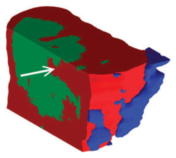
The reference viewpoint can be set to any arbitrary position and cut-aways of any planar surface allow inspection of the interior of the tumor. By looking at depth profiles along dimensions other than the z-axis, one can see how various ions are distributed in micro-encapsulated pockets (marked by white arrow) which might remain undetected when looking only at single-sections.

For a better understanding of the biology behind the identified components, we coupled ion abundance analysis with histological tissue staining to identify the detected sub-structures. One of the most prominent ions in regions 1 and 2 is detected at m/z 104.1, which is likely choline, a known tumor marker.^21–23 As the abundance of m/z 104.1 is significantly lower in region 3, this suggests that regions 1 and 2 together may represent the actual tumor mass (Fig. 4A, red), while region 3 might be formed by a different type of tissue (Fig. 4A, blue). Mouse mammary glands are known for their high content of fat.²⁴ To test for the presence of adipocytes in the analyzed tissue, we stained sections adjacent to the mass spectrometry sections with Oil Red O, a dye that selectively stains fat and lipids. Surprisingly, only a very small part of the tissue showed a positive Oil Red O stain (Fig. 4B). But most interestingly, the stained portion fits exactly to the tissue area described by region 3 (Fig. 4A, blue). This data suggests that region 3 represents fat tissue on the edge of the tumor. For a more detailed analysis of the tumor tissue described by regions 1 and 2, the histology of the imaged tissue was further analyzed by H&E stains of sections adjacent to the imaged sections. For example, Fig. 5 shows the localization of region 2 (Fig. 5A) and an H&E stain (Fig. 5B) for section 24. In general, the hematoxylin staining is dominant throughout the whole tissue, revealing relatively small and densely packed cells. This also shows that with the exception of the detected fat tissue most of the tissue is formed by tumor cells. However, the H&E stain also clearly shows that the cell density is higher on the left side of the tissue, peaking in the area of the tissue that is equivalent to region 2 (Fig. 5A). Magnifications of small areas from the left side of the tissue within region 2 (Fig. 5C) and from the right side within region 1 (Fig. 5D) show the differences in cell density in a more detailed way. These data suggest that regions 1 and 2 represent the same general tissue type (i.e. the tumor), but due to putative differences in the microenvironment, form different populations within the tissue; this is evidenced by their unique ion profiles.

Fig. 4. Identification of tumor and fat cells.

(A) An ion at m/z 104.1, which is likely to be choline, can be used to distinguish the tumor regions. Red in the model represents high abundance of the ion at m/z 104.1 (equivalent to regions 1 and 2 in Fig. 3D), blue represents an area with high levels of an ion at m/z 198.1 (equivalent to region 3 in Fig. 3D), which exists only at low abundance in the red region. (B) Oil Red O stained tissue section 23 reveals the localization of adipocytes at the edge of the tumor. The staining matches the localization of region 3. Scale bar represents 2 mm.

Fig. 5. Histological analysis of the tumor tissue.

The detected regions match morphological characteristics identified by H&E staining. (A) Localization of region 2 in tissue section 24. (B) H&E stain of tissue section 24 revealing different cell densities within the tissue. Dashed box shows tissue section enlarged in panel C, dotted box shows tissue section enlarged in panel D. Scale bar represents 2 mm. (C) Enlarged image of cells from region 2 shows high cell density. (D) Enlarged image of cells from region 1 shows low cell density.

Cutting away several virtual planes from the 3D reconstruction to show the three identified regions allowed a more detailed view of spatial sub-structures inside the tissue (Fig. 6). The possibility to access every plane inside the 3D image allows for a precise analysis of ion abundances in the context of any surrounding tissue parts. This presents an important advantage in comparison to 2D tissue analysis, which is limited in explaining the effects of tissues above and below the imaged section. For example, if the tissue localization marked by the arrow in Fig. 6 would be analyzed as an isolated 2D image any observed effects would be attributed to region 1 (Fig. 6, red). However, the 3D image shows that the marked position lies directly adjacent to region 2 (Fig. 6, green). Any effects at the marked position in region 1 could be directly influenced by region 2. Therefore, to understand the molecular effects in tissue it is important to consider the full 3D space for physiological relevance.

Discussion

There are several challenges associated with multivariate statistical analysis on 3D mass spectrometry imaging datasets. For example, isolated multivariate analyses of individual sections cannot be accurately assembled into a 3D multivariate reconstruction and must be performed simultaneously on the complete 3D dataset. Additionally, the computational challenges associated with processing dozens of sections (each comprised of many gigabytes of data) have prevented the use of this approach to 3D mass spectral imaging. We overcame these challenges by generating a coherent 4D matrix (x, y, z, m/z) of intensity values. This coherent matrix describes the intensity for each ion in 3 spatial dimensions, and was generated by (1) sparse matrices for initially loading and storing all x, y, m/z information for each section; (2) integrating all data into a total mass spectrum; (3) identification of the top 200 ions present in the dataset; (4) construction of a single 4D dataset of intensities (x, y, z, m/z); (5) perform NMF on this matrix to identify components within the 3 spatial dimensions; and (6) export visualizations of intensity projections along each axis and 3D volume reconstructions defined by each component (Fig. 3).

The most challenging and important aspect of the above workflow was the construction of the 4D dataset because all intensity values must be registered on defined x, y, z, m/z axes. Without this alignment step one would be comparing the same ions, albeit slightly shifted in m/z, as if they were unique ions. Similarly, one could mistakenly compare ions in sequential sections that are not spatially registered. To illustrate this point, it is known that in some cases ions shift in m/z as a result of minor changes in tissue properties, making it difficult to maintain high mass accuracy and detection of the same ion as multiple m/z across tissue sections. Multivariate analysis could mistakenly define a component based on the similar spatial distribution of these seemingly unique ‘ions’, actually referring to only one single ion. Since the purpose of multivariate statistics is to discover regions and clusters of ions for subsequent analysis, we have used the strategy of binning ion intensities to minimize the effects of shifting m/z, though it does require subsequent analysis to confirm accurate mass.

Many groups have described the use of marker points for image registration.²⁵ This is particularly useful for alignment of histological images with mass spectral images, particularly of brain regions which have clear anatomical features to aid alignment.¹⁸ However, this method is not as well suited for alignment of tumor sections which have less clear morphological features. Therefore, we have employed an automated image registration approach that is based on the correlation of ion intensities between sequential sections. Optimization proceeds by exploring the x and y shifts and rotation of the x-y plane about the z-axis. This process, like most optimizations, is prone to finding false minima. For this reason, we have employed the Pattern Search algorithm that overcomes this limitation and find the global optimum.²⁶ Using this approach, a 143% improvement in the correlation was achieved after re-locating the image.

Multivariate statistical analysis was performed on the resulting coherent 4D dataset. While principle component analysis (PCA) has been the most widely used multivariate analysis technique, we have found it preferable to use non-negative matrix factorization (NMF) because all of the spectral loadings are positive and easier to interpret. This technique has historically been used for a variety of applications including interpreting complex spectra.²⁷ The appearance of the NMF results has the same format as a mass spectrum and can therefore be easily interpreted.

The resulting statistically analyzed and surface rendered 3D image provides a detailed view of variations in the tumor, which has several advantages over conventional 2D image analysis. Fig. 6 shows that region 2 (green) was not detected in the bottom tissue sections. If tissue analysis would have been based solely on one or only very few 2D sections from that part of the tissue, a whole molecular sub-population would not have been detected. Furthermore, local sub-structures in individual sections might be misinterpreted in a 2D context. For example, small sub-structures in a 2D section, that seem to be of minor influence on the whole sections, might be part of a much bigger structure across the whole 3D tissue (e.g. vasculature). Therefore the 3D reconstruction is a more realistic view of the microenvironment by linking physiological structures above and below individual slices that may influence the observed phenotype of any individual section. Therefore, 2D tissue analysis is somewhat dependent on the random selection of an appropriate representative tissue section. To some extent this is also true for the 3D sampling; if a tumor is excised imprecisely, sub-populations can also be missed out. However, we think that by the analysis of a 3D model such imprecisions can be detected in a much clearer way as in an isolated 2D section. For example when one identified component sits at the very edge across several sections of the imaged tissue and was obviously split by the excision. This might have happened for the identified region 3, representing the fat tissue. Using our approach, complete tumor excision would be seen as one component representing the tumor mass being completely surrounded by normal stromal cells. To this end, the analysis of non-tumorous control tissue would be beneficial to define the molecular background for the type of analyzed tissue. Unfortunately, control tissue was not available for this study.

The resolution of the acquired 3D image is 75 μm, both in x- and y-direction, and 28 μm in z-direction. With cell sizes of 10 μm and more, this means that the resolution is not high enough for the analysis of single cells or of a detailed cellular microenvironment. However, this resolution is below the focus of current commercial instrumentation. Therefore, this study was mainly focused on developing the automated statistical analysis of 3D imaging data required to study the tissue microenvironment. For that purpose the resolution was high enough; different cell types and cellular environments could be detected. In comparison to conventional 3D analysis techniques, the big advantage of the presented method is direct label-free detection of analytes. In 3D microscopy for example, a very limited number of molecules can be detected in parallel through tagging with exogenous labels. In a mass spectrometric approach up to several thousand molecules can be analyzed simultaneously. Therefore, the output of data from a single experiment has the potential to greatly exceed any conventional 3D imaging technique.

Conclusions

In summary, we present the 3D reconstruction of a mouse mammary tumor and, to our knowledge, the first application of multivariate statistical analysis to a 3D mass spectral image. The statistical analysis revealed several components within the tissue. Parallel analysis of adjacent sections with biological tissue stains confirmed the identified components. The combination of 3D reconstruction and multivariate analysis should be of great use in studying the various microenvironments and the heterogeneity of tumorous tissue. In 2D image analysis several sub-populations might be identifiable within a single tissue section, but this only presents a 2D snapshot and the importance of certain clusters might be over- or underestimated. The 3D model has the advantage of evaluating the tissue in its physiological context which allows a more detailed understanding of any observed phenotypes.

Materials and methods

Fabrication of the mass spectrometry surface

The preparation of nanostructure-initiator mass spectrometry (NIMS) surfaces has been described in detail elsewhere.²⁸ In brief, a 4″ silicon wafer (single-sided polished P/Boron, orientation 〈1-0-0〉, resistivity 0.01–0.02 Ωcm, thickness 525 ± 25 μm) obtained from Silicon Quest International (Santa Clara, CA) was cut into a 70 × 70 mm square, washed in Piranha solution (sulfuric acid/hydrogen peroxide), and etched with 25% hydrofluoric acid in ethanol in a custom made Teflon etching chamber under constant current of 2.4 A for 15 min. After etching, chips were coated with 400 μl of initiator liquid (bis(heptadecafluoro-1,1,2,2-tetrahydrodecyl)tetramethyl-disiloxane) purchased from Gelest (Morrisville, PA).

Tumor collection and sectioning

The mouse mammary tumor was dissected from a 5 month old female C3(1)-SV40T/t-antigen transgenic mouse in the FVB/N background²⁹ and immediately frozen on dry ice. The tissue was subsequently stored at −80 °C until further use. Sectioning of the tissue was carried out on a CM3050S Cryostat from Leica Microsystems (Bannockburn, IL). Sections were cut directly from frozen tissue at a thickness of 7 μm. For imaging mass spectrometry a total of 30 sections were cut every 28 μm in the z-direction and thaw-mounted onto the mass spectrometry surface, so that a tissue thickness of ~1 mm was covered. Additionally, in each case two more 7 μm sections directly following the sections used for mass spectrometry were thaw-mounted onto glass slides and used for H&E and Oil Red O stainings.

Tissue staining

One set of sequential sections was subject to hematoxylin and eosin (H&E) staining. To this end, sections were fixed in 10% formalin (Azer Scientific; Morgantown, PA), followed by staining with Mayer’s hematoxylin solution (Dako; Carpinteria, CA), transfer into 80% ethanol, and staining with eosin solution (VWR; West Chester, PA). After subsequent washes in 80% ethanol, 95% ethanol, 100% ethanol, and xylene, slides were mounted using Permount mounting medium (Fisher Scientific; Pittsburgh, PA). Another set of sections was stained using Oil Red O. Sections were first fixed in 10% formalin (Sigma-Aldrich; St. Louis, MO), transferred into 60% isopropanol, and stained with a 3 mg ml⁻¹ solution of Oil Red O (Sigma-Aldrich; St. Louis, MO) in 60% isopropanol. After rinsing with 60% isopropanol, slides were mounted with VectaShield mounting medium (Vector Labs; Burlingame, CA). For both stainings microscopy was performed on a MZ16 stereomicroscope and images were recorded on a DFC420 camera from Leica Microsystems (Bannockburn, IL).

Imaging mass spectrometry

Nanostructure-initiator mass spectrometry (NIMS) was performed on a 5800 TOF/TOF mass analyzer system (AB Sciex; Foster City, CA) in positive reflector mode. The third harmonic of a Nd:YAG laser (355 nm) was used at a repetition rate of 200 Hz with 25 shots per spot. A full mass spectrum ranging from 50 to 2000 m/z was recorded for every position at an x-y step-size of 75 μm, so that a final resolution of 75 (x) × 75 (y) × 28 (z) μm was obtained. All sections were imaged with identical settings. Imaging data was stored in the Analyze 7.5 data format (Mayo Foundation; Rochester, MN).

3D image reconstruction and statistical analysis

The following steps were used to integrate multiple 2D image files into a 3D reconstruction, subsequently followed by statistical analysis. All steps were performed using custom made scripts in the MATLAB (The MathWorks; Natick, MA) programming language.

Import of imaging data

A custom script was used to parse the Analyze 7.5 image files. The script read the spectra at each spatial coordinate of each 2D section and stored the intensity information in a 2D sparse array. The first dimension represents all the pixels, and the second dimension represents all the m/z values. The total size of this dataset across all 30 sections was 115 gigabytes.

Total 3D spectrum and peak finding

The major ions in the data stack were determined with the help of an integrated total 3D spectrum, whereas a defined m/z axis from 50 to 2000 in steps of 0.01 was chosen as the basis for registering all of the acquired spectra. After smoothing the total spectrum with a Gaussian point-spread function with a 0.2 Da standard deviation, the top 200 peaks in this spectrum were selected to represent the major ions in the data stack. All m/z values in each pixel were binned ±0.3 Da to compensate for any shifts in m/z that occurred over the imaging run.

Image processing

For each of the 200 ions, a 3D data stack was created. This stack was operated on by maximum intensity projections and total intensity projections in the x-y plane, the x-z plane, and the y-z plane, techniques typically used in 3D confocal fluorescence microscopy. All single section data and projections are available in the ESI (supplementary information 1).^‡

Section alignment and 3D image reconstruction

After examining the images for each of the 200 individual ions, representative ions can be seen that are most associated with the region of the image bounded by the tissue and the region of the image thought to be background. As acquired, data is only crudely spatially aligned in the sequential sections. An optimization approach was used to align each subsequent section with all preceding sections. The Pattern Search algorithm was used to find the maximum correlation between intensities in pixels. The Pattern Search algorithm is robust to avoiding local minima and is well suited for this type of problem.²⁶ Three variables were considered for section alignment: translation in x and y plus rotation of the x-y plane. The x and y translation was bounded to ±40 pixels and the rotation was bounded by ±20 degrees. All slices were padded with zeros to minimize edge effects. The zero-padding values were removed after optimum alignment of the stack was achieved. Aligned slices and projections for each of the major ions can be seen in the ESI (supplementary information 1).^‡ 3D images were created by defining an equal intensity surface and rendering it in the presence of a light source.

Multivariate statistical analysis

Non-negative matrix factorization (NMF) was used for the multivariate analysis. First, using the multiplicative update algorithm, twenty replicates were performed from random starting values. The best of these parameters was then used as the initial guess where the alternating least squares algorithm was used. The nonnegative factors, W and H, were used to represent regions of the data in a reduced dimension. W is a 397980 (x·y·z) by 30 matrix. H is a 200 by 30 matrix, where 30 is the number of dimensions specified in the factorized model and 200 is the number of ions chosen for analysis. W can be easily reshaped into a 134 (x) by 99 (y) by 30 (z) by 30 (factors) matrix for 3D visualization and analysis. H is the loadings matrix that shows the contribution of each of the 200 ions towards each of the 30 components.

Insight, innovation, integration.

The broad understanding of a tumor’s biology is only possible in the context of its microenvironment. Therefore, only techniques that can study the 3D structure of a tumor are able to map all the salient molecular processes. We apply automatic mass spectral image analysis for the generation and characterization of a 3D tumor reconstruction. Multivariate statistical analysis was used to identify different regions of the tumor. The presented technique is an approach to better understand the microenvironmental heterogeneity of tumorous tissue.

References

- 1.Mbeunkui F, Johann DJ., Jr Cancer Chemother Pharmacol. 2009;63:571–582. doi: 10.1007/s00280-008-0881-9. [DOI] [PMC free article] [PubMed] [Google Scholar]
- 2.Weaver VM, Fischer AH, Peterson OW, Bissell MJ. Biochem Cell Biol. 1996;74:833–851. doi: 10.1139/o96-089. [DOI] [PMC free article] [PubMed] [Google Scholar]
- 3.Ghajar CM, Bissell MJ. Histochem Cell Biol. 2008;130:1105–1118. doi: 10.1007/s00418-008-0537-1. [DOI] [PMC free article] [PubMed] [Google Scholar]
- 4.Weigelt B, Lo AT, Park CC, Gray JW, Bissell MJ. Breast Cancer Res Treat. 2010;122:35–43. doi: 10.1007/s10549-009-0502-2. [DOI] [PMC free article] [PubMed] [Google Scholar]
- 5.Heppner GH. Cancer Res. 1984;44:2259–2265. [PubMed] [Google Scholar]
- 6.Marusyk A, Polyak K. Biochim Biophys Acta. 2010;1805:105–117. doi: 10.1016/j.bbcan.2009.11.002. [DOI] [PMC free article] [PubMed] [Google Scholar]
- 7.Neve RM, Chin K, Fridlyand J, Yeh J, Baehner FL, Fevr T, Clark L, Bayani N, Coppe JP, Tong F, Speed T, Spellman PT, DeVries S, Lapuk A, Wang NJ, Kuo WL, Stilwell JL, Pinkel D, Albertson DG, Waldman FM, McCormick F, Dickson RB, Johnson MD, Lippman M, Ethier S, Gazdar A, Gray JW. Cancer Cell. 2006;10:515–527. doi: 10.1016/j.ccr.2006.10.008. [DOI] [PMC free article] [PubMed] [Google Scholar]
- 8.Chin K, DeVries S, Fridlyand J, Spellman PT, Roydasgupta R, Kuo WL, Lapuk A, Neve RM, Qian Z, Ryder T, Chen F, Feiler H, Tokuyasu T, Kingsley C, Dairkee S, Meng Z, Chew K, Pinkel D, Jain A, Ljung BM, Esserman L, Albertson DG, Waldman FM, Gray JW. Cancer Cell. 2006;10:529–541. doi: 10.1016/j.ccr.2006.10.009. [DOI] [PubMed] [Google Scholar]
- 9.Varley KE, Mutch DG, Edmonston TB, Goodfellow PJ, Mitra RD. Nucleic Acids Res. 2009;37:4603–4612. doi: 10.1093/nar/gkp457. [DOI] [PMC free article] [PubMed] [Google Scholar]
- 10.Lunt SJ, Chaudary N, Hill RP. Clin Exp Metastasis. 2009;26:19–34. doi: 10.1007/s10585-008-9182-2. [DOI] [PubMed] [Google Scholar]
- 11.Warburg O, Wind F, Negelein E. J Gen Physiol. 1927;8:519–530. doi: 10.1085/jgp.8.6.519. [DOI] [PMC free article] [PubMed] [Google Scholar]
- 12.Warburg O. Science. 1956;123:309–314. doi: 10.1126/science.123.3191.309. [DOI] [PubMed] [Google Scholar]
- 13.Vander Heiden MG, Cantley LC, Thompson CB. Science. 2009;324:1029–1033. doi: 10.1126/science.1160809. [DOI] [PMC free article] [PubMed] [Google Scholar]
- 14.Svatos A. Trends Biotechnol. 2010;28:425–434. doi: 10.1016/j.tibtech.2010.05.005. [DOI] [PubMed] [Google Scholar]
- 15.Chughtai K, Heeren RM. Chem Rev. 2010;110:3237–3277. doi: 10.1021/cr100012c. [DOI] [PMC free article] [PubMed] [Google Scholar]
- 16.Fletcher JS, Lockyer NP, Vaidyanathan S, Vickerman JC. Anal Chem. 2007;79:2199–2206. doi: 10.1021/ac061370u. [DOI] [PubMed] [Google Scholar]
- 17.Eberlin LS, Ifa DR, Wu C, Cooks RG. Angew Chem, Int Ed. 2010;49:873–876. doi: 10.1002/anie.200906283. [DOI] [PMC free article] [PubMed] [Google Scholar]
- 18.Andersson M, Groseclose MR, Deutch AY, Caprioli RM. Nat Methods. 2008;5:101–108. doi: 10.1038/nmeth1145. [DOI] [PubMed] [Google Scholar]
- 19.Trim PJ, Atkinson SJ, Princivalle AP, Marshall PS, West A, Clench MR. Rapid Commun Mass Spectrom. 2008;22:1503–1509. doi: 10.1002/rcm.3498. [DOI] [PubMed] [Google Scholar]
- 20.McDonnell LA, van Remoortere A, van Zeijl RJ, Dalebout H, Bladergroen MR, Deelder AM. J Proteomics. 2010;73:1279–1282. doi: 10.1016/j.jprot.2009.10.011. [DOI] [PubMed] [Google Scholar]
- 21.Sijens PE, Oudkerk M. Eur Radiol. 2002;12:2056–2061. doi: 10.1007/s00330-001-1300-3. [DOI] [PubMed] [Google Scholar]
- 22.Herminghaus S, Pilatus U, Moller-Hartmann W, Raab P, Lanfermann H, Schlote W, Zanella FE. NMR Biomed. 2002;15:385–392. doi: 10.1002/nbm.793. [DOI] [PubMed] [Google Scholar]
- 23.Bartella L, Morris EA, Dershaw DD, Liberman L, Thakur SB, Moskowitz C, Guido J, Huang W. Radiology. 2006;239:686–692. doi: 10.1148/radiol.2393051046. [DOI] [PubMed] [Google Scholar]
- 24.Pitelka DR, Hamamoto ST, Duafala JG, Nemanic MK. J Cell Biol. 1973;56:797–818. doi: 10.1083/jcb.56.3.797. [DOI] [PMC free article] [PubMed] [Google Scholar]
- 25.Walch A, Rauser S, Deininger SO, Hofler H. Histochem Cell Biol. 2008;130:421–434. doi: 10.1007/s00418-008-0469-9. [DOI] [PMC free article] [PubMed] [Google Scholar]
- 26.Hooke R, Jeeves TC. J ACM. 1961;8:212–229. [Google Scholar]
- 27.Lawton WH, Sylvestre EA. Technometrics. 1971;13:617–633. [Google Scholar]
- 28.Northen TR, Yanes O, Northen MT, Marrinucci D, Uritboonthai W, Apon J, Golledge SL, Nordstrom A, Siuzdak G. Nature. 2007;449:1033–1036. doi: 10.1038/nature06195. [DOI] [PubMed] [Google Scholar]
- 29.Maroulakou IG, Anver M, Garrett L, Green JE. Proc Natl Acad Sci U S A. 1994;91:11236–11240. doi: 10.1073/pnas.91.23.11236. [DOI] [PMC free article] [PubMed] [Google Scholar]
Associated Data
This section collects any data citations, data availability statements, or supplementary materials included in this article.