

Abstract
Motivation: RNA-Seq uses the high-throughput sequencing technology to identify and quantify transcriptome at an unprecedented high resolution and low cost. However, RNA-Seq reads are usually not uniformly distributed and biases in RNA-Seq data post great challenges in many applications including transcriptome assembly and the expression level estimation of genes or isoforms. Much effort has been made in the literature to calibrate the expression level estimation from biased RNA-Seq data, but the effect of biases on transcriptome assembly remains largely unexplored.
Results: Here, we propose a statistical framework for both transcriptome assembly and isoform expression level estimation from biased RNA-Seq data. Using a quasi-multinomial distribution model, our method is able to capture various types of RNA-Seq biases, including positional, sequencing and mappability biases. Our experimental results on simulated and real RNA-Seq datasets exhibit interesting effects of RNA-Seq biases on both transcriptome assembly and isoform expression level estimation. The advantage of our method is clearly shown in the experimental analysis by its high sensitivity and precision in transcriptome assembly and the high concordance of its estimated expression levels with quantitative reverse transcription–polymerase chain reaction data.
Availability: CEM is freely available at http://www.cs.ucr.edu/~liw/cem.html.
Contact: liw@cs.ucr.edu
Supplementary information: Supplementary data are available at Bioinformatics online.
1 INTRODUCTION
RNA-Seq, or deep sequencing of RNAs, takes the advantage of recent high-throughput sequencing methods to detect and quantify transcriptomes (Mortazavi et al., 2008). The RNA-Seq technology is becoming a standard and fundamental protocol in transcriptomic research and has successfully been applied to study different organisms, diseases and cancers. Various bioinformatics algorithms and tools have been developed for RNA-Seq data analysis, including read mapping and junction discovery (Au et al., 2010; Trapnell et al., 2009), the expression level estimation of genes/isoforms and differential expression analysis (Langmead et al., 2010; Mortazavi et al., 2008), transcriptome assembly from mapped reads (e.g. Feng et al., 2010; Guttman et al., 2010; Li et al., 2011a, b; Trapnell et al., 2010) or de novo assembly (e.g. Birol et al., 2009; Grabherr et al., 2011; Peng et al., 2011), etc. Despite the success of these RNA-Seq applications, many challenges remain in the analysis of RNA-Seq data, one of which comes from the understanding and handling of biases in RNA-Seq data.
The term ‘bias’ refers to the non-random, non-uniform distribution of the sequenced fragments (or ‘reads’) across the involved isoforms [or messenger RNA (mRNA) transcripts] in an RNA-Seq experiment. Both positional (Dohm et al., 2008; Mortazavi et al., 2008) and sequencing biases (Hansen et al., 2010; Li et al., 2010b) are routinely observed in RNA-Seq experiments. Positional bias is the non-uniform distribution of reads over different positions of a transcript, while sequencing bias refers to the distribution of reads related to the sequence content and priming method (Li et al., 2010b). Since many next-generation sequencing applications (including RNA-Seq) require the mapping of reads to the reference genome, the mappability bias is also an important source of biases in RNA-Seq and ChIP-Seq (Rozowsky et al., 2009; Schwartz et al., 2011). The mappability bias arises when read counts are biased due to read mapping. For example, some reads may not be mapped due to sequencing errors and some applications discard reads mapped to the repeat regions of the reference genome; the numbers of reads are thus under-counted for these regions. Also, incorrect read mapping leads to incorrect read counts for regions where the involved reads are mapped to.
Biases in RNA-Seq data may cause inaccurate expression level estimation of genes (or isoforms), where most bias correction methods try to overcome. For example, positional biases are handled by learning non-uniform read distributions from given RNA-Seq reads or modeling the RNA degradation (Wan et al., 2012; Wu et al., 2011). In Srivastava and Chen (2010), a generalized Poisson (GP) model is used to calculate the expression levels of genes affected mainly by sequencing biases. Other approaches include checking the repeat regions of the reference genome to handle mappability biases (Lee et al., 2010; Richard et al., 2010), modeling the dependency between neighboring positions to correct sequencing biases (Li et al., 2010b) or a combination of several strategies (Roberts et al., 2011). However, some methods can handle only one specific type of biases (e.g. Richard et al., 2010; Wu et al., 2011) or correct biases only at the gene level (Srivastava and Chen, 2010). Other more general methods use sophisticated probabilistic generative models that require the learning of a large number of parameters and thus have to make some simplifying assumptions to make the computation tractable (Li et al., 2010b; Roberts et al., 2011).
Besides expression level estimation, the RNA-Seq biases also have significant effects on transcriptome assembly. For example, RNA-Seq biases may generate ‘gap regions’ on the reference genome where no mapped reads are observed. Because of these gaps, two broken transcripts may be assembled instead of one complete transcript. Also, incorrectly mapped reads may lead to incorrect transcript assemblies. As far as we know, most work in the literature concerning RNA-Seq biases deal with correcting gene (or isoform) expression level estimation, and the effects of biases on the transcriptome assembly remain largely unexplored.
In this article, we propose a statistical framework based on the quasi-multinomial distribution model (Consul and Jain, 1973; Consul and Mittal, 1977) to capture the above-mentioned RNA-Seq biases, including positional, sequencing and mappability biases. The framework allows us to develop an expectation–maximization (EM) algorithm (Dempster et al., 1977; Nicolae et al., 2010) for both transcriptome assembly and isoform abundance level estimation from biased RNA-Seq data. Compared with other algorithms in the literature that use sophisticated probabilistic generative models to handle biases, our EM algorithm uses a single parameter to capture the property of RNA-Seq biases of different types. Utilizing the isoform enumeration algorithm of IsoLasso (Li et al., 2011b), the EM algorithm assembles isoforms and estimates their abundance levels at the same time. Moreover, both principles of prediction accuracy and interpretation (or ‘sparsity’) considered in Li et al. (2011b) are achieved in the assembly.
The statistical framework and the EM algorithm are introduced in Sections 2 and 3, we demonstrate the superior performance of our EM algorithm compared with other algorithms in the literature through simulated and real RNA-Seq experiments and analyze the effects of RNA-Seq biases on both transcriptome assembly and isoform abundance level estimation. Due to the page limit, we defer some figures and technical derivations to the Supplementary Materials.
2 METHODS
2.1 The quasi-multinomial model for isoform abundance level estimation
Consider a gene G consisting of M exons with length  (or more generally, the so-called ‘expressed segments’ as defined in Feng et al. (2010), each of which is a contiguous region of the reference genome not separated by any exon–intron boundary). If G induces N isoforms (denoted as
  ), then these isoforms can be represented as an
  binary matrix
  , where
  if isoform ti includes exon (or expressed segment) j, and 0 otherwise. Let
  be the random variable of the read counts falling into exon j. Under the assumption that a read r is sampled uniformly from an isoform (the ‘Poisson assumption’),
  follows a Poisson distribution with parameter
  proportional to the length of exon j and the total abundance level of all isoforms containing exon j (Jiang and Wong, 2009). The abundance level is usually measured by RPKM (Mortazavi et al., 2008) or FPKM (Trapnell et al., 2010) and can be estimated by maximizing the joint probability of observing
  reads in M exons, as proposed in Jiang and Wong (2009).
In the following, we develop a quasi-multinomial model (Consul and Mittal, 1977) to capture biases in RNA-Seq data. Consider a single-end (or paired-end) read  of length L that is mapped to exon j of length
  from gene G. Denote
  as the prior probability that read
  comes from ti with the constraint
  . We may think of the process of sampling
  as follows: one of the isoforms ti is first randomly selected with probability
  and then a read
  belonging to exon j is sampled from ti with probability
  . To model positional (and other) biases, the probability
  can be defined as a distribution
  depending on the location
  of
of  in ti. Note that if f is the uniform distribution, then
| (1) |
where  is the length of ti.
  can also be an exponential function to model the RNA degradation process which plays an important role in the formation of the positional bias (Wan et al., 2012).
Several strategies can be used to construct a non-uniform distribution f. For example, a non-uniform positional distribution can be determined empirically and incorporated into f (Wu et al., 2011). The ‘effective length’ of isoforms excluding repeat regions of the reference genome can be used in Equation (1) to handle mappability biases (Richard et al., 2010).
The probability of observing read  is thus
| (2) |
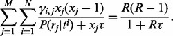
and the joint probability of observing R reads mapped to gene G follows a quasi-multinomial distribution:
 |
(3) |
where  is the bias parameter. The value of
  indicates how read counts differ from a multinomial distribution: if
  then too many reads are observed (called ‘over-dispersion’) and if
  (called ‘under-dispersion’), fewer reads are observed.
Note that the GP distribution  (Consul and Jain, 1973) is used in Srivastava and Chen (2010) for modeling RNA-Seq biases, where
  is the parameter to account for the biases. The GP model can also be used to estimate isoform expression levels. In fact, Equation (3) can be approximated by a product of M GP distributions (Consul and Mittal, 1977), and finding an optimal
  would be equivalent to finding an optimal
  in the GP model (see Supplementary Materials). However, the GP model uses only the information of read counts and it does not consider the fact that a read may come from different isoforms with different probabilities due to the sampling biases.
2.2 Transcriptome assembly
Transcriptome assembly (for a fixed gene) from mapped RNA-Seq reads usually generates a set of candidate isoforms (i.e. the isoform matrix  ), and then selects one or more of these candidates according to several criteria such as prediction accuracy, interpretation and completeness (Li et al., 2011b).
We use the candidate isoform enumeration algorithm introduced in IsoLasso (Li et al., 2011b), which is proven to generate the same set of candidate isoforms considered by Cufflinks (Trapnell et al., 2010). The algorithm first enumerates all possible paths in the connectivity graph (Guttman et al., 2010) constructed from the mapped reads. Then two additional steps are applied to remove infeasible paths and non-maximal paths.
IsoLasso uses the LASSO algorithm (Tibshirani, 1996) to select candidate isoforms and estimate their abundance levels. However, the LASSO algorithm is solved by constrained quadratic programming which could be very slow if many constraints are imposed. Moreover, it is unable to handle biases in RNA-Seq data. We will develop an EM algorithm (called component elimination EM) in the next section based on the above quasi-multinomial model to select candidate isoforms and estimate their abundance levels from biased RNA-Seq data. Note that EM algorithms are routinely used in RNA-Seq data analysis (e.g. Nicolae et al., 2010; Trapnell et al., 2010), and several EM algorithms have been proposed in the literature to use information beyond read counts to improve the accuracy of isoform abundance level estimation. For example, multi-reads (i.e. reads mapped to several locations of the reference genome) are utilized to estimate the abundance levels of isoforms (Li et al., 2010a) or homologous genes (Paşaniuc et al., 2010). Also, the distribution of the fragment length in paired-end RNA-Seq data can be incorporated into the EM algorithms to address the effect of fragment selection in RNA-Seq library preparation (Roberts et al., 2011; Salzman et al., 2011; Trapnell et al., 2010). Such information can be readily incorporated to our quasi-multinomial model and the EM algorithm (see Supplementary Materials).
2.3 Component elimination EM
It is commonly believed that a gene usually has only a few highly expressed isoforms (Li et al., 2011b). For this reason, ensuring a good interpretation (or ‘sparsity’) (Hastie et al., 2009) is critical in transcriptome assembly. Generally speaking, in the context of EM algorithm, a good interpretation is to keep the number of components (i.e. the number of models whose probabilities are to be determined in the algorithm) as small as possible (Figueiredo and Jain, 2002). However, if the number of isoforms (or components) is large, the standard EM algorithm may deliver results that lack sparsity, i.e. solutions with many components having small non-negative probabilities instead of solutions with only a few components having large probabilities while the others having zero probability (Figueiredo and Jain, 2002). To achieve sparsity, a negative Dirichlet prior distribution of  is added multiplicatively to the quasi-multinomial likelihood function in Equation (3) (Bicego et al., 2007; Figueiredo and Jain, 2002):
| (4) |
where  is the negative Dirichlet parameter specified by the user. The negative Dirichlet distribution assigns a higher probability if one or more of the values of
  are closer to 0 (see Supplementary Fig. S1). Hence, solutions with fewer non-zero values of
  are preferred.
The likelihood function is the product of Equations (3) and (4) (see Supplementary Materials). To obtain a maximum a posteriori estimation of  and
and  using EM, a latent binary variable
  is introduced to indicate whether a read
  comes from isoform ti,
  if
if  comes from isoform ti and 0 otherwise. In the E step of the EM algorithm, the expectation of
  , is evaluated using the current values of
  and
and  as follows:
| (5) |
And in the M step, by maximizing the joint likelihood function with respect to the constraint  is updated as (see Supplementary Materials for a detailed derivation):
| (6) |
where  .
.
The maximum likelihood estimation (MLE) value of  can be obtained using the following equation:
 |
(7) |
We use the Newton–Raphson method (Ypma, 1995) to calculate the value of  (see Supplementary Materials for details).
A component elimination EM algorithm (Bicego et al., 2007; Figueiredo and Jain, 2002) can be used to find solutions that favor a small number of highly expressed isoforms. Compared with the standard EM algorithm, it applies an additional component elimination step to exclude components with small probabilities. This method is able to determine the number of components automatically without having to invoke any model selection criteria such as the Bayesian Inference Criteria, Minimum Message Length principle, etc. During the EM iterations, a component elimination step eliminates isoform ti if  (or set
  ). Here, the negative Dirichlet parameter
  can be interpreted as the minimum number of reads required for each isoform to proceed to the next iteration. In this component elimination EM,
  is fixed to 0 once its value reaches <0 in Equation (6).
However, in some component elimination steps (especially at the beginning of the EM iterations), there could be too many (or all) components satisfying the elimination condition  . This is because the probability of each component is initialized randomly, which could be very small even for highly expressed isoforms if the number of components is large. Deleting all of them in one iteration may lead to a poor choice of components. As a result, we eliminate only one component with the minimum value of
  in each iteration.
The parameter  controls the number of isoforms to be output. The higher the value of
  is, the fewer isoforms are reported. Based on our empirical experience from simulation tests (Section 3), we set
  for a gene with R mapped reads in our experiments.
3 RESULTS
In this section, we test the algorithm on both simulated and real RNA-Seq data and compare its performance with two state-of-the-art algorithms for transcriptome assembly and isoform abundance level estimation that do not consider RNA-Seq biases [i.e. IsoLasso (Li et al., 2011b) and Cufflinks (Trapnell et al., 2010)], and a recent extension of Cufflinks that takes biases into account (Roberts et al., 2011). For convenience, we will refer to the last algorithm simply as ‘Cufflinks-bias’. To our best knowledge, Cufflinks-bias is the only algorithm in the literature that considers RNA-Seq biases and is capable of assembling transcriptome. Note that although SLIDE (Li et al., 2011a) was published after IsoLasso and Cufflinks, we do not compare with it here because it was only tested on Drosophila melanogaster transcriptome in Li et al. (2011a). During the comparison study, the parameters of all programs are tuned empirically to achieve their best performance.
3.1 Simulation
We simulate biased RNA-Seq reads as follows. Known isoforms from the mus musculus (mm9) annotation database are first downloaded from the UCSC genome browser (Fujita et al., 2011). Each isoform is then assigned a random abundance value that follows approximately a log-normal distribution (Alter et al., 2008; Bengtsson et al., 2005). Afterwards, different numbers of reads are generated from each isoform according to the assigned abundance. Sequencing errors and different positional biases are then simulated to generate the actual reads.
During the simulation, three different positional profiles are provided to determine the position of each read, and 80 million single-end reads are generated for each profile, including the uniform positional model (‘Uniform’ for short) and two Illumina positional bias models (Supplementary Fig. S2A). Both Illumina models reflect positional biases caused by different fragmentation methods, including complementary DNA (cDNA) fragmentation (or ‘cDNAf’) and RNA fragmentation (or ‘RNAf’) (Howard and Heber, 2010; Wang et al., 2009; Wu et al., 2011). We use the sequencing error profile in Dohm et al. (2008) to simulate sequencing errors (Supplementary Fig. S2B), where higher sequencing error is observed for positions at the end of a read.
The positional bias [i.e.  in Equation (2)] is learned from RNA-Seq data using a method similar to Wu et al. (2011). Basically, RNA-Seq reads are first mapped to the RefSeq transcript sequences using Bowtie (Langmead et al., 2009), where all possible mappings for each read are reported. A RefSeq sequence is selected to estimate its positional bias if the reads mapped to the sequence satisfy two conditions: (i) they cannot be mapped to other RefSeq sequences and (ii) the number of the reads is >1000. The average of the positional biases in these sequences (~2000) is then fed to the CEM algorithm. Supplementary Figure S3 demonstrates that the estimated positional biases from different datasets are close to the real positional biases.
3.1.1 Performance on transcriptome assembly
The performance of transcriptome assembly results is evaluated in terms of both sensitivity and precision, by comparing the predicted sets of isoforms with UCSC mm9 known isoforms (Hsu et al., 2006). A predicted isoform is matched to a known one if both isoforms include the same number of exons and their exon–intron boundaries are identical. If K of M predicted isoforms are matched to K out of N known isoforms, then the sensitivity and precision are defined as K/M [or  ] and K/N [or
  ], respectively.
To compare the effects of both positional and mappability biases on transcriptome assembly, we plot the sensitivity–precision curves in Figure 1 for four programs: CEM, IsoLasso (Li et al., 2011b), Cufflinks (Trapnell et al., 2010) and Cufflinks-bias (Roberts et al., 2011). Here, four different RNA-Seq reads are provided to the programs: reads with Uniform/cDNAf positional distributions and reads with/without mapping. For ‘reads without mapping’ (or ‘w/o mapping’ for short), the exact locations of the reads on the reference genome are provided; otherwise (‘reads with mapping’ or ‘mapping’ for short), simulated reads are mapped to the reference genome using Tophat (Trapnell et al., 2009) to obtain the locations of the reads. Compared with the ‘reads with mapping’ case, ‘reads without mapping’ serves as an ideal dataset which is not affected by mappability biases. Various values of sensitivity and precision in the curve are obtained by setting different abundance cutoffs used in the output of the programs. That is, for each cutoff, only predicted isoforms with estimated abundance levels higher than the cutoff value are output.
Fig. 1.

Sensitivity–precision curves of both CEM and Cufflinks-bias on four datasets (A) and a comparison of four different algorithms (B). 80 million 75 bp single-end RNA-Seq reads are generated, and Figure 1A shows the effect of both positional and mappability biases on CEM and Cufflinks-bias. Here, ‘w/o mapping’ means that correct read locations are provided and ‘mapping’ uses Tophat to map reads to the reference genome. Figure 1B compares four different programs for transcriptome assembly, including CEM, IsoLasso, Cufflinks and Cufflinks-bias. Here, the curves for CEM and Cufflinks-bias correspond to those in group 4 of Figure A
Figure 1A compares the curves of both CEM and Cufflinks-bias. When provided with the correct mapping information (i.e. w/o mapping), CEM and Cufflinks-bias both achieve high sensitivity ( ) and precision (
 ). A high abundance cutoff allows only a small number of highly expressed isoforms to be retained. These isoforms are more likely to be correct (than those lowly expressed ones), which leads to low sensitivity and high precision for both CEM and Cufflinks-bias (except in groups 3 and 4 due to reasons explained below). Compared with Cufflinks-bias, CEM achieves a better precision for the same level of sensitivity. CEM also performs best among all four algorithms, as seen in Figure 1B which shows the curves of all four algorithms using the cDNAf positional bias profile and ‘reads with mapping’ option.
Both non-uniform positional biases and inaccurate read mapping have negative impact on transcriptome assembly. Compared with non-uniform positional bias dataset, higher sensitivity and precision values are observed for data generated using the Uniform positional profile. Interestingly, positional biases mainly affect the inference of lowly and moderately expressed isoforms. This could be seen from the diminishing differences between the sensitivity–precision curves for data with the Uniform and cDNAf positional biases in Figure 1A (see groups 1 and 2 and the CEM curves in groups 3 and 4). The reason is that lowly expressed isoforms are less likely to have sufficient read coverage to be assembled completely, since their junctions are less likely to be fully covered by reads (Feng et al., 2010).
The values of sensitivity and precision decrease drastically when correct mapping is not guaranteed. Figure 1A shows a 10–15% decrease in sensitivity and a >20% decrease in precision in groups 3 and 4 compared with groups 1 and 2. Both repeat sequences of the genome and sequencing errors account for the decreased sensitivity and precision. This shows that mappability biases have a more profound effect on transcriptome assembly than positional biases. Different from positional biases, mappability biases affect both highly and lowly expressed isoforms.
Interestingly, Cufflinks-bias shows reduced performance in both sensitivity and precision in groups 3 and 4 on ‘reads with mapping’ for high abundance cutoffs. By inspecting the isoforms predicted by Cufflinks-bias carefully, we found that Cufflinks-bias is highly sensitive to mapping errors. For example, when the abundance cutoff is set as high as 500 FPKM, ~60% of the isoforms predicted by Cufflinks-bias come from regions with incorrectly mapped reads. Reads from the junctions of isoforms located in other regions could be mapped to these regions by TopHat because these junctions share identical sequences with those regions. As a result, the predicted isoforms are short compared with the read length, and Cufflinks-bias would greatly over-estimate their abundance levels, since it uses a fragment length model that assumes short fragments (short DNA sequences after fragmentation and before sequencing) are rare (Trapnell et al., 2010). A specific example is given in Supplementary Figure S4 and some statistics are given in Supplementary Figure S5. A similar observation of this behavior of Cufflinks is also reported recently in Li and Dewey (2011). CEM is less affected by this issue because it makes no assumption about the distribution of fragment lengths.
3.1.2 Longer read length improves both sensitivity and precision
To investigate the effect of read length on transcriptome assembly, we generate 80 million simulated reads of various read lengths (from 32 to 200 bp) using the uniform positional model (i.e. without positional biases) and compare both values of sensitivity and precision of two programs (CEM and Cufflinks, especially on read with mapping) in Figure 2. Here, no abundance cutoff is applied to the results of either program.
Fig. 2.
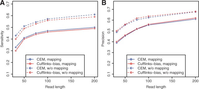
The effect of read length on both sensitivity (A) and precision (B)
Figure 2 shows that both sensitivity (A) and precision (B) increase as longer reads are used for assembly. However, such improvements tend to slow down as reads get longer. For example, when read length increases from 32 to 50 bp, the sensitivity of CEM (on reads with mapping) increases from 0.35 to 0.41. This increase is much more drastic than the improvement obtained when increasing read length from 100 to 200 bp, which is only around 0.03. Similar trends can be observed for Cufflinks (on reads with mapping) and for the value of precision.
Longer reads incur less ambiguity in mapping to the reference genome. For example, among all 32 bp reads mapped to the reference genome, 25% can be mapped to multiple locations. But for the 200 bp reads, only 12% are mapped to more than one location in the reference genome. However, in spite of the reduced ambiguity in mapping when longer reads are used, the differences in sensitivity and precision of both programs on reads with/without mapping are consistently observed in Figure 2 (which is always ~0.1). This shows that even for long reads, the mappability bias still affects the accuracy of transcriptome assembly.
3.1.3 Performance in abundance level estimation
We assemble transcripts from simulated RNA-Seq reads using the above algorithms, and then match their results to known mouse isoforms. For the matched isoforms, we compare the logarithms of the predicted and true abundance levels in Table 1 using coefficient of determination (i.e. the R2-value).
Table 1.
Comparison of the R2-values of the four algorithms in isoform abundance estimation on data with various positional biases
| Dataseta | CEM | IsoLasso | Cufflinks | Cufflinks-bias |
|---|---|---|---|---|
| Uniform | 0.90 | 0.87 | 0.86 | 0.89 |
| RNAf | 0.87 | 0.80 | 0.83 | 0.84 |
| cDNAf | 0.84 | 0.72 | 0.76 | 0.82 |
aAll R2 measurements have p-value < 2.2e-16 using Pearson's correlation test.
As shown in the table, all algorithms achieve high precision in abundance estimation on both Uniform and RNAf datasets ( ), but CEM outperforms the other three methods on all datasets. The cDNAf positional profile contains more biases compared with the RNAf profile, since it has a more extreme head and tail positional distribution as shown in Supplementary Figure S2A. Not surprisingly, lower R2-value is obtained for all methods on data with cDNAf positional biases. On the other hand, Cufflinks-bias demonstrates a clear advantage over Cufflinks on data with cDNAf positional biases.
3.2 Real data analysis
3.2.1 Correlation with microarray quality control data
We compare the abundance estimations for the microarray quality control (MAQC) (MAQC Consortium, 2006) Human Brain Reference (HBR) sample between Taqman quantitative reverse transcription–polymerase chain reaction (qRT–PCR) measurements and RNA-Seq analysis. The RNA-Seq reads and qRT–PCR measurements are downloaded from the NCBI SRA archive (accession number SRA012427) and Gene Expression Omnibus (accession number GSE5350), respectively. Since Taqman qRT–PCR only measures the expression levels of genes, we only compare gene abundance estimations between RNA-Seq and qRT–PCR. In RNA-Seq, the expression level of a gene is obtained by summing up the abundance levels of all isoforms induced by the gene.
Among 1097 Taqman qRT–PCR measurements of genes, 289 and 276 are correctly assembled by CEM and Cufflinks-bias, respectively, as shown in Figure 3A. The intersection of both programs covers 251 transcripts ( %), showing a high consistency between both methods. CEM recovers slightly more (13) transcripts than Cufflinks-bias. For the 38 and 25 transcripts uniquely assembled by CEM and Cufflinks-bias, Figure 3B plots the distribution of their qRT–PCR measurements. A few highly expressed transcripts are correctly assembled by CEM but not by Cufflinks-bias (for example, the isoforms of the AES gene shown in Supplementary Fig. S6).
Fig. 3.
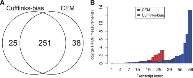
Comparison of the transcriptome assembly results between CEM and Cufflinks-bias. (A) The assembled transcripts by CEM and Cufflinks-bias match 289 and 276 of the 1097 Taqman qRT–PCR transcripts, respectively. (B) The distributions of the qRT–PCR measurements of the 38 and 25 transcripts uniquely assembled by CEM and Cufflinks
To compare the abundance estimations, we run the four algorithms in two different ways. In the first case (the ‘de novo’ approach), the algorithms are invoked to assemble transcripts and the results are matched against the known structures of RefSeq transcripts corresponding to Taqman gene measurements. (Note that here the term ‘de novo’ has a different meaning than it does in ‘de novo assembly’.) The abundance levels are compared with qRT–PCR measurements only for the matched genes. In the second case (the ‘refonly’ approach), the structures of all Taqman transcripts are provided, and the estimated abundance levels of all genes are compared with qRT–PCR measurements.
Figure 4 shows the R2-values between RNA-Seq and Taqman qRT–PCR measurements for both ‘de novo’ and ‘refonly’ approaches. We first compare the R2-values of the top 100 predicted highly expressed genes in Figure 4A (note that different numbers of genes between 50 and 200 give similar results). For these genes, the ‘de novo’ approach shows higher values of R2 than the ‘refonly’ approach. And among the four compared methods, CEM achieves the highest correlation.
Fig. 4.
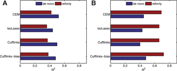
The R2-values between RNA-Seq and Taqman qRT–PCR measurements of the MAQC HBR sample for the top 100 predicted highly expressed genes (A) and for all genes (B)
However, when comparing RNA-Seq-based abundance estimations of all genes (instead of only highly expressed genes), Cufflinks-bias shows a clear improvement over Cufflinks as shown in Figure 4B and achieves the highest correlation among all four algorithms. This increased performance of Cufflinks-bias suggests that Cufflinks-bias corrects biases the best in the estimation of the abundance levels of moderately and lowly expressed genes, while CEM algorithm works the best for highly expressed genes. This is consistent with the observed advantage of CEM in the simulated data experiments.
The expression levels of genes also have an impact on the performance of the ‘de novo’ and ‘refonly’ approaches. For the 100 genes with the highest predicted expression levels, the R2-values from the ‘de novo’ approach are higher than those obtained by ‘refonly’ approach where known transcript structures are provided. However, for all genes, a large improvement in R2-values is observed for the ‘refonly’ approach over the ‘de novo’ approach as shown in Figure 4B. This suggests that knowing correct transcript structures is crucial for estimating the expression levels of lowly and moderately expressed genes, since it might be difficult for the algorithms to correctly assemble the isoforms of these genes from RNA-Seq reads.
We also analyze the regression line between RNA-Seq and Taqman qRT–PCR measurements in Table 2. The regression slope reflects the fold change between the expression levels of genes, where the ideal slope of 1.0 indicates that two methods are perfectly consistent in detecting fold changes between genes. Table 2 shows that although the R2-values are relatively low for the top 100 genes using the ‘refonly’ approach, CEM, IsoLasso and Cufflinks are able to detect fold changes quite accurately (slope  ). On the other hand, Cufflinks-bias is unable to match the performance on these highly expressed genes (slope = 0.75) for some reason (e.g. perhaps due to incorrect correction of their expression levels). Table 2 also shows that providing transcript structures helps the fold change detection (the slopes in the refonly columns are >0.75 while the slopes in the ‘de novo’ columns are only between 0.4 and 0.5).
Table 2.
The regression lines between RNA-Seq (y) and Taqman qRT–PCR measurements (x) in log scale
| Algorithm | Refonly top 100 | De novo top 100 | Refonly | De novo |
|---|---|---|---|---|
| CEM | 0.97 x + 5.8 | 0.42x + 3.8 | 0.71x + 5.8 | 0.54x + 3.4 |
| IsoLasso | 0.90x + 5.7 | 0.40x + 3.7 | 0.72x + 5.9 | 0.53x + 3.3 |
| Cufflinks | 0.92x + 3.1 | 0.43x + 3.0 | 0.72x + 3.2 | 0.53x + 3.3 |
| Cufflinks-bias | 0.76x + 2.0 | 0.43x + 3.5 | 0.73x + 3.0 | 0.55x + 3.8 |
Supplementary Figure S7 compares the running times of all four algorithms for processing 80 M paired-end reads on a Linux machine with 16 G memory and 2.6 GHz 8-core CPU. Since both Cufflinks and Cufflinks-bias provide the option of multithreading (‘-p’ option), we also include the results of both Cufflinks and Cufflinks-bias using four threads. We can see that for both Cufflinks and Cufflinks-bias, using multiple threads greatly reduces the processing time needed: only about one-fourth of the time is required for four threads compared with one thread. This is partly because transcriptome assembly can be trivially performed in parallel, allowing reads mapped to different genes to be processed simultaneously. If only a single thread is used, the speeds of all algorithms are approximately at the same level, with CEM slightly leading the edge.
3.2.2 Exon inclusion ratio analysis
The exon inclusion ratio (or ‘percent spliced in’ value,  ) measures the percentage of mRNA transcripts that include an exon to the total amount of transcripts that include or exclude that exon. The Ψ-value is frequently used to study the mechanism of alternative splicing (Pan et al., 2004; Wang et al., 2008; Xiao et al., 2009). In Xiao et al. (2009), both qRT–PCR and mRNA-Seq experiments are performed to measure the Ψ-values for human HEK 293T cells, including hnRNP H knockdown (or ‘KD’) cells and corresponding control (or ‘CTRL’) cells. RNA-Seq reads are first mapped to the human reference genome, and the Ψ-value is calculated as
 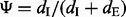 , where
  (inclusion density) is defined as the read density of the test exon and its two flanking junctions and
  (exclusion density) is the read density of the exclusion junction formed by the two flanking exons (see Supplementary Fig. S8). However, this method (called the ‘direct’ method) is sensitive to the value of
  , which may not be accurate if few reads are mapped to the exclusion junction. Alternatively, the Ψ-value can be calculated based on the abundance levels of two isoforms including and excluding the test exon:
 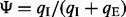 , where
  and
and  are the estimated abundance levels of two isoforms including and excluding the test exon, respectively, as illustrated in Supplementary Figure S8. We calculate the Ψ-values using both the ‘direct’ method and the above method based on isoform abundance levels estimated by our CEM algorithm and correlate the results with the Ψ-values calculated by qRT–PCR experiments in Table 3.
Table 3.
The R2-value and regression coefficient between the exon inclusion values calculated by RNA-Seq and qRT–PCR analyses
| Dataset | CTRL |
KD |
||
|---|---|---|---|---|
| Metric | Direct | CEM | Direct | CEM |
| R2 | 0.81 | 0.86 | 0.84 | 0.93 |
| Regression | 0.64x + 0.3 | 0.80x + 0.5 | 0.84x + 0.1 | 0.94x + 0.1 |
Table 3 shows a significantly improved correlation using the isoform abundance method based on CEM over the ‘direct’ method. The CEM algorithm achieves higher R2-values on both CTRL and KD datasets, and the regression slope ( ) on the KD dataset shows that the Ψ-values obtained by CEM are quite consistent with the qRT–PCR data.
4 CONCLUSIONS AND DISCUSSION
Biases in RNA-Seq data are difficult to deal with because they affect both transcriptome assembly and isoform abundance estimation. The current literature focuses on correcting biases for isoform abundance estimation, but little has been done for transcriptome assembly. In this article, we present a quasi-multinomial distribution-based statistical framework and component elimination EM algorithm for both transcriptome assembly and isoform abundance estimation from biased RNA-Seq data. Biases are captured by a single parameter  in the quasi-multinomial model, and the component elimination EM algorithm ensures that good interpretation (or sparsity) is achieved in transcriptome assembly.
Both simulated and real data experiments reveal interesting effects of different biases. Although the precision and sensitivity of a method in transcriptome assembly are affected by both positional and mappability biases, the recovery of isoforms/genes with different abundance levels are affected differently. While mappability biases reduce the sensitivity and precision for all genes, positional biases have a negative effect mainly on lowly or moderately expressed genes. A comparison between our CEM algorithm and the other methods in the literature shows that for highly expressed isoforms, our algorithm achieves higher sensitivity and precision in assembly. Also, our algorithm shows a higher accuracy in isoform abundance estimation (validated by MAQC gene expression level measurements).
Funding: The NIH R01 grant (AI078885).
Conflict of Interest: none declared.
Supplementary Material
REFERENCES
- Alter MD, et al. Variation in the large-scale organization of gene expression levels in the hippocampus relates to stable epigenetic variability in behavior. PLoS One. 2008;3:e3344. doi: 10.1371/journal.pone.0003344. [DOI] [PMC free article] [PubMed] [Google Scholar]
- Au KF, et al. Detection of splice junctions from paired-end RNA-seq data by SpliceMap. Nucleic Acids Res. 2010;38:4570–4578. doi: 10.1093/nar/gkq211. [DOI] [PMC free article] [PubMed] [Google Scholar]
- Bengtsson M, et al. Gene expression profiling in single cells from the pancreatic islets of Langerhans reveals lognormal distribution of mRNA levels. Genome Res. 2005;15:1388–1392. doi: 10.1101/gr.3820805. [DOI] [PMC free article] [PubMed] [Google Scholar]
- Bicego M, et al. Proceedings of the 14th International Conference on Image Analysis and Processing. 2007. Sparseness achievement in Hidden Markov Models. ICIAP'07, p. 67–72, IEEE Computer Society, Washington, DC, USA. [Google Scholar]
- Birol I, et al. De novo transcriptome assembly with abyss. Bioinformatics. 2009;25:2872–2877. doi: 10.1093/bioinformatics/btp367. [DOI] [PubMed] [Google Scholar]
- Consul PC, Jain GC. A generalization of the Poisson distribution. Technometrics. 1973;15:791–799. [Google Scholar]
- Consul PC, Mittal SP. Some discrete multinomial probability models with predetermined strategy. Biometrical J. 1977;19:161–173. [Google Scholar]
- Dempster AP, et al. Maximum likelihood from incomplete data via the EM algorithm. J. R. Stat. Soc. Ser. B (Methodological) 1977;39:1–38. [Google Scholar]
- Dohm JC, et al. Substantial biases in ultra-short read data sets from high-throughput DNA sequencing. Nucleic Acids Res. 2008;36:e105. doi: 10.1093/nar/gkn425. [DOI] [PMC free article] [PubMed] [Google Scholar]
- Feng J, et al. Inference of isoforms from short sequence reads. In: Berger B, editor. Research in Computational Molecular Biology, Vol. 6044 of Lecture Notes in Computer Science. Berlin: Springer; 2010. pp. 138–157. [Google Scholar]
- Figueiredo MAF, Jain AK. Unsupervised learning of finite mixture models. IEEE Trans. Pattern Anal. Mach. Intell. 2002;24:381–396. [Google Scholar]
- Fujita PA, et al. The UCSC Genome Browser database: update 2011. Nucleic Acids Res. 2011;39(Suppl. 1):D876–D882. doi: 10.1093/nar/gkq963. [DOI] [PMC free article] [PubMed] [Google Scholar]
- Grabherr MG, et al. Full-length transcriptome assembly from RNA-Seq data without a reference genome. Nat. Biotechnol. 2011;29:644–652. doi: 10.1038/nbt.1883. [DOI] [PMC free article] [PubMed] [Google Scholar]
- Guttman M, et al. Ab initio reconstruction of cell type-specific transcriptomes in mouse reveals the conserved multi-exonic structure of lincrnas. Nat. Biotechnol. 2010;28:503–510. doi: 10.1038/nbt.1633. [DOI] [PMC free article] [PubMed] [Google Scholar]
- Hansen KD, et al. Biases in Illumina transcriptome sequencing caused by random hexamer priming. Nucleic Acids Res. 2010;38:e131. doi: 10.1093/nar/gkq224. [DOI] [PMC free article] [PubMed] [Google Scholar]
- Hastie T, et al. The Elements of Statistical Learning: Data Mining, Inference, and Prediction, Chapter 3. Springer, New York; 2009. [Google Scholar]
- Howard B, Heber S. Towards reliable isoform quantification using RNA-SEQ data. BMC Bioinformatics. 2010;11(Suppl. 3):S6. doi: 10.1186/1471-2105-11-S3-S6. [DOI] [PMC free article] [PubMed] [Google Scholar]
- Hsu F, et al. The UCSC known genes. Bioinformatics. 2006;22:1036–1046. doi: 10.1093/bioinformatics/btl048. [DOI] [PubMed] [Google Scholar]
- Jiang H, Wong WH. Statistical inferences for isoform expression in RNA-seq. Bioinformatics. 2009;25:1026–1032. doi: 10.1093/bioinformatics/btp113. [DOI] [PMC free article] [PubMed] [Google Scholar]
- Langmead B, et al. Ultrafast and memory-efficient alignment of short DNA sequences to the human genome. Genome Biol. 2009;10:R25. doi: 10.1186/gb-2009-10-3-r25. [DOI] [PMC free article] [PubMed] [Google Scholar]
- Langmead B, et al. Cloud-scale RNA-sequencing differential expression analysis with Myrna. Genome Biol. 2010;11:R83. doi: 10.1186/gb-2010-11-8-r83. [DOI] [PMC free article] [PubMed] [Google Scholar]
- Lee S, et al. Accurate quantification of transcriptome from RNA-Seq data by effective length normalization. Nucleic Acids Res. 2010;39:e9. doi: 10.1093/nar/gkq1015. [DOI] [PMC free article] [PubMed] [Google Scholar]
- Li B, Dewey C. RSEM: accurate transcript quantification from RNA-Seq data with or without a reference genome. BMC Bioinformatics. 2011;12:323. doi: 10.1186/1471-2105-12-323. [DOI] [PMC free article] [PubMed] [Google Scholar]
- Li B, et al. RNA-Seq gene expression estimation with read mapping uncertainty. Bioinformatics. 2010a;26:493–500. doi: 10.1093/bioinformatics/btp692. [DOI] [PMC free article] [PubMed] [Google Scholar]
- Li J, et al. Modeling non-uniformity in short-read rates in RNA-Seq data. Genome Biol. 2010b;11:R50. doi: 10.1186/gb-2010-11-5-r50. [DOI] [PMC free article] [PubMed] [Google Scholar]
- Li JJ, et al. Sparse linear modeling of next-generation mRNA sequencing (RNA-Seq) data for isoform discovery and abundance estimation. Proc. Natl Acad. Sci. USA. 2011a;108:19867–19872. doi: 10.1073/pnas.1113972108. [DOI] [PMC free article] [PubMed] [Google Scholar]
- Li W, et al. IsoLasso: a LASSO regression approach to RNA-Seq based transcriptome assembly. In: Bafna V, Sahinalp S, editors. Research in Computational Molecular Biology, Vol. 6577 of Lecture Notes in Computer Science, Chapter 18. Berlin: Springer; 2011b. pp. 168–188. [DOI] [PMC free article] [PubMed] [Google Scholar]
- MAQC Consortium The MicroArray Quality Control (MAQC) project shows inter- and intraplatform reproducibility of gene expression measurements. Nat. Biotechnol. 2006;24:1151–1161. doi: 10.1038/nbt1239. [DOI] [PMC free article] [PubMed] [Google Scholar]
- Mortazavi A, et al. Mapping and quantifying mammalian transcriptomes by RNA-Seq. Nat. Methods. 2008;5:621–628. doi: 10.1038/nmeth.1226. [DOI] [PubMed] [Google Scholar]
- Nicolae M, et al. Estimation of alternative splicing isoform frequencies from RNA-seq data. In: Moulton V, Singh M, editors. Algorithms in Bioinformatics, Vol. 6293 of Lecture Notes in Computer Science. Berlin: Springer; 2010. pp. 202–214. [Google Scholar]
- Pan Q, et al. Revealing global regulatory features of mammalian alternative splicing using a quantitative microarray platform. Mol. Cell. 2004;16:929–941. doi: 10.1016/j.molcel.2004.12.004. [DOI] [PubMed] [Google Scholar]
- Paşaniuc B, et al. Accurate estimation of expression levels of homologous genes in RNA-seq experiments. In: Berger B, editor. Research in Computational Molecular Biology, Vol. 6044 of Lecture Notes in Computer Science, Chapter 26. Berlin: Springer; 2010. pp. 397–409. [DOI] [PubMed] [Google Scholar]
- Peng Y, et al. T-IDBA: a de novo iterative de Bruijn graph assembler for transcriptome. In: Bafna V, Sahinalp S, editors. Research in Computational Molecular Biology, Vol. 6577 of Lecture Notes in Computer Science, Chapter 31. Berlin: Springer; 2011. pp. 337–338. [Google Scholar]
- Richard H, et al. Prediction of alternative isoforms from exon expression levels in RNA-Seq experiments. Nucleic Acids Res. 2010;38:e112. doi: 10.1093/nar/gkq041. [DOI] [PMC free article] [PubMed] [Google Scholar]
- Roberts A, et al. Improving RNA-Seq expression estimates by correcting for fragment bias. Genome Biol. 2011;12:R22. doi: 10.1186/gb-2011-12-3-r22. [DOI] [PMC free article] [PubMed] [Google Scholar]
- Rozowsky J, et al. PeakSeq enables systematic scoring of ChIP-seq experiments relative to controls. Nat. Biotechnol. 2009;27:66–75. doi: 10.1038/nbt.1518. [DOI] [PMC free article] [PubMed] [Google Scholar]
- Salzman J, et al. Statistical modeling of RNA-Seq data. Stat. Sci. 2011;26:62–83. doi: 10.1214/10-STS343. [DOI] [PMC free article] [PubMed] [Google Scholar]
- Schwartz S, et al. Detection and removal of biases in the analysis of next-generation sequencing reads. PLoS One. 2011;6:e16685. doi: 10.1371/journal.pone.0016685. [DOI] [PMC free article] [PubMed] [Google Scholar]
- Srivastava S, Chen L. A two-parameter generalized Poisson model to improve the analysis of RNA-seq data. Nucleic Acids Res. 2010;38:e170. doi: 10.1093/nar/gkq670. [DOI] [PMC free article] [PubMed] [Google Scholar]
- Tibshirani R. Regression shrinkage and selection via the lasso. J. R. Stat. Soc. Ser. B (Methodological) 1996;58:267–288. [Google Scholar]
- Trapnell C, et al. Tophat: discovering splice junctions with RNA-seq. Bioinformatics. 2009;25:1105–1111. doi: 10.1093/bioinformatics/btp120. [DOI] [PMC free article] [PubMed] [Google Scholar]
- Trapnell C, et al. Transcript assembly and quantification by RNA-seq reveals unannotated transcripts and isoform switching during cell differentiation. Nat. Biotechnol. 2010;28:511–515. doi: 10.1038/nbt.1621. [DOI] [PMC free article] [PubMed] [Google Scholar]
- Wan L, et al. Modeling RNA degradation for RNA-Seq with applications. Biostatistics. 2012;13:734–747. doi: 10.1093/biostatistics/kxs001. [DOI] [PMC free article] [PubMed] [Google Scholar]
- Wang ET, et al. Alternative isoform regulation in human tissue transcriptomes. Nature. 2008;456:470–476. doi: 10.1038/nature07509. [DOI] [PMC free article] [PubMed] [Google Scholar]
- Wang Z, et al. RNA-Seq: a revolutionary tool for transcriptomics. Nat. Rev. Genet. 2009;10:57–63. doi: 10.1038/nrg2484. [DOI] [PMC free article] [PubMed] [Google Scholar]
- Wu Z, et al. Using non-uniform read distribution models to improve isoform expression inference in RNA-Seq. Bioinformatics. 2011;27:502–508. doi: 10.1093/bioinformatics/btq696. [DOI] [PubMed] [Google Scholar]
- Xiao X, et al. Splice site strength-dependent activity and genetic buffering by poly-G runs. Nat. Struct. Mol. Biol. 2009;16:1094–1100. doi: 10.1038/nsmb.1661. [DOI] [PMC free article] [PubMed] [Google Scholar]
- Ypma TJ. Historical development of the Newton–Raphson method. SIAM Rev. 1995;37:531–551. [Google Scholar]
Associated Data
This section collects any data citations, data availability statements, or supplementary materials included in this article.