Biphasic hemodynamic responses influence deactivation and may mask activation in block‐design fMRI paradigms

Abstract

A previous block‐design fMRI study revealed deactivation in the hippocampus in the transverse patterning task, specifically designed, on the basis of lesion literature, to engage hippocampal information processing. In the current study, a mixed block/event‐related design was used to determine the temporal nature of the signal change leading to the seemingly paradoxical deactivation. All positive activations in the hippocampal‐dependent condition, relative to a closely matched control task, were seen to result from positive BOLD transients in the typical 4–7 s poststimulus time range. However, most deactivations, including in the hippocampus and in other “default mode” regions commonly deactivated in cognitive tasks, were attributable to enhanced negative transient signals in a later time range, 10–12 s. This late hemodynamic transient was most pronounced in medial prefrontal cortex. In some regions, the hippocampal‐dependent condition enhanced both the early positive and late negative transients to approximately the same degree, resulting in no significant signal change when block analysis is used, despite very different event‐related responses. These results imply that delayed negative transients can play a role in determining the presence and sign of brain activation in block‐design studies, in which case an event‐related analysis can be more sensitive than a block analysis, even if the different conditions occur within blocks. In this case, default mode deactivations are timelocked to stimulus presentation as much as positive activations are, but in a later time range, suggesting a specific role of negative transient signals in task performance. Hum Brain Mapp, 2008. © 2007 Wiley‐Liss, Inc.

INTRODUCTION

Functional MRI experiments are commonly designed in one of two different ways: block‐design or event‐related. In a block design experiment, task conditions are held constant for a relatively long time (15–50 s is typical), and analysis is carried out using a boxcar shaped regressor function reflecting the timing of task conditions, usually convolved with a model of the hemodynamic response in order to account for the delay between neural activity and associated changes in blood flow. Block designs are similar to PET paradigms, which necessarily use long blocks because of the relatively poor temporal resolution of the technique. In fMRI, however, it is also possible to study hemodynamic changes at higher temporal resolution, using event‐related designs. Event‐related designs are desirable in many cases, as they allow closely‐spaced single trials to be classified into different conditions, based either on design or behavioral outcome, and are therefore more comparable to typical designs in reaction‐time based experimental psychology or ERP research.

Nonetheless, the block design has a number of advantages. First, a block design may be the only appropriate method for certain cognitive tasks that do not fall neatly into a single‐trial paradigm, such as listening to a continuous narrative or using a driving simulator. Second, a block design has much more statistical power than an event‐related experiment of the same length [Liu et al., 2001], and so it may be desirable to implement certain experiments as a block design even if they could conceivably be divided into single trials. However, comparisons between block and event‐related designs have generally been carried out under the assumption that the two yield largely equivalent information on the relative amount of neural activity involved in a particular process. Given that the hemodynamic responses to rapidly presented single trials have been observed to sum linearly [Boynton et al., 1996], or somewhat sublinearly with very short ISIs [Liu and Gao, 2000; Soltysik et al., 2004], block‐design activations are commonly regarded as a sum of evoked responses to single trials occurring within a block. However, few studies [Chee et al., 2003] have directly compared block and event‐related versions of the same task to evaluate this relationship. In the current study, we used a mixed block/event‐related design that allowed us to analyze the same data both ways, resulting in a direct comparison between the two modeling approaches. This comparison yielded some surprising dissociations: while robust positive and negative activations on the block level were indeed seen to arise from event‐related signals, the time courses of positive and negative transients were very different, with negative signal changes occurring at a later time relative to stimulus presentation. Furthermore, we observed several regions in which the hemodynamic responses in two conditions were very different from each other, but mutual cancellation of early positive and later negative transients resulted in no significant difference between the two conditions on the block level. These findings indicate that using the standard hemodynamic response function (HRF) in cognitive paradigms may be insufficient, and that empirically derived estimates of hemodynamic responses can reveal differences in brain activity that are undetectable in block analysis, even if the task does have a blocked structure.

The current study is a follow‐up to an earlier block‐design fMRI study by our group [Astur and Constable, 2004], which reported a somewhat surprising finding. Bilateral hippocampal deactivation was detected in a task specifically designed to engage the hippocampus, on the basis of human and animal lesion data. In this task, pairs of stimuli are presented, and in each pair, one stimulus is designated correct and one is designated incorrect. The subject must choose one stimulus as the correct one, and feedback is provided to teach the correct responses. To solve the problem, one must learn the following rule: A is correct when paired with B; B is correct when paired with C; and C is correct when paired with A. This problem, known as “transverse patterning,” [Spence, 1952] is identical to the game “Rock Paper Scissors,” in that each stimulus is ambiguous, but by attending to the relations between the stimuli, the problem can be solved. Hippocampal damage has been shown to severely disrupt performance of this task in rats [Alvarado and Rudy, 1995; Dusek and Eichenbaum, 1998; but see Bussey et al., 1998], monkeys [Alvarado et al., 2002], and humans [Reed and Squire, 1999; Rickard and Grafman, 1998], relative to a control condition in which the same stimuli are consistently designated as correct or incorrect regardless of their pairing. Hereafter, we refer to such a control condition as “elemental,” while the task condition involving the transverse patterning problem is referred to as “configural” (Fig. 1A,B).

Figure 1.

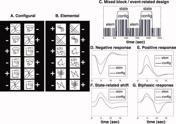
Task design and hypotheses. A: The stimuli and valences for the configural condition, which involved solving the transverse patterning problem. All 6 possible stimulus pairings within the condition are shown, with the correct answer marked with “+” and the incorrect with “−”. Only two pictures were shown at a time, as described in the text. In this condition, each picture is rewarded and non‐rewarded 50% of the time, depending on the picture with which it is paired. B: The elemental condition, which served as a control condition. In this condition, each picture is either rewarded or non‐rewarded 100% of the time, making the task not dependent on associative memory. C: Illustration of the mixed block‐event related design. Vertical bars of different heights represent the pseudo‐random times of occurrence of individual trials in the two conditions, while the solid line represents the timing of the configural condition block convolved with a simple hemodynamic regressor function, used to model sustained block‐level signal shifts. D: Hypothetical signal behavior under the item‐related hypothesis: negative responses larger in the configural condition. E: An alternative behavior also consistent with item‐related deactivation: positive responses larger in the elemental condition. F: Signal behavior consistent with state‐related deactivation: cognitive events occurring preferentially in the elemental condition but not timelocked to stimulus presentation result in the detection of a sustained signal offset. G: The unexpected result of the experiment: deactivation arises from a delayed negative transient signal.

The previous fMRI study of transverse patterning [Astur and Constable, 2004] employed a block design with three conditions: the configural version of the task, the elemental version, and a resting fixation condition used as a baseline. In the hippocampus, BOLD signal levels were lower during performance of the configural condition than in the elemental condition, and both were lower than signal levels during the fixation baseline. Noting that hippocampal signal levels have previously been observed to be relatively high during resting baseline conditions compared with other possible control tasks [Stark and Squire, 2001], the authors note the possibility that the apparent deactivations are due to the presence of more ongoing mental activity involving the hippocampus during the less attentionally demanding elemental and fixation conditions, as opposed to a genuine decrease in metabolic activity induced by the configural task. Interestingly, a similar explanation is often invoked for ubiquitous findings of task‐induced deactivation in a network of regions commonly known as the “default mode network” [Gusnard and Raichle, 2001], including medial prefrontal cortex, posterior midline cortex, and, according to some authors, the hippocampus as well [Greicius and Menon, 2004]. As the term “default mode” implies, several authors have theorized that these regions are involved in cognitive processes that are highly active in the absence of external attentional demands, and that difficult cognitive tasks require a reallocation of resources away from these processes to meet the demands of the tasks, thus decreasing the observable hemodynamic and metabolic signals in these areas [McKiernan et al., 2003; Raichle at al., 2001].

A careful consideration of the literature on task‐induced deactivation reveals that two slightly different scenarios involving default mode deactivation have been reported. In the remainder of this introductory section, we will lay out these two hypotheses, along with the separate predictions generated by each in an experiment designed to distinguish between them. In the first version, which we shall call “state‐related deactivation,” the cognitive processes implemented by default mode structures wax and wane independently of the task‐related processes, although they are somewhat less likely to occur when a subject is engaged in a highly demanding task, leading to deactivation. This is the kind of scenario implied by Stark and Squire [2001] in their examination of hippocampal signal levels in low‐demand baseline conditions. As the hippocampus is involved in retrieval of recent memories, which is a key feature of unrestrained spontaneous thought, it follows that a higher amount of spontaneous thought occurring during periods of lower external task demand would cause higher signal levels on average during that period. Empirical support for state‐related deactivation is demonstrated by Greicius and Menon [2004], who used Independent Component Analysis on fMRI data, finding that activity in default mode structures (including the hippocampus) exhibited coherent fluctuations that were temporally uncoupled from positive activations to visual and auditory stimuli, although activity in these regions tended to be higher during rest periods, leading to task‐induced deactivation on the block level only in some cases.

The second scenario, “item‐related deactivation,” involves signal decreases that are tightly coupled to increases elsewhere, with a specific temporal relationship to trials occurring within the task. Examples are found in event‐related fMRI studies that have shown negative hemodynamic responses timelocked to stimulus presentation events, which are modulated by cognitive factors. For instance, Daselaar et al. [2004] report greater event‐related deactivations in default mode regions in response to visual stimuli that are successfully encoded into long‐term memory, compared with those that are forgotten. Polli et al. [2005] noted a failure to deactivate default mode regions on error trials in a saccade task, compared with correct trials. Findings such as these imply that deactivations may play an important role in task performance, compared with the predictions of the state‐related hypothesis, in which signal decreases are viewed as a byproduct of essentially independent processes.

To determine which kind of temporal signal behavior was responsible for the observed deactivation in the transverse patterning task (both in the hippocampus and in other regions), we re‐designed the earlier version of the transverse patterning task [Astur and Constable, 2004] as a mixed block/event‐related study, as illustrated in Figure 1C. Individual trials are presented in blocks of each condition, with a jittered inter‐stimulus interval. In a mixed design study, models of the hemodynamic response to individual item presentations are used to detect item‐related signal changes, while the timecourse of block alternations (of a “boxcar” shape) is also convolved with a hemodynamic model in order to detect sustained state‐related changes simultaneously, through multiple regression [Erickson et al., 2005; Otten et al., 2002]. Because items of the same condition are grouped into blocks, the item‐related and state‐related regressors can be highly correlated with each other. Nonetheless, it is possible to estimate both effects simultaneously, especially if a jittered ISI is used [Otten et al., 2002]. However, successful dissociation of item‐related and state‐related effects depends on the accuracy of the hemodynamic model used, as item‐related signal changes that are not well‐modeled by the item‐related regressor may mistakenly be attributed to sustained state‐related shifts [Amaro and Barker, 2006]. In this study, we compare several methods for the analysis of a mixed‐design study such as this, demonstrating that a more flexible modeling strategy allows for the detection of item‐related effects that do not fit the standard hemodynamic model.

In Figure 1D–G, we sketch the behavior of the BOLD signal to be expected under the alternative explanations of task‐induced deactivation described above. Figure 1D shows a negative‐going hemodynamic response in both conditions, of a standard “canonical” shape consisting of a gamma density function and a second “undershoot” function peaking 6 s later of the same shape, opposite sign, and 1/6 the amplitude of the primary response (as is used in the SPM software). The negative response is larger in the configural condition, leading to deactivation on the block level. This kind of response is an example of item‐related deactivation, as the negative signal occurs with the same timing as positive signals elsewhere. Figure 1E demonstrates another form of item‐related signal behavior that can also lead to deactivation in the configural condition on the block level. In this case, both conditions elicit a positive hemodynamic response, which is larger in the elemental condition. Given that the previous study found that both task conditions tended to have lower signal levels than a fixation baseline condition [Astur and Constable, 2004], we would not expect to encounter this scenario in the current study, but we include it as a logical possibility. Figure 1F shows the signal behavior associated with state‐related deactivation decoupled to task events. In this case, positive signal deflections occurring preferentially in the elemental condition result in the detection of a sustained offset in signal level between the two conditions, reflected by the different baselines in the two conditions. It is important to note that such a scenario does not actually require a sustained low‐frequency offset in signal level. Rather, it merely requires that the signal fluctuations associated with task‐independent cognitive events do not occur in a manner precisely timelocked to the presentation of task‐stimuli. Since these “randomly” occurring events cannot be modeled accurately, the resulting average signal difference should be distributed throughout peristimulus time.

In Figure 1G, we present a sketch of a different form of signal behavior leading to task‐induced deactivation. In this scenario, the hemodynamic response is biphasic, with a small initial increase followed by a larger decrease, or “undershoot.” Here, a larger undershoot in the configural condition leads to a lower average signal on the block level, even though the initial positive response is also larger in that condition. Although this behavior was not originally hypothesized when the study was designed, timecourses such as these were observed in several brain regions. In deactivated regions, the negative signal change in the configural condition was mainly attributable to a later negative transient peaking several seconds after the positive response, while in other regions the configural condition evoked both a larger initial positive response and a larger negative transient in a later timerange, leading to mutual cancellation and no net signal change on the block level. The presence of a late‐peaking event‐related negative transient is, to our knowledge, a novel finding. However, the detection of this transient depended on specialized statistical methods that were motivated by the specific hypotheses investigated in this study. Our results suggest that late‐peaking negative transients may be present in numerous tasks, and can lead to misleading results in block and mixed block/event‐related studies in which the variable nature of the hemodynamic response is not considered.

METHODS

Subjects

A total of 17 participants were recruited from the Yale University Community, ranging from 22‐ to 28‐years of age. All subjects gave informed consent, had normal or corrected vision, and were paid for their participation. The study protocol was approved by the Yale University Human Investigation Committee.

Behavioral Task

Two different conditions were contrasted in the behavioral task. In the configural condition, participants were exposed to the transverse patterning problem (A+ vs. B−; B+ vs. C−; C+ vs. A−), and in the elemental condition, participants were exposed to a control problem (U+ vs. V−; W+ vs. X−; Y+ vs. Z−). Note that no relational solution is required for the control problem, and that this problem can be solved by individuals with hippocampal damage [Alvarado and Rudy, 1992; Reed and Squire, 1999; Rickard and Grafman, 1998]. Subjects were told that they would see two pictures, that they were to select which one is the “winner,” and that the computer would give auditory feedback about whether or not their choices were correct. To choose a stimulus, the participant pushed one of two buttons corresponding to the presentation side of the image (left or right side). Correct responses were followed immediately by a pleasant chime, while incorrect responses were followed by a brief buzzer sound. Auditory feedback was used throughout the experiment to maintain a high level of accuracy. Response time and accuracy were recorded by the computer. The paradigm was slightly modified from the previous block‐design study in order to accommodate a mixed block/event‐related analysis. Stimuli were presented for 2,500 ms, and the interstimulus interval (ISI) varied pseudo‐randomly from 3,100 to 7,750 ms (integer multiples of the TR). Mathematical simulations were performed to select a set of interstimulus‐intervals affording optimal statistical efficiency for linear regression of overlapping hemodynamic responses [Dale, 1999]. The intervals selected were based on tradeoffs between increasing statistical power and maintaining the block‐like structure of the task (both of which encourage a shorter ISI), and avoiding nonlinearities in the BOLD response, which encourages a longer ISI. While some studies have suggested that nonlinearities are present in overlapping hemodynamic responses in certain brain regions with ISIs as short as 3 s, in every reported case the form of this nonlinearity has been a change in the amplitude or width of the response, not a fundamental alteration of its shape [Boynton et al., 1996; Liu and Gao, 2000; Soltysik et al., 2004]. Therefore, there is no evidence to suggest that the biphasic nature of the hemodynamic responses observed in this study is an artifact attributable to short ISIs. Furthermore, the two conditions were completely balanced, avoiding potential artifactual activation differences attributable to nonlinear effects [Wager et al., 2005]. Stimuli were presented in four alternating blocks of 12 of each condition, for 96 trials per run. Runs alternately started with the configural or elemental condition. Each subject performed five runs during fMRI acquisition.

Training

In the previous fMRI study of transverse patterning [Astur and Constable, 2004], subjects learned the correct responses through auditory feedback during the fMRI session. Therefore, the acquired data comprised a mixture of learning stages, from initial guessing to final skilled asymptotic performance. Because similar results were obtained from analysis of asymptotic‐stage data alone, we chose to focus exclusively on that stage in this study by pre‐training the subjects up to asymptotic performance. Subjects were trained immediately prior to the fMRI session, using a staged training paradigm that has been shown to be optimal for teaching the transverse patterning task to humans, while generally ensuring that subjects adapt a configural strategy for solving it [Astur and Sutherland, 1998]. During the training period, stimuli were presented once every 4 s, and remained on the screen for 3 s, which was the maximum time allowed for response and feedback. Subjects were trained on one pair from each set (configural and elemental) at a time, until all six pairs had been encountered. Subjects then did a set of all stimuli in random order, but blocked into sets of six at a time from each condition. At this point, most subjects were at nearly 100% performance on the elemental condition but not on the configural condition. We then discussed the logical structure of the configural condition explicitly with subjects, using the rock‐paper‐scissors analogy. Subjects were then given extra rounds of practice on the configural condition alone, until they reached near‐perfect performance. All subjects reached this point within 20 min.

FMRI Acquisition

FMRI was performed on a 3‐Tesla Siemens Trio system. Foam padding and tape were used to minimize head movement. Stimuli were projected onto a mirror attached to the head coil above the subject's face. Subjects' responses were registered using a fiber‐optic button box (Current Designs, Philadelphia, PA) and feedback auditory stimuli were delivered through MRI‐compatible headphones (Resonance Technologies, Northridge, CA). After localizer scans, 25 axial slices were defined covering the whole brain, parallel to the line between the anterior and posterior commissures. In this orientation, we first acquired a T1‐weighted anatomic image. Next, subjects performed the cognitive task during acquisition of functional EPI images (64 × 64 matrix, FOV 220 mm, TE 30 ms, TR 1,550 ms, in‐plane voxel size 3.4 × 3.4 mm², slice thickness 6 mm, no skip, interleaved ascending acquisition, α = 80°), in the same AC‐PC aligned 25‐slice geometry. After completion of the cognitive task, a high‐resolution 3D MPRAGE anatomical image was acquired.

FMRI Analysis

FMRI preprocessing and statistical analysis was conducted with AFNI software (http://afni.nimh.nih.gov/afni/), supplemented by programs written locally in MATLAB 6.5 (Mathworks, Natick, MA). EPI images were skull‐stripped (Brain Extraction Tool, http://www.fmrib.ox.ac.uk/fsl/), corrected for differences in slice‐timing, and motion‐corrected with the AFNI program 3dvolreg, which uses a weighted least squares rigid‐body registration algorithm [Cox and Jesmanowicz, 1999]. Next, images were spatially smoothed with an 8‐mm FWHM Gaussian kernel, and normalized so that the mean of every voxel's time course in each run was 100, allowing subsequent regression parameter estimates to be interpretable as percent signal change. Statistical analysis was carried out on the single‐subject level through multiple linear regressions using several different approaches, which are described below. Possible confounding effects of low‐frequency signal drifts and motion artifacts were mitigated by including additional covariates in the regression model, namely a third‐order Legendre polynomial series for drifts, and the six rigid‐body motion parameters estimated for each time point in the motion‐correction procedure.

Functional images resulting from within‐subject statistical analysis were warped into a reference space (the “Colin brain,” http://www.mrc-cbu.cam.ac.uk, skull‐stripped locally) with MNI coordinates, using a three‐step transformation: a 6‐parameter rigid transformation from the EPI image to the axial anatomical, a 6‐parameter rigid transformation from the axial anatomical to the high‐resolution MPRAGE image, and a 12‐parameter affine plus nonlinear grid‐based transform [Papademetris et al., 2004] from the individual subject's skull‐stripped MPRAGE to the reference brain, implemented with in‐house software.

Multisubject activation maps were created by submitting percent‐signal change values at each voxel to a one‐sample t‐test across subjects (except for the ANOVA tests, see below), thus treating subjects as a random effect [Penny and Holmes, 2004]. For correction of multiple comparisons, all activation maps were thresholded with a voxel‐wise threshold of P < 0.01, and a cluster size threshold of 2.16 mL, determined by Monte Carlo simulations (the AFNI program Alphasim), for a corrected family‐wise error rate of P < 0.05 on the cluster level [Forman et al., 1995]. The use of a cluster‐size threshold such as this favors the detection of large clusters rather than focal areas exhibiting the largest effect sizes. As a result, some very small but highly significant activations may go undetected. As we were not interested in making fine‐grained anatomical distinctions in this study, but rather in exploring the temporal signal behavior that gives rise to block design outcomes of positive and negative activation, we opted for this approach to avoid restricting the analysis to only the most highly activated areas.

Traditional Block Design Analysis

To distinguish between state‐related and item‐related signal changes, we used several different modeling strategies on the same data. A major goal of this study is to compare the relative strengths of different approaches that are commonly available, emphasizing the different conclusions that result from them and the reasons for the discrepancies. First, we used a traditional block‐design analysis, ignoring the fact that the task was comprised of individual trials. This analysis represents a straightforward replication of the previous block‐design study [Astur and Constable, 2004]. One regressor for average signal differences in the configural condition compared with the elemental condition was constructed by convolving the block timecourse of the configural condition with a standard HRF in the shape of a gamma density, which is a commonly used default in AFNI software (a similar model is used in SPM and other packages). This model is as follows:

(1)

where s is the signal to be modeled, t is post‐stimulus time, b and c are parameters derived from empirical observations and set here to 8.6 and 0.547, respectively [Cohen, 1997], and A is the amplitude parameter whose value is to be estimated in the regression procedure. In this analysis, the block time course of the configural condition was modeled, while the elemental blocks served as the baseline.

Item‐Related Analysis

In this analysis, the same hemodynamic model was used as in the traditional block‐design analysis, but rather than convolving the entire boxcar time course, only the specific onset times of individual items were used. In this case, item onsets from both conditions, configural and elemental, were convolved with hemodynamic regressors, while the interstimulus intervals served as the baseline. The contrast between the two conditions was computed by subtracting the regression coefficients for the two conditions, configural minus elemental.

Mixed Block/Event‐Related Analysis

To determine whether the observed positive and negative activations arose from state‐related or item‐related effects, we adopted a procedure used in a previous mixed‐design study with similar goals [Otten et al., 2002]. In this approach, both state and item effects are modeled with a standard HRF. If stimulus presentation is perfectly periodic, it is impossible to model both effects separately, because the modeled response to items reaches a steady state and is thus perfectly correlated with the block regressor. A jittered ISI allows item and state related effects to be separated, while maintaining the block‐like structure of the task. This approach is attractive in its simplicity, as it allows contrasts between conditions to be computed on the basis of a single regression coefficient for each condition [Friston et al., 1998]. In this case, item‐related effects were calculated by subtracting the hemodynamic response coefficients, configural minus elemental, while state‐related effects were represented by the single coefficient of the block regressor. A drawback to this approach, however, is that results may be misleading if the actual hemodynamic response to items is not a good match for the model function. Item‐related signal changes whose temporal relationship to the stimuli differ greatly from the model may contribute instead to the block regressor, giving the false impression that activation is a sustained shift rather than a stimulus‐locked transient. We will demonstrate below that this is indeed the case in the current study.

Finite Impulse Response Model Analysis

The use of a prespecified hemodynamic model is the most common approach to analysis of event‐related fMRI. A chief advantage of this method is that it produces a single regression parameter for each subject, which is easily submitted to a second‐level multisubject statistical analysis. Unfortunately, results can be misleading if the actual shape of the hemodynamic response is not a good match for the model. An alternative procedure is to use Finite Impulse Response (FIR) models, in which the shape of the hemodynamic response is empirically estimated by modeling each trial as a series of delta functions at several time delays relative to stimulus presentation. (For mathematical details, see Miezin et al., 2000]. With widely spaced trials, this is essentially equivalent to averaging the BOLD signal timelocked to stimulus presentation, but it also allows similar estimates to be made when trials are closely spaced with overlapping hemodynamic responses.

The condition‐specific stimulus‐locked impulse response functions (IRF) for each voxel were estimated at 12 timepoints, from 0 to 17.05 s, in integer multiples of the TR, using the AFNI program 3dDeconvolve. The resulting 24 parameter estimates (2 conditions × 12 timepoints) were then used for two purposes. The first was to generate plots of the empirically derived HRFs in specific regions of interest, selected on the basis of the previous block design and mixed design analyses. Timecourses for each condition and voxel were averaged across subjects. Visual inspection of the resulting plots makes it possible to judge whether the condition differences on the block level arise from sustained offsets or from specific transient signals timelocked to trial onset, even if the transient signals are not a good match for a canonical hemodynamic response model, as illustrated in Figure 1D–G. For the plots of timecourses, locations were manually chosen from activated regions, and signals within a 1 mL spherical ROI (125 voxels) were averaged.

A second use of the FIR estimates was to produce whole‐brain maps of brain activation. This is not as straightforward as it is in conventional model‐based analysis, which may explain why FIR models are not as commonly used. While an F‐test may be used to determine if the FIR timecourses of two conditions differ significantly within a single subject, conventional forms of multisubject analysis require the generation of a signed quantity for each subject to be submitted to a second‐level statistical procedure. When multiple quantities are involved, as is the case with an FIR series of timepoints, a useful approach is to enter the estimated timecourses into a repeated‐measures Analysis of Variance (ANOVA). This approach has been used extensively on timecourses estimated from specific regions of interest [Cato et al., 2004; Davachi and Wagner, 2002], but has not commonly been used to construct whole‐brain statistical maps. Thus, the IRF of each voxel, condition, and subject were entered into a voxel‐wise repeated measures ANOVA, with subject as a random factor and condition (configural or elemental) and time (12 timepoints) as fixed within‐subject factors. The tests of interest are for a main effect of condition and a condition‐by‐time interaction.

A main effect of condition indicates that the average signal level across the whole response is higher in one condition. As there were only two conditions, the F‐test from the ANOVA is equivalent to a paired t‐test across subjects on the sum of the entire hemodynamic response (or, equivalently, the area under the curve). Therefore, if the FIR model is adequately fitting the data, the brain map for main effect of condition should be almost identical to the traditional block‐design analysis. A main effect of condition, therefore, is compatible with either a sustained shift or a large timelocked transient.

More importantly, a test for a condition‐by‐time interaction identifies areas in which the difference between conditions is time‐dependent, and therefore attributable to event‐related transient effects of any shape. Because time measurements are serially correlated, they may violate the sphericity assumption in univariate repeated‐measures ANOVA, resulting in misleadingly low P‐values and false positives. Typically, a data‐driven correction procedure [Greenhouse and Geiser, 1959] is used to calculate a reduced number of degrees of freedom for valid p‐values. In fMRI, such a procedure would require a different number of degrees of freedom at each voxel, which most software is not equipped to deal with. As an alternative, we used lower‐bound correction [Greenhouse and Geiser, 1959], which produces a valid test with uniform degrees of freedom, at the cost of extreme conservativeness. Therefore, the resulting brain map identifies regions with the most robust transient effects but may miss regions with more modest but significant effects. However, the identification of additional areas would not change the basic conclusions of the current study. The correction was done by modifying the degrees of freedom associated with the time effect and condition‐by‐time interaction, according to the procedure described in Baron and Li [2004].

RESULTS

Behavioral

As expected, the configural condition was considerably more difficult than the elemental condition, as determined by measures of reaction time and accuracy, even though subjects were given extensive training on the configural condition in order to bring performance well above 90%. Average reaction times were: Configural, 1,067 ms, SEM 28; Elemental, 772 ms, SEM 19 (paired t‐test, t(16) = 14.01, P < 10⁻⁹). Average percent correct scores were: Configural, 96.88%; Elemental, 98.94% (t(16) = 4.21, P < 0.001). In informal debriefing, most subjects reported that the elemental condition became almost automatic and effortless, whereas the configural condition, while not overly difficult, required constant attention and conscious effortful decision making, even after much practice. Subjects reported using an overt declarative strategy in the configural condition, such as assigning verbal labels to the stimuli and recalling rules (e.g. “circles beat squares, squares beat spaghetti”).

Traditional Block Design Analysis

The first analysis used a simple block‐design model, simply to identify average differences between the two conditions regardless of the transient behavior of the signal. The whole‐brain map resulting from this analysis is presented in Figure 2A. In this and all subsequent t‐test analyses, the subtraction is [configural minus elemental], with positive values (config > elem) plotted in red on brain maps and negative values (elem > config) plotted in blue. Signal levels in much of the brain were significantly different in the two conditions (Fig. 2A). Positive activations were detected in bilateral inferior frontal gyri, bilateral parietal cortex, and in the basal ganglia, all of which are regions implicated in a broad range of memory retrieval tasks [Poldrack and Rodriguez, 2004; Rugg et al., 2002]. Interestingly, a larger portion of the brain exhibited deactivation, i.e. lower signal during the more difficult configural condition. Deactivated regions included components of the so‐called “default mode” network [Greicius and Menon, 2004; Raichle et al., 2001], including anterior and posterior midline and cingulate cortices, lateral parietal regions, and, as previously reported [Astur and Constable, 2004], the hippocampus.

Figure 2.

Block, state, and item‐related effects. A: The whole‐brain activation map produced by using a simple block‐design analysis, comparing average signal levels in configural vs. elemental blocks. Maps are scaled to maximum percent signal change. B: Configural minus elemental map, using a γ‐function model HRF convolved with the exact timings of stimulus presentation, rather than the overall block timing. C: Item‐related activity in the mixed‐design analysis, contrasting the hemodynamic response (a single γ‐function model) in the configural vs. elemental condition. D: State‐related activity in the mixed‐design analysis, showing areas in which activation differences between blocks were not fit by the item‐related model, but by the sustained regressor. E: Main effect of condition in the FIR‐based ANOVA analysis, showing that the sum of the FIR regressors is equivalent to the block‐design contrast in panel D. F: Condition‐by‐time interaction map from the ANOVA analysis, showing areas in which the signal difference between conditions varies maximally with time, respective to stimulus presentation. This analysis is the most sensitive to biphasic responses.

Item‐Related Analysis

In this analysis, the precise onset times of individual stimuli were used to construct the modeled hemodynamic response, rather than a simple boxcar shape reflecting the alternation of blocks. Because stimuli of the same condition are grouped into the same block, and generate overlapping hemodynamic responses, the resulting regressors are highly similar to those that are used in the traditional block design. Nonetheless, this design is potentially more sensitive to transient item‐related signal changes that may not be reliably detected on the coarser level of the block. The resulting activation map, presented in Figure 2B, closely resembles the block‐design map in Figure 2A, as expected. However, there are some systematic differences. The item‐related analysis appears somewhat more sensitive to positive activation, as a significant cluster in the dorsal anterior cingulate cortex is detected, which was not evident in the block subtraction. On the other hand, sensitivity to deactivations is reduced, as the blue regions of the map are smaller in extent, and some regions of deactivation, such as in the bilateral medial temporal lobes, are not detected in the item‐related analysis. This pattern of dissociation suggests that positive and negative signal changes have a different timecourse, with positive activations conforming more closely to the standard model of the hemodynamic response, while deactivations are attributable to signal changes with different temporal behavior. This observation is confirmed and explained by further analyses presented below.

Mixed Block/Event‐Related Analysis

Next, we used a mixed block/event‐related analysis, with standard hemodynamic models for both item and state‐related effects. Results of the item and state‐related contrasts are presented in Figure 2C,D, respectively. At first glance, these maps support a complete dissociation between positive and negative signal changes: the item‐related effects are exclusively positive, indicating a greater stimulus‐locked response in the configural condition, while the state‐related effects are exclusively negative, suggesting that deactivation arises from sustained signal shifts, temporally uncoupled from stimulus presentation. However, subsequent analyses demonstrate that this is not the case.

A closer look at Figure 2A,C,D reveals some puzzling discrepancies. If the mixed block/event‐related approach is adequately modeling the data, one would expect the activations in Figure 2A (the pure block design) to be a superset of those in 2C,D (the item and state‐related activations). While the state‐related deactivation is a good match for the block‐design deactivations, the item‐related positive activations do not correspond well to the regions of positive activation in the pure block design map. The extensive lateral parietal activations seen in the block design map do not show up in the item‐related analysis, while the item‐related analysis detects several activations that are not present in the block design map, including the dorsal anterior cingulate, the precuneus, and the thalamus. If there is a greater transient response to configural trials in these regions, it is strange that they do not sum up to a higher average signal level on the block level. This is a surprising dissociation between block and event‐related analysis of the same data. These apparent discrepancies were resolved upon inspection of the signal timecourses obtained through the use of the FIR modeling procedure.

FIR Model Analysis

While the mixed analysis described above clearly indicates that positive and negative signal changes have a different temporal relationship to the stimuli, two major questions remain about the proper interpretation of that dissociation. First, the deactivations may truly be sustained shifts in the average signal level occurring over the block, or they could instead be driven by item‐related effects that are not well modeled by the standard HRF. Second, why are some areas activated positively in the item‐related analysis but not on the average block level? To answer both these questions, we used FIR models to empirically estimate the shape of the hemodynamic response in each condition, and both of these issues turned out to relate to the same phenomenon: a later negative transient, or undershoot, in the hemodynamic response.

Voxel‐wise repeated measures ANOVA was used to detect areas exhibiting a main effect of condition, which should be nearly equivalent to the standard block‐design analysis, and a condition‐by‐time interaction, which would indicate strong transient signals that differ between conditions. The main effect of condition map is displayed in Figure 2E, and as expected, closely resembles the block design map in 2A, which serves to validate the idea that the FIR model is successfully capturing the relevant signal changes. The interaction map is displayed in Figure 2F. This map is very similar to the item‐related analysis displayed in Figure 2C, although it additionally includes some of the left‐lateralized parietal region that was positively activated on the block level.

The fact that the FIR‐based ANOVA maps closely resemble those derived from canonical HRFs is reassuring, but the chief advantage of the FIR approach is not its ability to produce maps but rather the ability to examine the empirically estimated hemodynamic timecourses at specific locations. This is especially true for the current study, in which the apparent discrepancies between the block‐design and mixed‐design analyses may be resolved by observing the shape of the responses. Therefore, we selected regions of interest on the basis of the maps and plotted the average signals at these locations.

Timecourses of regions showing a main effect of condition (i.e. a block‐level signal difference) are displayed in Figure 3. In all of these ROIs, the difference between the activity integrated over the entire time range is highly significant (P < 0.001). Signals from the two largest regions of positive signal change in the configural condition, the left and right lateral parietal regions, are shown in Figure 3A,B. In both of these regions, it is clear that stimulus presentation induces a transient signal increase that is larger in the configural condition. The peak of this transient occurs at ∼6 s poststimulus, which is typical for an event‐related hemodynamic response. Positive signal changes, therefore, seem to be driven by item‐related processes, and not by sustained shifts, consistent with the results of the mixed‐design analysis.

Figure 3.

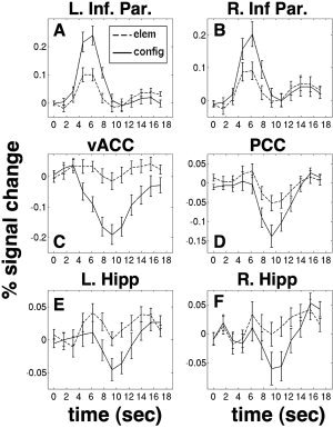
Timecourses of regions showing a main effect. A: Left inferior parietal lobe, MNI coordinates X = −34, Y = −56, Z = 44. This region was positively activated in the block‐design comparison, as a result of a hemodynamic transient peaking at about 6 s. Error bars represent standard error of the mean across subjects. B: Right inferior parietal lobe, (coords. 33, −60, 44), also positively activated. C: Ventral anterior cingulate cortex, (coords. 0, 43, 1), deactivated on the block level because of a later negative transient peaking at about 10 s. D: Posterior cingulate, (coords. 0, −36, 40), also deactivated due to a late transient. E: Left hippocampus, (coords. −32, −25, −16), deactivated. F: Right hippocampus (coords. 28, −29, −18), deactivated.

Timecourses of regions showing deactivation in the configural condition are shown next. Figure 3C displays the timecourse from the ventral anterior cingulate, which, along with the adjacent ventromedial prefrontal cortex, is one of the regions most consistently deactivated in cognitive tasks. Clearly, the signal differences in this region are also driven by a transient signal that is timelocked to stimulus presentation. However, it differs in shape from the standard event‐related response in that it is quite broad and peaks very late, around 10 s poststimulus. The fact that the first and last points on the estimated responses are nearly the same in the two conditions indicates that the deactivation in this region is not truly a sustained shift. Timecourses in the posterior cingulate, also commonly deactivated, are shown in Figure 3D. Again, the deactivation in the configural condition is seen to arise from a later negative transient, with a minimum signal level at ∼10 s poststimulus.

Because a major goal of this study was to evaluate the temporal behavior of the seemingly paradoxical hippocampal deactivation in this task, we also examined time courses in deactivated portions of the hippocampus. Signals from the left and right hippocampi are shown in Figure 3E,F, respectively. In both regions, the difference between conditions is again seen to arise primarily from a later negative transient in the hemodynamic response. In every deactivated region in which we looked (including others not shown here), the lower signal level in the configural condition is chiefly attributable to this late transient, as the signal levels at the beginning and end of the response are nearly equal, while the difference is maximal in the time range of 10 s. We did not find any region in which there was a sustained signal offset, as pictured in Figure 1F. Therefore, the dissociation between positive and negative signal changes that resulted from the mixed block/event‐related analysis (Fig. 2C,D) does not truly reflect item‐related vs. state‐related processes, but rather item‐related processes with two different time courses. Positive signal changes are associated with early transients that are a good fit for the canonical HRF model, while negative signal changes are driven by a transient signal with a much later time course.

In the regions that we have discussed thus far, these two effects have not been observed simultaneously, as we have been looking in regions where the average signal level is unambiguously higher in one condition. However, it is conceivable that both the early positive and late negative transients could occur in the same region. In such a case, the signal level in the configural condition would be higher in the early time range, and lower in a later time range, resulting in mutual cancellation. Thus, this is one possible explanation for why certain areas appear to exhibit item‐related effects, as evidenced by their activation in the mixed‐design item‐related map and the condition‐by‐time interaction map, but do not show up in the average block‐level comparisons.

To test this possibility, we selected ROIs from four areas that were activated in the condition‐by‐time interaction map, but not the block‐design maps. The resulting timecourses are displayed in the four panels of Figure 4: (A) the dorsal anterior cingulate, (B) the precuneus, (C) the thalamus (spanning the midline between medial dorsal nuclei), and (D) a region spanning the left anterior insula and inferior frontal gyrus. In all four regions, stimulus presentation induces both an early positive and a late negative transient component, both of which are larger in the configural condition. As a result of the mutual cancellation of the early and late phases, there is no significant difference between the integrated total of the two hemodynamic responses (P > 0.4 in all ROIs).

Figure 4.

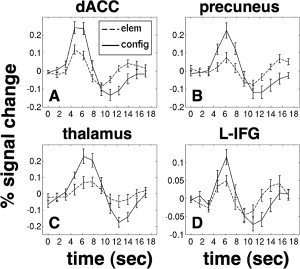
Timecourses of regions showing a condition by time interaction. A: Dorsal anterior cingulate cortex, (coords. 0, 11, 40), not activated on the block level due to mutual cancellation of the differences in the early and late transient responses. This is true of all the regions shown in this figure. B: Precuneus, (coords. 0, −62, −44). C: Medial dorsal nucleus of the thalamus, (coords. 0, −16, 14). D: Left inferior frontal gyrus/insula, (coords. −38, 18, 10).

DISCUSSION

This study sought to obtain detailed information about the temporal behavior of the BOLD signal in a complex cognitive task, in order to aid in the interpretation of a paradoxical finding that we had previously obtained: that performance of a task known to require the hippocampus (the configural condition) induces a negative signal change in that structure, in comparison both to a fixation baseline and to a closely matched but nonhippocampal‐dependent control (elemental) condition [Astur and Constable, 2004]. Through the use of a mixed block/event‐related design, we sought to determine whether or not the negative signal changes observed in the hippocampus (as well as in other regions) had the same temporal relationship to the trial structure of the task as did the positive changes that occurred in different regions. One common interpretation of task‐induced deactivation in the default mode network is that cognitive processes that are implemented by these structures exhibit high tonic activity that tends to occur less during the performance of demanding cognitive tasks [Gusnard and Raichle, 2001]. Greicius and Menon [2004] have argued that activity in this network, which includes the hippocampus, is temporally uncoupled from positive activation associated with sensory stimulation, although it does tend to be suppressed during task performance, leading to findings of deactivation in block design studies. However, as the hippocampus is known to be necessary for performance of the configural condition in the transverse patterning task, our previous results suggest that negative signal changes may also index task‐related activity, as opposed to the suppression of extraneous processes. A finding that negative signal changes are also temporally coupled to trial events and to positive signal changes would provide evidence in favor of the latter hypothesis.

In designing this study, we envisioned two possible outcomes, and were fairly agnostic about which one would result. One was that negative signal changes would be uncoupled from trial events, such that they would be apparent in a block‐design analysis comparing the average signal level during performance of the configural condition with signal during the elemental condition, but would not be timelocked to stimulus presentation, making an event‐related analysis relatively insensitive to them (as illustrated in Fig. 1F). Such a finding would suggest that hippocampal deactivation in the transverse patterning task is attributable to the relative suppression of extraneous cognitive processes. The other outcome that we envisioned was that stimulus presentation would induce a timelocked negative transient, of a similar shape to the positive event‐related transients that are commonly observed in fMRI, as illustrated in Figure 1D. Although one could still imagine a scenario in which such a finding is compatible with the hypothesis of suppression of extraneous processes, a negative transient closely timelocked to stimulus presentation and larger in the configural condition would suggest a more specific role for negative signal changes in the cognitive information processing that supports task performance.

The results of this study did not conform neatly to either of the two scenarios that we have just outlined, but rather to a third scenario that we did not envision prior to conducting the experiment. We found that negative and positive signal changes in this task were indeed temporally dissociable, but not in the way we initially hypothesized. All positive signal changes on the block level (that is, increases in the level of the BOLD signal during the configural condition compared to the elemental condition, shown in red in Fig. 2A) were attributable to transient signal changes in the typical time range observed in event‐related fMRI studies. Stimulus presentation induced a hemodynamic response similar in shape to a gamma density function, which peaked at ∼6 s poststimulus, and was larger in the configural condition. In sharp contrast, none of the negative signal changes (blue areas in Fig. 2A) were attributable to item‐related hemodynamic responses in this time range. In a mixed block/event‐related analysis, using standard hemodynamic models for item‐related and state‐related activity, positive and negative signal changes were completely dissociated (Fig. 2C,D), suggesting that negative signal changes may be temporally uncoupled from stimulus presentation, as suggested by the findings of Greicius and Menon [2004].

Further analyses of our data using empirically derived measures of the hemodynamic response revealed that although negative signal changes were temporally dissociated from positive changes, they were not in fact uncoupled from stimulus presentation. Rather, they systematically occurred in a later time range, peaking at 10–11 s poststimulus. There were no regions that exhibited a truly sustained signal shift in the configural condition. The observed late negative transient accounted for block‐level deactivation not only in the hippocampus, but in much of the default mode network as well, including anterior and posterior midline and cingulate cortices. The observation that default mode deactivation is driven by a stimulus‐locked late‐peaking negative transient is, to our knowledge, a novel finding. However, the finding of an increased response amplitude between different subject groups specific to the poststimulus undershoot has been reported before [Gopinath et al., 2004, 2006], while an increased temporal lag of negative BOLD signal changes relative to positive changes has been reported in visual cortex [Chen et al., 2005; Gardner et al., 2005]. Given these findings, we suspect that signal behavior like that reported here may be present in numerous fMRI studies of higher cognitive processes, and may be revealed through the use of appropriate analysis procedures that measure the shape of the hemodynamic response empirically, rather than using predefined models that have been derived from studies of passive sensory stimulation.

The finding that deactivation and nonactivation on the block level both arise from a late negative transient in the hemodynamic response was unexpected, and must be interpreted carefully. The task employed in this study was somewhat complex, as each visual stimulus presentation induced a motor response and immediate auditory feedback. However, motor response and feedback are important components of many cognitive tasks that are commonly analyzed in both block‐design and event‐related forms, so the present results may be relevant to interpretation of findings of deactivation and nonactivation in a variety of popular paradigms. In the current study, it is highly unlikely that the differential responses seen in the later time range are attributable to the motor response and the auditory feedback. These events occurred equally in both conditions, and the average latency of the response was under 1 s, while the average difference in response time between conditions was ∼300 ms. Even if the observed late negative signals were exclusively associated with processing of the feedback signal, the peak latency of ∼10 s poststimulus is much too late to be considered equivalent to the standard positive hemodynamic response, which is generally seen to peak in about 6 s, as in our study.

The observed late hemodynamic transient occurs in the same time range as the poststimulus undershoot, which is a commonly observed aspect of the standard hemodynamic response, generally measured in paradigms of passive visual stimulation. The undershoot is typically much smaller than the primary positive response, and is not generally thought to arise from a true decrease in neuronal activity, but rather from other factors related to the BOLD signal, such as a sustained increase in Cerebral Blood Volume (CBV) [Buxton et al., 1998, 2004; Mandeville et al., 1999], or in Cerebral Metabolic Rate of Oxygen Consumption (CMRO₂) [Davis et al., 1998; Frahm et al., 1996; Kruger et al., 1996; Lu et al., 2004], both of which are delayed consequences of the initial neural activity and have a negative impact on the BOLD signal. The late negative transients observed in our study, however, may represent a qualitatively different phenomenon, as they occur in some regions with no initial positive response, such as the medial prefrontal cortex, and they are as large as or larger than the initial positive response in other areas such as the dorsal anterior cingulate.

The physiological basis of fMRI deactivation is not well understood, but recent studies indicate, at least in the visual system, that negative BOLD responses are directly related to decreases in neuronal activity, possibly brought about by inhibitory inputs from activated regions [Shmuel et al., 2006; Stefanovic et al., 2004]. The relationship between inhibition and BOLD is complex, as inhibitory inputs are also metabolically demanding and may lead to increases in BOLD, although empirical support for that view has been limited (reviewed by Lauritzen and Gold, 2003]. However, if the main effect of a nonlocal inhibitory input is to reduce the amount of recurrent excitation within an area, then deactivation may result, as suggested by a computational modeling study [Tagamets and Horwitz, 2001]. The present finding of an initial positive BOLD response followed by a profound undershoot in some of the same areas, and a purely negative late response in other areas, is consistent with a scenario of widespread neuronal inhibition as a delayed consequence of the cognitive activity induced by the task. Physiological mechanisms underlying task‐induced deactivation, therefore, may be somewhat distinct from those responsible for the positive BOLD response observed in passive stimulation paradigms. For example, one recent EEG‐fMRI study has demonstrated a link between negative BOLD responses in medial prefrontal cortex and EEG theta rhythm [Mizuhara et al., 2004]. Given that theta rhythm in rodents is specifically associated with interactions between medial prefrontal cortex and the hippocampus [Hyman et al., 2005; Siapas et al., 2005], this provides further evidence that negative BOLD responses in these structures, as seen in the present study, may play a key role in memory performance rather than reflecting the suspension of unrelated cognitive processes. Further studies combining information from metabolic‐based measures such as fMRI and PET with electrophysiological data from humans and animals may help to elucidate the nature of negative signal changes in these areas.

Although the late‐peaking negative transient observed in this study accounted for block‐level deactivation in many areas, we also observed several regions in which an early positive and late negative transient were both larger in the configural condition, leading to mutual cancellation of the two phases of the response, and consequently yielding no significant activation differences on the block level. This was a surprising finding that would not have been obvious had our experiment not been implemented as a mixed block/event‐related design and analyzed with empirical measures of the hemodynamic response. Nonetheless, we have reason to believe that this fortuitous finding has important implications for numerous fMRI studies, not only those of mixed design but for conventional block designs as well. It is conceivable that neuronal activity occurring in many tasks could induce a biphasic hemodynamic response similar to those illustrated in Figure 4. Regions exhibiting such behavior may therefore not be detected in a standard block design experiment, due to mutual cancellation of early and late phases of the response. In some tasks, the timing of single “trials” cannot be uniquely determined, such as extended covert generation of words or navigation in a virtual maze. For such tasks, the presence of biphasic hemodynamic responses may be indistinguishable from nonactivation, representing a fundamental limitation of the technique. However, many tasks can be implemented in either a block or an event‐related manner. Many researchers would tend to choose a block design because of its simpler implementation and superior statistical power, in the absence of any cognitive consideration that would demand an event‐related design. However, a biphasic response may strongly dissociate two conditions, but would be invisible to a conventional block design analysis.

Fortunately, the detection of biphasic responses is not difficult, even in most block paradigms. As long as a task proceeds as a series of discrete trials, and it is acceptable to use a randomized ISI of several seconds, then the shape of the hemodynamic response time locked to trial onset can be empirically estimated, and the suitability of any particular HRF model can be evaluated for further analysis. If late‐peaking transients (or other atypical responses) are not apparent in the estimated responses, then a standard HRF model can be used with impunity, affording all of the statistical advantages of a block design. If, on the other hand, unexpected shapes are observed, then appropriate statistical procedures can be chosen to extract the most pertinent information from the study. Furthermore, it is not necessary to use FIR modeling as we have to generate an adequate empirical estimate of the hemodynamic response. An attractive alternative is the use of basis functions, which allow a hemodynamic response of reasonable complexity to be reconstructed from perhaps four or five regression coefficients, as opposed to using a separate regressor for each time point [Hossein‐Zadeh et al., 2003; Woolrich et al., 2004], thus resulting in greater statistical power. We obtained very similar hemodynamic response estimates through the use of a series of five sine basis functions, both in individual subjects and in group averages (data not shown). However, in most cases the regression coefficients of basis functions are not directly interpretable in isolation without integrating them into an estimate of the hemodynamic response, as would be necessary for a second‐level multisubject analysis. Therefore, in practice it matters little which approach is used to estimate the response, as long as adequate statistical power is available to get a good estimate of the response magnitude within subjects. We caution, however, about one very common approach, which is to use a gamma‐function model along with its partial derivatives with respect to time and dispersion as a basis set [Friston et al., 1998; Henson et al., 2002]. In that approach, only the original gamma parameter estimate is submitted to second‐level analysis across subjects. In that case, the multi‐subject result is almost the same as using only a single model function—or exactly the same, if the derivatives are orthogonalized with respect to the primary model. Nonetheless, gamma basis functions can in fact be integrated into a single estimate of response magnitude suitable for submission to multisubject analysis [Calhoun et al., 2004]. Given the possibility of hemodynamic responses that distinguish between conditions but differ greatly in form from the canonical model, we suggest that the use of flexible empirical estimates may be a more sensitive means of detecting brain activity in certain cases, even within the context of a traditional block design study. Therefore, for any study incorporating a series of discretely timed trials grouped into blocks, we strongly recommend the use of a jittered ISI rather than a strictly periodic presentation, so that the hemodynamic response can be empirically measured.

REFERENCES

- Alvarado MC, Rudy JW ( 1995): Rats with damage to the hippocampal‐formation are impaired on the transverse‐patterning problem but not on elemental discriminations. Behav Neurosci 109: 204–211. [DOI] [PubMed] [Google Scholar]
- Alvarado MC, Wright AA, Bachevalier J ( 2002): Object and spatial relational memory in adult rhesus monkeys is impaired by neonatal lesions of the hippocampal formation but not the amygdaloid complex. Hippocampus 12: 421–433. [DOI] [PubMed] [Google Scholar]
- Amaro E Jr, Barker GJ ( 2006): Study design in fMRI: Basic principles. Brain Cogn 60: 220–232. [DOI] [PubMed] [Google Scholar]
- Astur RS, Constable RT ( 2004): Hippocampal dampening during a relational memory task. Behav Neurosci 118: 667–675. [DOI] [PubMed] [Google Scholar]
- Astur RS, Sutherland RJ ( 1998): Relational learning in humans: The transverse patterning problem. Psychobiology 26: 176–182. [Google Scholar]
- Baron J, Li Y ( 2004): Notes on the use of R for psychology experiments and questionnaires. http://www.psych.upenn.edu/~baron/rpsych/rpsych.html
- Boynton GM, Engel SA, Glover GH, Heeger DJ ( 1996): Linear systems analysis of functional magnetic resonance imaging in human V1. J Neurosci 16: 4207–4221. [DOI] [PMC free article] [PubMed] [Google Scholar]
- Bussey TJ, Clea Warburton E, Aggleton JP, Muir JL ( 1998): Fornix lesions can facilitate acquisition of the transverse patterning task: A challenge for “configural” theories of hippocampal function. J Neurosci 18: 1622–1631. [DOI] [PMC free article] [PubMed] [Google Scholar]
- Buxton RB, Wong EC, Frank LR ( 1998): Dynamics of blood flow and oxygenation changes during brain activation: The balloon model. Magn Reson Med 39: 855–864. [DOI] [PubMed] [Google Scholar]
- Buxton RB, Uludag K, Dubowitz DJ, Liu TT ( 2004): Modeling the hemodynamic response to brain activation. Neuroimage 23 ( Suppl 1): S220‐S233. [DOI] [PubMed] [Google Scholar]
- Calhoun VD, Stevens MC, Pearlson GD, Kiehl KA ( 2004): fMRI analysis with the general linear model: Removal of latency‐induced amplitude bias by incorporation of hemodynamic derivative terms. Neuroimage 22: 252–257. [DOI] [PubMed] [Google Scholar]
- Cato MA, Crosson B, Gokcay D, Soltysik D, Wierenga C, Gopinath K, Himes N, Belanger H, Bauer RM, Fischler IS, Gonzalez‐Rothi L, Briggs RW ( 2004): Processing words with emotional connotation: An FMRI study of time course and laterality in rostral frontal and retrosplenial cortices. J Cogn Neurosci 16: 167–177. [DOI] [PubMed] [Google Scholar]
- Chee MW, Venkatraman V, Westphal C, Siong SC ( 2003): Comparison of block and event‐related fMRI designs in evaluating the word‐frequency effect. Hum Brain Mapp 18: 186–193. [DOI] [PMC free article] [PubMed] [Google Scholar]
- Chen CC, Tyler CW, Liu CL, Wang YH ( 2005): Lateral modulation of BOLD activation in unstimulated regions of the human visual cortex. Neuroimage 24: 802–809. [DOI] [PubMed] [Google Scholar]
- Cohen MS ( 1997): Parametric analysis of fMRI data using linear systems methods. Neuroimage 6: 93–103. [DOI] [PubMed] [Google Scholar]
- Cox RW, Jesmanowicz A ( 1999): Real‐time 3D image registration for functional MRI. Magn Reson Med 42: 1014–1018. [DOI] [PubMed] [Google Scholar]
- Dale AM ( 1999): Optimal experimental design for event‐related fMRI. Hum Brain Mapp 8: 109–114. [DOI] [PMC free article] [PubMed] [Google Scholar]
- Daselaar SM, Prince SE, Cabeza R ( 2004): When less means more: Deactivations during encoding that predict subsequent memory. Neuroimage 23: 921–927. [DOI] [PubMed] [Google Scholar]
- Davachi L, Wagner AD ( 2002): Hippocampal contributions to episodic encoding: Insights from relational and item‐based learning. J Neurophysiol 88: 982–990. [DOI] [PubMed] [Google Scholar]
- Davis TL, Kwong KK, Weisskoff RM, Rosen BR ( 1998): Calibrated functional MRI: Mapping the dynamics of oxidative metabolism. Proc Natl Acad Sci USA 95: 1834–1839. [DOI] [PMC free article] [PubMed] [Google Scholar]
- Dusek JA, Eichenbaum H ( 1998): The hippocampus and transverse patterning guided by olfactory cues. Behav Neurosci 112: 762–771. [DOI] [PubMed] [Google Scholar]
- Erickson KI, Colcombe SJ, Wadhwa R, Bherer L, Peterson MS, Scalf PE, Kramer AF ( 2005): Neural correlates of dual‐task performance after minimizing task‐preparation. Neuroimage 28: 967–979. [DOI] [PubMed] [Google Scholar]
- Forman SD, Cohen JD, Fitzgerald M, Eddy WF, Mintun MA, Noll DC ( 1995): Improved assessment of significant activation in functional magnetic resonance imaging (fMRI): Use of a cluster‐size threshold. Magn Reson Med 33: 636–647. [DOI] [PubMed] [Google Scholar]
- Frahm J, Kruger G, Merboldt KD, Kleinschmidt A ( 1996): Dynamic uncoupling and recoupling of perfusion and oxidative metabolism during focal brain activation in man. Magn Reson Med 35: 143–148. [DOI] [PubMed] [Google Scholar]
- Friston KJ, Fletcher P, Josephs O, Holmes A, Rugg MD, Turner R ( 1998): Event‐related fMRI: Characterizing differential responses. Neuroimage 7: 30–40. [DOI] [PubMed] [Google Scholar]
- Gardner JL, Sun P, Waggoner RA, Ueno K, Tanaka K, Cheng K ( 2005): Difference in temporal dynamics of positive and negative BOLD responses. Proceedings International Society for Magnetic Resonance in Medicine. 13th Annual Meeting. p. 25.
- Gopinath K, Moore A, Peck K, Crosson B, Briggs R ( 2004): Evidence of altered BOLD hemodynamic response in patients with ischemic stroke. Proceedings, International Society for Magnetic Resonance in Medicine, 12th Annual Meeting, p. 1080.
- Gopinath K, Wierenga C, Conway T, Crosson B, Briggs R ( 2006): Differential BOLD hemodynamics in young and elderly: Emphasis on post‐stimulus undershoot. Proceedings, International Society for Magnetic Resonance in Medicine, 14th Annual Meeting, p. 2788.
- Greenhouse SW, Geiser S ( 1959): On methods in the analysis of profile data. Psychometrika 25: 95–112. [Google Scholar]
- Greicius MD, Menon V ( 2004): Default‐mode activity during a passive sensory task: Uncoupled from deactivation but impacting activation. J Cogn Neurosci 16: 1484–1492. [DOI] [PubMed] [Google Scholar]
- Gusnard DA, Raichle ME ( 2001): Searching for a baseline: Functional imaging and the resting human brain. Nat Rev Neurosci 2: 685–694. [DOI] [PubMed] [Google Scholar]
- Henson RN, Shallice T, Gorno‐Tempini ML, Dolan RJ ( 2002): Face repetition effects in implicit and explicit memory tests as measured by fMRI. Cereb Cortex 12: 178–186. [DOI] [PubMed] [Google Scholar]
- Hossein‐Zadeh GA, Ardekani BA, Soltanian‐Zadeh H ( 2003): A signal subspace approach for modeling the hemodynamic response function in fMRI. Magn Reson Imaging 21: 835–843. [DOI] [PubMed] [Google Scholar]
- Hyman JM, Zilli EA, Paley AM, Hasselmo ME ( 2005): Medial prefrontal cortex cells show dynamic modulation with the hippocampal theta rhythm dependent on behavior. Hippocampus 15: 739–749. [DOI] [PubMed] [Google Scholar]
- Kruger G, Kleinschmidt A, Frahm J ( 1996): Dynamic MRI sensitized to cerebral blood oxygenation and flow during sustained activation of human visual cortex. Magn Reson Med 35: 797–800. [DOI] [PubMed] [Google Scholar]
- Lauritzen M, Gold L ( 2003): Brain function and neurophysiological correlates of signals used in functional neuroimaging. J Neurosci 23: 3972–3980. [DOI] [PMC free article] [PubMed] [Google Scholar]
- Liu H, Gao J ( 2000): An investigation of the impulse functions for the nonlinear BOLD response in functional MRI. Magn Reson Imaging 18: 931–938. [DOI] [PubMed] [Google Scholar]
- Liu TT, Frank LR, Wong EC, Buxton RB ( 2001): Detection power, estimation efficiency, and predictability in event‐related fMRI. Neuroimage 13: 759–773. [DOI] [PubMed] [Google Scholar]
- Lu H, Golay X, Pekar JJ, Van Zijl PC ( 2004): Sustained poststimulus elevation in cerebral oxygen utilization after vascular recovery. J Cereb Blood Flow Metab 24: 764–770. [DOI] [PubMed] [Google Scholar]
- Mandeville JB, Marota JJ, Ayata C, Zaharchuk G, Moskowitz MA, Rosen BR, Weisskoff RM ( 1999): Evidence of a cerebrovascular postarteriole windkessel with delayed compliance. J Cereb Blood Flow Metab 19: 679–689. [DOI] [PubMed] [Google Scholar]
- McKiernan KA, Kaufman JN, Kucera‐Thompson J, Binder JR ( 2003): A parametric manipulation of factors affecting task‐induced deactivation in functional neuroimaging. J Cogn Neurosci 15: 394–408. [DOI] [PubMed] [Google Scholar]
- Miezin FM, Maccotta L, Ollinger JM, Petersen SE, Buckner RL. ( 2000): Characterizing the hemodynamic response: Effects of presentation rate, sampling procedure, and the possibility of ordering brain activity based on relative timing. Neuroimage 11(6, Part 1): 735–759. [DOI] [PubMed] [Google Scholar]
- Mizuhara H, Wang LQ, Kobayashi K, Yamaguchi Y ( 2004): A long‐range cortical network emerging with theta oscillation in a mental task. Neuroreport 15: 1233–1238. [DOI] [PubMed] [Google Scholar]
- Otten LJ, Henson RN, Rugg MD ( 2002): State‐related and item‐related neural correlates of successful memory encoding. Nat Neurosci 5: 1339–1344. [DOI] [PubMed] [Google Scholar]
- Papademetris X, Jackowski AP, Schultz RT, Staib LH, Duncan JS ( 2004): Integrated intensity and point‐feature non‐rigid registration In: Barillot C, Haynor D, Hellier P, editors. Saint‐Malo, France: Springer; pp 763–770. [Google Scholar]
- Penny W, Holmes AP ( 2004): Random‐Effects Analysis. Human Brain Function. San Diego: Elsevier; pp 843–850. [Google Scholar]
- Poldrack RA, Rodriguez P ( 2004): How do memory systems interact? Evidence from human classification learning. Neurobiol Learn Mem 82: 324–332. [DOI] [PubMed] [Google Scholar]
- Polli FE, Barton JJ, Cain MS, Thakkar KN, Rauch SL, Manoach DS ( 2005): Rostral and dorsal anterior cingulate cortex make dissociable contributions during antisaccade error commission. Proc Natl Acad Sci USA 102: 15700–15705. [DOI] [PMC free article] [PubMed] [Google Scholar]
- Raichle ME, MacLeod AM, Snyder AZ, Powers WJ, Gusnard DA, Shulman GL ( 2001): A default mode of brain function. Proc Natl Acad Sci USA 98: 676–682. [DOI] [PMC free article] [PubMed] [Google Scholar]
- Reed JM, Squire LR ( 1999): Impaired transverse patterning in human amnesia is a special case of impaired memory for two‐choice discrimination tasks. Behav Neurosci 113: 3–9. [DOI] [PubMed] [Google Scholar]
- Rickard TC, Grafman J ( 1998): Losing their configural mind. Amnesic patients fail on transverse patterning. J Cogn Neurosci 10: 509–524. [DOI] [PubMed] [Google Scholar]
- Rugg MD, Otten LJ, Henson RN ( 2002): The neural basis of episodic memory: Evidence from functional neuroimaging. Philos Trans R Soc Lond B Biol Sci 357: 1097–1110. [DOI] [PMC free article] [PubMed] [Google Scholar]
- Shmuel A, Augath M, Oeltermann A, Logothetis NK ( 2006): Negative functional MRI response correlates with decreases in neuronal activity in monkey visual area V1. Nat Neurosci 9: 569–577. [DOI] [PubMed] [Google Scholar]
- Siapas AG, Lubenov EV, Wilson MA ( 2005): Prefrontal phase locking to hippocampal theta oscillations. Neuron 46: 141–151. [DOI] [PubMed] [Google Scholar]
- Soltysik DA, Peck KK, White KD, Crosson B, Briggs RW ( 2004): Comparison of hemodynamic response nonlinearity across primary cortical areas. Neuroimage 22: 1117–1127. [DOI] [PubMed] [Google Scholar]
- Spence KW ( 1952): The nature of response in discrimination learning. Psychol Rev 59: 89–93. [DOI] [PubMed] [Google Scholar]
- Stark CE, Squire LR ( 2001): When zero is not zero: The problem of ambiguous baseline conditions in fMRI. Proc Natl Acad Sci USA 98: 12760–12766. [DOI] [PMC free article] [PubMed] [Google Scholar]
- Stefanovic B, Warnking JM, Pike GB ( 2004): Hemodynamic and metabolic responses to neuronal inhibition. Neuroimage 22: 771–778. [DOI] [PubMed] [Google Scholar]
- Tagamets MA, Horwitz B ( 2001): Interpreting PET and fMRI measures of functional neural activity: The effects of synaptic inhibition on cortical activation in human imaging studies. Brain Res Bull 54: 267–273. [DOI] [PubMed] [Google Scholar]
- Wager TD, Vazquez A, Hernandez L, Noll DC ( 2005): Accounting for nonlinear BOLD effects in fMRI: Parameter estimates and a model for prediction in rapid event‐related studies. Neuroimage 25: 206–218. [DOI] [PubMed] [Google Scholar]
- Woolrich MW, Behrens TE, Smith SM ( 2004): Constrained linear basis sets for HRF modelling using Variational Bayes. Neuroimage 21: 1748–1761. [DOI] [PubMed] [Google Scholar]