AN AUTOMATIC FEATURE BASED MODEL FOR CELL SEGMENTATION FROM CONFOCAL MICROSCOPY VOLUMES

Abstract

We present a model for the automated segmentation of cells from confocal microscopy volumes of biological samples. The segmentation task for these images is exceptionally challenging due to weak boundaries and varying intensity during the imaging process. To tackle this, a two step pruning process based on the Fast Marching Method is first applied to obtain an over-segmented image. This is followed by a merging step based on an effective feature representation. The algorithm is applied on two different datasets: one from the ascidian Ciona and the other from the plant Arabidopsis. The presented 3D segmentation algorithm shows promising results on these datasets.

1. INTRODUCTION

We consider the problem of segmenting 3D confocal microscopy cell images. The images of samples labeled for cell periphery pose many challenges for traditional image segmentation methods. For instance, the intensity of the cell boundaries in the images has a wide dynamic range. Furthermore, the imaging resolution along the z axis is lower than the resolution in the x-y plane, and thus, the thickness of cell boundaries varies in different planes. Moreover, the presence of other organelles (e.g, the nuclei of the cells) may cause false edges to be present in the cell boundary images. Our preliminary experiments with state-of-the-art segmentation methods, as described below, confirm the difficulty of this type of dataset. To address this problem, we propose an effective algorithm based on the Fast Marching Method (FMM) [1, 2]. The proposed solution first obtains an over-segmented volume with an automatic initialization. The resulting volume is then corrected based on a trained model. We present results on two diverse datasets to demonstrate the effectiveness of the proposed approach.

Examples of membrane (Ciona) or cell wall (Arabidopsis) tagged images can be seen in Fig. 5(a), 7(a), and 7(c). To highlight some typical problems of the existing level-set based methods, we consider two variants of the well known Chan-Vese algorithm (CV) [3]. The first variant is a single level-set function that is initialized with a sphere inside every cell. Fig. 1(a) shows that this method separates the regions with similar characteristics. Therefore, the boundaries of all the cells are extracted as one object, and the joined interiors are recognized as a second object. To obtain an individual segmentation of the cells, another variant of the CV-algorithm [4] is considered. For this variant, a separate level-set function is initialized inside each cell in the image, making the total number of level-set functions equal to the number of the cells. However, because the interiors of the cells have similar characteristics, the level-set functions leak into neighboring cells and produce undesired results. Therefore, Chan-Vese methods are not suitable for membrane images, because they rely on region characteristics, while these images consist mostly of edges. Fig. 1(b) shows an example of the multiple level-sets approach, applied to a cell wall tagged image.

Fig. 5.

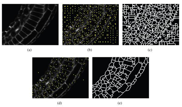
Two-step pruning method based on FMM. (a) An example of a cell boundary image slice, (b) dense seed initialization, (c) highly over segmented image, (d) reduced number of seed points, and (e) reduced over segmentation.

Fig. 7.

(a) Slice of 3D Ciona volume, and (b) the corresponding slice in the 3D segmentation result; (c) Slice of 3D Arabidopsis volume, and (d) the corresponding slice in the 3D segmentation result. Every region is represented by a different color. The segmentation is performed in 3D.

Fig. 1.

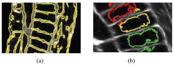
The performance of two different variants of the CV algorithm: (a) single level set (b) multiple level set, where each color represents one level set.

More recently, a modified version of the subjective surface method [5] was shown to be successful in segmenting cell boundary images. The subjective surface method minimizes the volume of a 3D manifold embedded in a 4-D Riemannian space with a metric that is constructed from the image. Fig. 2 shows the result of this algorithm for two different initializations¹. The segmentation contour misses the true boundary in the first example, and attaches to the false boundary in the second case. Again, this can be attributed to the characteristics of membrane tagged images in general.

Fig. 2.

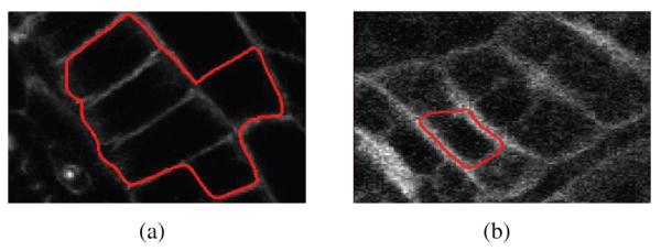
The performance of the subjective surface method with two different initializations.

In summary, the state-of-the-art contour based approaches are highly sensitive to the initialization and do not scale well for 3D confocal images. Another approach to image segmentation consists of the correction of an over-segmented image, as discussed in [6, 7]. The method in [7] minimizes the cost of merging segments across the image, in a linear program formulation. However this method works on consecutive 2D slices instead of approaching the segmentation problem in 3D. The method in [6] uses a trained classifier for the decision whether to merge segments or not, however this method is tailored to images which have nuclei tagging.

In this paper, we propose an efficient yet effective solution for the segmentation of cell boundary images, based on the correction of over-segmentation. The proposed method requires little or no manual interaction in terms of initialization. One of the main advantages of this method is that, due to the automated initialization, there is no need for imaging cell nuclei along with cell membranes. The model requires a training stage for every type of data. This one-time training stage is considerably less work than the manual initialization of every volume. The preliminary results of our experiments are very encouraging in the cell segmentation of confocal microscopy volumes.

The rest of this paper is organized as follows: In Section 2, we explain the FMM based method for obtaining a reasonable over segmentation of a 3D volume, which starts from automatic seed initialization. Section 2.2 describes the feature based merging of the over segmented region, for obtaining the final segmentation of the 3D volume. Section 3 presents the experimental results of this paper. We conclude in Section 4.

2. PROPOSED METHOD

The block diagram of the proposed method is shown in Fig. 3. Our method consists of the following stages: (1) The volume is densely initialized with seed points. These seed points are pruned using a two-step process based on the Fast Marching Method (FMM). This stage automatically reduces the number of seed points, with no human input or any additional nuclei information, and results in an over-segmented volume. (2) The over-segmentation is corrected based on features that capture both edge and region information. The main objective of this stage is to decide whether two neighboring segments of the over-segmented volume belong to the same cell or not. A 3D example of a corrected cell can be seen in Fig. 4. Below, we provide the details of these two stages.

Fig. 3.

Block diagram of the proposed method

Fig. 4.

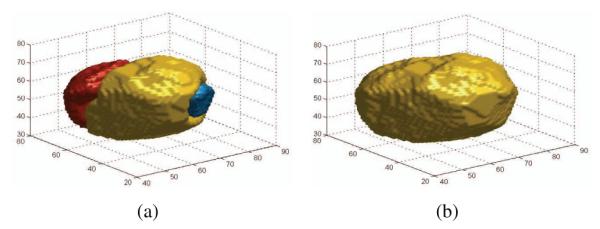
(a) An example of an over-segmented cell, and (b) the corrected segmentation.

2.1. A two-step pruning process based on FMM

The Fast Marching Method (FMM) is generally used to effectively compute geodesic distances in the discrete image domain, by solving an eikonal equation:

$$\mid \nabla T(x,y,z)\mid =F(x,y,z),$$ (1)

where the 6-neighbors of a voxel (3D pixel) are used to estimate the actual distances. Here, F (x, y, z) encodes the relation between neighboring voxels. Thus, the solution T (x, y, z) is simply the Euclidean distance, if F (x, y, z) is constant over the domain. Similarly, if F (x, y, z) is an edge-strength function, then T (x, y, z) provides the geodesic distances based on image gradients.

In the following, we explain the two-step iterative pruning process, and we use a two dimensional implementation of the algorithm for demonstration purposes, as shown in Fig. 5. Note that the algorithm is designed to run over 3D volumes and is evaluated over these volumes in Section 3. The dense initialization with seeds is performed by splitting the given 3D volume into small non-overlapping cubes. The size of the cube is determined by the size of the smallest possible cell in the volume. A seed is then selected within each cube at the minimum intensity voxel location. The dense initialization of the sample image in Fig. 5(a) is shown in Fig. 5(b). Next, FMM is run on the whole volume with these seed points. The result of running FMM with the dense initialization is a highly over segmented image, as shown in Fig. 5(c). To improve upon this, we cluster the initial seed points that are below a selected threshold of the piecewise linear function T (x, y, z), returned by the FMM. This is equivalent to re-assigning one seed point to every valley of T (x, y, z). The reduced number of seed points after the pruning process is shown in the two dimensional example of Fig. 5(d). Finally, a second pass of the fast marching algorithm is run on the volume with the reduced number of seed points. This results in a much less over segmented image, as shown in Fig. 5(e). The pruning process greatly reduces the number of seed points, and thus the total number of segments².

The Fast Marching Method (FMM) is computationally expensive when processing large 3D volumes. Thus, in a practical setting, the volume can be partitioned into smaller overlapping cuboids. The overlapping region should be large enough to include at least one seed point in each of the x, y and z directions. This way, a smooth and consistent output can be derived for the entire volume from the output of running FMM on the partitions.

2.2. Correction of the Over-Segmentations

To correct the over-segmented output of the first stage, we adopt a method that examines the features of the neighboring segments. We use a classifier to make the decision of wether or not to merge two neighboring segments (called pairs). The classifier is trained with examples of the pairs of segments that belong to the same cell (decision = merge), and pairs with a real separating cell boundary (decision = not merge). The two classes are represented in a two dimensional feature space as described below.

2.2.1. Features

Two different features are used to capture both region and boundary properties of neighboring segments. Let S_i and S_j be two arbitrary neighboring segments and B_ij be the corresponding boundary interface.

We compute the difference between the average intensity of the boundary interface and the minimum of the average intensity values inside each of the two segments. This can be written as:

$$f_1={\stackrel{‒}{\mathcal{B}}}_{ij}-\min ({\stackrel{‒}{\mathcal{S}}}_i,{\stackrel{‒}{\mathcal{S}}}_j)$$ (2)

where f₁ and $\left(\stackrel{‒}{.}\right)$ denote the first feature, and the average of the corresponding population, respectively. It is inferred from the above equation that f₁ uses the relative information to discriminate between good and bad boundary candidates. This is meaningful because the membrane intensity covers a wide dynamic range. Note that this feature ensures that cell pairs for which one cell has a brighter interior than the other remain separate. This happens for cells such as the peripheral cells in Fig. 7(a), where the membrane staining is stronger than the rest of the image.

The second feature uses an information theoretic measure:

$$f_2=H\left({\mathcal{B}}_{ij}\right)-H\left(\{{\mathcal{S}}_i,{\mathcal{S}}_j,{\mathcal{B}}_{ij}\}\right),$$ (3)

where H(.) denotes the entropy of the corresponding quantity. This measures the change in entropy between the boundary region and the two segments as a whole. Intuitively, for the false boundaries, the distribution of intensities is more uniform than for real boundaries. Thus, f₂ is expected to be negative if the boundary interface B_ij is a true one, or stay close to zero otherwise.

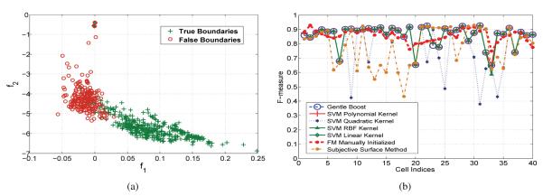
Therefore, a two dimensional feature vector F_ij = [f₁, f₂], is computed for each of the extracted edges after the over-segmentation step. The two dimensional feature space of a sample training set is illustrated in Fig. 6(a).

Fig. 6.

(a) Training examples in the feature space; (b) Comparison of the proposed method using different classifiers, with the manually initialized FMM, and the subjective surface based method from [5] (for 40 Ciona cells).

3. EXPERIMENTAL RESULTS

To show the effectiveness and robustness of the presented approach, we performed our experiments with two different datasets, one from Ascidian Ciona³ and the other form the plant Arabidopsis⁴. First, we aply the two step fast marching method on the raw volumes to obtain the over-segmentation. Then, the possible boundary interfaces B_ij are extracted for the volume and their two dimensional features are computed. These features are then fed to the classifier to obtain the final result. A 3D example of a cell before and after the classifier are shown in Fig. 4(a) and Fig. 4(b), respectively.

We evaluate the performance of our method on forty cells of the Ciona dataset. The comparison metric is the F-measure, which is a volume based error metric and is defined as:

$$F=\frac{2\mathcal{P}\mathcal{R}}{\mathcal{P}+\mathcal{R}}$$ (4)

where P and R are the precision and the recall for a given groundtruth volume.

The presented method is tested using five different classifiers. These classifiers are trained with 300 examples of true boundaries, and 150 examples of false boundaries. The average performance of the method employing different classifiers is shown in Table 1. These results are compared with the F-measure scored by the FMM when manually initialized inside each of these cells, and with the method described in [5]. The best performing classifier, SVM with Linear Kernel, obtains an average F-measure similar to that of the manual initialization, while the other classifiers come close to this value. Also, all the classifiers performed better than the method from [5]. This shows that the feature space specified above, separates the two classes sufficiently to obtain consistent results with various classifiers. Fig. 6(b) illustrates the F-measure of the cells in this experiment for different classifiers. It can be inferred from this figure that the F-measure is lower for certain cells because these cells remained partially over-segmented.

Table 1.

Accuracy of the proposed method using various classifiers. Note that the automatic methods perform as well as the manual initialized FMM and better than the method in [5]

Variations of proposed method	Average F-measure
Gentle-Boost	0.8588
SVM-Linear kernel	0.8625
SVM-Quadratic kernel	0.7853
SVM-Polynomial kernel	0.8598
SVM-RBF kernel	0.8582
Other methods	Average F-measure
Manually Initialized FMM	0.8558
Method from [5]	0.7787

To better observe the effectiveness of our method, we present two illustrative slices of the Ciona and the Arabidopsis datasets in Fig. 7. The segmentation method is run over the 3D images and a slice of the volume is displayed in this figure. Fig. 7(b) shows the corresponding segmentation of the slice of the Ciona in Fig. 7(a). We note that, the small peripheral epidermal cells are particularly challenging. However, the presented method accurately segments many of these cells. The large cells were also correctly segmented, with a few exceptions.

Finally, Fig. 7(c) illustrates a slice of the segmentation of the Arabidopsis, whose corresponding slice in the original volume is shown in Fig. 7(d). This image poses additional difficulty, because the cell walls are very thick. Furthermore, intensity varies within the same cell and there are cell wall portions with many discontinuities. As can be seen in Fig. 7(d), the proposed method performs reasonably well over this dataset. However, sometimes the thick boundaries are mistaken for uniform regions.

4. CONCLUSION

In this work, we develop a general purpose segmentation algorithm which is applicable to 3D confocal microscopy membrane images. The proposed approach first generates an over-segmented version of the desired output, using a two-step pruning process based on the fast marching method. The over-segmentation is then corrected by a merging step using a learned model. In this regard, we propose a two-feature representation that is effective for membrane images. We confirmed the high performance of the presented method through experiments on the Ciona and the Arabidopsis datasets. We showed that the presented method works as well as the manually initialized method, and is potentially generalizable to other 3D images of membrane staining. Future work includes the study of additional features as well as including the thickness of the boundary as a parameter.