

Abstract
Because autosomal genes in sexually reproducing organisms spend on average half their time in each sex, and because the traits that they influence encounter different selection pressures in males and females, the evolutionary responses of one sex are constrained by processes occurring in the other sex. Although intralocus sexual conflict can restrict sexes from reaching their phenotypic optima, no direct evidence currently supports its operation in humans. Here, we show that the pattern of multivariate selection acting on human height, weight, blood pressure and glucose, total cholesterol, and age at first birth differs significantly between males and females, and that the angles between male and female linear (77.8 ± 20.5°) and nonlinear (99.1 ± 25.9°) selection gradients were closer to orthogonal than zero, confirming the presence of sexually antagonistic selection. We also found evidence for intralocus sexual conflict demonstrated by significant changes in the predicted male and female responses to selection of individual traits when cross-sex genetic covariances were included and a significant reduction in the angle between male- and female-predicted responses when cross-sex covariances were included (16.9 ± 15.7°), compared with when they were excluded (87.9 ± 31.6°). We conclude that intralocus sexual conflict constrains the joint evolutionary responses of the two sexes in a contemporary human population.
Keywords: sexually antagonistic selection, intralocus sexual conflict, evolutionary response, humans
1. Introduction
Genetic mechanisms constrain responses to natural selection in all organisms [1–3]. Further constraints on evolutionary responses occur in sexual species with differentiated genders, where most genes are expressed in both females and males. For example, the same traits can encounter different selection pressures in the two sexes (sexually antagonistic selection [4,5]) and the genetic correlations of the traits between the sexes will determine whether they are constrained from reaching their sex-specific optima (intralocus sexual conflict [6]; also called intersexual ontogenetic conflict [7]).
Intralocus sexual conflict is likely to impact a wide range of evolutionary processes [6,8], and its operation has been observed in plants and animals [4,6,9,10] by demonstrating either sexually antagonistic trait selection [11,12] or a negative genetic correlation for fitness between males and females [13–16]. Because the shared traits that mediate these conflicts were not identified in most such studies (for an exception, see [17]; for review, see [6]), they may have underestimated the complexity of intralocus sexual conflict, for selection rarely acts on single traits alone, and most morphological, physiological and life-history traits share genetic correlations [18]. In modern humans, there has been recent interest in testing for intralocus sexual conflict [19,20]. However, there has not yet been any direct evidence for genetic constraints on shared traits because existing longitudinal data on both sexes that include both pedigrees and life-time reproductive success (LRS) have not yet been used to compare selection gradients, cross-sex covariances and predicted responses. Here, we show how these effects interact to constrain the joint responses to selection of human males and females in a contemporary population.
Studying how natural selection acts on traits in contemporary populations became more interesting when methods were developed to analyse the intensities of selection on multiple interacting traits [18,21] and to estimate genetic parameters with maximum-likelihood methods on large sets of complex pedigrees [22]. Initially applied to natural populations of plants and animals [23], these methods demonstrated that responses to natural selection are pervasive and ongoing. Applied more recently to contemporary human populations [24–26], they showed that humans continue to evolve.
Sex-specific selection interacts with genetic constraints shared between the sexes to generate the joint response to selection in males and females. If the responses in one sex are constrained by processes occurring in the other sex, then the phenotype is not optimized for performance in each sex; instead, it has compromises forced upon it by the fact that genes regularly pass through both male and female bodies. Understanding these compromises can help one to explain human sexual dimorphism in morphological, life-history and medically relevant traits, as well as some of the evolutionary puzzles of sexuality [20,27,28]. In this study we asked whether the males and females enrolled in the Framingham Heart Study experience different selection pressures, and, if they do, whether those differences in gender-specific selection combine with cross-sex genetic covariances to constrain responses to selection in both sexes.
2. Material and methods
We estimated the additive genetic variances within and co-variances within and between the sexes, and the selection intensities acting on seven focal traits—height, weight, systolic and diastolic blood pressure, blood glucose, total cholesterol and age at first birth—in 2655 males and 2226 females in the Framingham Heart Study [29], in which three generations totalling 15 877 people nested in 1538 pedigrees have been regularly examined for multiple traits, starting in 1948 and continuing to the present. We used sub-samples in which the necessary information was available.
(a). Study population
The ongoing Framingham Heart Study initially enrolled 5209 men and women (termed the original cohort) from the town of Framingham, MA in 1948. Trained physicians examined these participants every 2 years for a total of 28 times. Original cohort members are predominantly of European ancestry (20% UK, 40% Ireland, 10% Italy, 10% Quebec). An offspring cohort was included in 1971, consisting of 5124 offspring of the original cohort; they have been measured eight times (roughly every 4 years). A third generation cohort has been followed since 2002 but was not included in our analysis because many have not completed reproduction. We obtained human subjects approval from the Yale Institutional Review Board and from the National Institutes of Health dbGaP database. Data were de-identified by the Framingham Heart Study.
(b). Data used
The collective pedigree consists of 15 877 individuals nested within 1538 pedigrees (pedigree size ranged from 2 to 526 individuals with a mean of 8.4) and includes immediate and extended family links. To give an example of how thoroughly traits were measured, 14 173 individuals were measured on average 7.3 times (maximum 28 times) for systolic blood pressure, yielding 104 682 measurements of this trait. Of these individuals, 2383 and 5143 also had one or both parents measured for systolic blood pressure, respectively. We analysed the traits measured across most examinations in the original and offspring cohorts but report here only on the seven that were truly quantitative and allowed us to retain a significant sample size throughout: height, weight, total cholesterol, blood glucose, systolic blood pressure, diastolic blood pressure and age at first birth. Additional details of study design and selection intensities for the other traits—heart disease functional class, average of five heart disease indicators, average of eight indicators of neurological disease, urinalysis albumin, urinalysis glucose, diabetes diagnosis and, for women, age at menopause—are provided in the electronic supplementary material.
We used measurements of traits between the ages of 20 and 60 years, the main reproductive years in humans. We accounted for nonlinear changes in traits (owing to age and year measured) by taking residuals from the surface of a generalized additive model (LOESS; see the electronic supplementary material, figure S1), converting these to the original metric by adding the global mean, and averaging repeated measures to produce a single measure per person [24]. The surface can be estimated accurately from the large number of measures. Traits deviating from normality were log-transformed. Age at first birth was estimated from pedigree and age data. The covariation between traits and LRS was not confounded by reverse causation; that is, the number of children an individual produced did not lead to developmental changes in their observed traits. For example, female weight was not affected by the number of children given birth to previously [24].
(c). Decisions made in the analysis
To represent environmental effects, we included covariates in the multivariate selection analyses: self-reported smoking status, presence/absence of diabetes mellitus, self-reported oestrogen use and self-reported medications for cholesterol and hypertension between ages 20 and 60 years, education and country of origin. Very few women took cholesterol-lowering medication; they were removed from the analysis. Data on country of origin were only collected for the original cohort; we assumed that individuals in the offspring cohort were born in the US. Education was number of years of completed education; those with missing values were assumed to have 8 years. Smoking status indicated whether a person had been recorded as a smoker. LRS was obtained from questionnaires and inferred from pedigrees. We previously demonstrated that the proportion not surviving to age 20 years is so low in modern populations that expanding the measure of fitness to include the effects of mortality before age 20 years would probably have little to no effect on our findings [24].
We controlled for temporal fluctuations (baby boom–bust effects) in LRS and age at first birth (see the electronic supplementary material, figure S2) by separating the population into six groups of differing average fertility by year of birth (birth years 1892–1918, 1919–1925, 1926–1936, 1937–1941, 1942–1946, 1947–1956) and calculated relative fertility by dividing individual measures by the mean for birth groups. Male and female data were adjusted separately. The 5372 women and 4719 men in the original and offspring cohorts were reduced to 2226 and 2655 in the sample analysed for several reasons. We excluded individuals measured fewer than three times for any of the continuous traits. The male sample was reduced due to missing values for age at the latest exam, missing from the pedigree file, age younger than 60 years by the latest examination, or prostate surgery or vasectomy before age 60 years. The female sample was reduced if menopause had not occurred by the latest examination, if values for age at menopause were missing after age 50 years or if reproductive potential ceased unnaturally before age 45 years (hysterectomy, ovaries removed, radiation, chemotherapy, etc.).
(d). Sexual dimorphism of shared traits
We estimated the overall level of sexual dimorphism with a multivariate analysis of variance (MANOVA), entering the seven shared focal traits as dependent variables and sex as the main independent fixed effect. To assess how each shared focal trait differed individually, we used univariate ANOVAs to compare males and females. All seven focal traits were significantly sexually dimorphic (see the electronic supplementary material, table S3), indicating that females are typically shorter and lighter, have higher cholesterol, lower blood pressure and blood glucose, and have their first child at a younger age.
(e). Estimating selection gradients for males and females
We calculated selection gradients (ß) by regressing LRS on phenotypic traits and covariates using multiple linear regression, which included linear, quadratic and cross-product terms for the main phenotypic traits. Regressions were performed separately for males and females. As the sample for age at first birth was considerably smaller owing to individuals with no children, two analyses were performed: with and without age at first birth. Quadratic regression coefficients were doubled as suggested by Stinchcombe et al. [30]. LRS was converted to relative fitness (i.e. modified to a mean of one) and focal traits to zero means and unit variances (as recommended by Lande & Arnold [18]) for both males and females. Using a non-continuous dependent variable (i.e. LRS) in multiple linear regression may violate distributional assumptions and cause problems for estimating significance of ß-values [31]. Therefore, p-values were also obtained using a multiple Poisson regression, where LRS was treated as an integer, and by resampling, where LRS was randomly shuffled in male and female datasets to create null distributions for each ß-value. p-values were derived from the number of times (out of 10 000 simulations) that original ß-values were greater than or equal to the ß pseudo-values. p-values from the Poisson regression and resampling procedure were similar to those from the linear regressions. Mean standardized coefficients [32] were obtained from the multiple linear regression.
(f). Comparing male and female multivariate selection
To test for the presence of sexually antagonistic selection, we compared the strength and direction of selection between males and females using two approaches. First, we used partial F-tests as outlined by Chenoweth & Blows [33], which screen for male–female differences in the magnitude of selection gradients. Second, to check for male–female differences in direction of selection in a multivariate space, we calculated the angle (θ) between vectors of linear selection gradients and also between the dominant vectors of nonlinear selection (eigenvectors, λ) using θ = cos−1(a·b)/∥a∥∥b∥), where  and
and  (described by Lewis et al. [17]). For linear selection gradients, a and b represent the vector of male and female linear selection gradients (ßm, ßf), respectively. For nonlinear selection, a and b represent the dominant vector of γ for males and females (λm, λf), respectively. We also estimated p-values and confidence intervals (CIs) for θ (described below).
(g). Predicted response to selection in males and females
We applied a mixed-effects restricted maximum likelihood (REML) model in ASREML v. 3.0 [22] to pedigrees to estimate the male–female genetic variance–covariance matrix G [34]:
| 2.1 |
G is composed from the within-sex genetic covariance matrices for males (Gm) and females (Gf), and the additive genetic covariance between sexes (B), where BT is the transpose of B. Predicted responses to selection were estimated using a derivative of equation (2.1) of Lande [21], where P−1s was replaced with ß:
| 2.2 |
Δzm and Δzf are predicted vectors of male and female trait changes, estimated using G and the vectors of male–female selection gradients (ßm and ßf), where 1/2 adjusts for equal male and female contributions to offspring. We also examined the potential degree of genetic constraint imposed by B (first test for intralocus sexual conflict at the trait level), by comparing predicted responses obtained from equation (2.2) above (RB=B) to those where this was set to zero (RB=0). p-values for the differences between predicted trait responses (with and without B) were obtained with t-tests that used variances summed from G and ß. We did not predict evolutionary responses to selection past one generation because changes in selection gradients driven by rapid cultural change make projections beyond one generation unreliable. We only projected changes for quantitative traits that were well measured throughout the study.
To examine the potential degree of constraint imposed by the cross-sex covariances (second test for intralocus sexual conflict at the phenotype level, i.e. across all traits jointly), we calculated the angle (θ, formula presented above) between the vectors of male- and female-predicted responses to selection, once when cross-sex covariances were included (RB=B) and once when they were excluded (RB=0). If the angle between male- and female-predicted responses when RB=B is significantly smaller than the angle when RB=0, then cross-sex covariances are constraining male and female responses to selection (i.e. forcing shared traits to evolve more similarly). If these angles are not significantly different, then B is probably not constraining the evolution of shared male and female traits. Testing for a significant difference between these two angles is described below.
In studies where predicted responses to selection have been estimated, it is often difficult to conclude whether they are sufficiently large to be considered significantly different from the mean in the previous generation. Furthermore, when estimating angles (θ) between two vectors, it is important to know whether an angle is close enough to 90° to be scientifically interesting. Therefore, we estimated the significance of such angles by comparing them to simulated null distributions. We randomly shuffled LRS to obtain a null distribution for each selection gradient with no relationship between fitness and traits and randomly shuffled trait values to obtain a null distribution for each genetic variance and covariance with no familial relationships. Pseudo-estimates of selection were used to obtain a null distribution of angles (θ) between male and female linear and male and female nonlinear selection intensities. The pseudo-estimates of selection and genetic covariances (with and without pseudo-estimates of B) were combined in equation (2.2) to obtain a null distribution of trait responses. To test for significant differences between male- and female-predicted responses to selection, and between the angles between male and female linear and male and female nonlinear selection gradients, we noted the number of times in 5000 permutations that the pseudo-estimates were equal to or less than the original estimated response or angle.
Confidence intervals for predicted responses and angles (θ) were estimated using Monte Carlo simulations as described by Byars et al. [24]. The variation in male and female ß, γ and G were randomly sampled 5000 times (ß, γ handled simultaneously) to produce sample distributions for each parameter. Variation in ß and γ were then reflected in the phenotypic covariance matrix among the regression coefficients and in G by the standard errors produced by ASReml. These were then used to generate sample distributions for predicted responses (with and without cross-sex covariances B) and angles (θ), from which 95% CIs were derived. Additionally, we compared the two sample distributions for the angle (θ) between the vectors of male- and female-predicted responses (with and without B) using a Wilcoxon signed-rank test.
3. Results
(a). Patterns of natural selection in males and females
To test the idea that selection on traits in one sex is constrained by selection in the other sex, we first estimated selection intensities on traits in each sex separately using a multiple regression of fitness (completed family size) on each trait, its square, the products of all pairs of traits and the three variables available to control for environmental effects: smoking, country of birth and education level (see the electronic supplementary material, tables S1 and S2). The results (figure 1 and table 1) indicated that directional selection was acting to increase weight, reduce height, decrease total cholesterol and decrease systolic blood pressure more strongly in females than in males, where it was acting more weakly on all of these traits, but in the same direction. Selection was acting to decrease age at first birth more strongly in males than in females. Thus, linear selection intensities on these traits had similar directions but differed in magnitudes between the sexes. Although we did not find any significant linear selection gradients that were directly opposing between the sexes in this analysis, results from further analyses below (θ, partial F-tests), perhaps better suited to detecting sexually antagonistic selection, did uncover significant differences in the magnitude and direction of male–female linear selection gradients.
Figure 1.
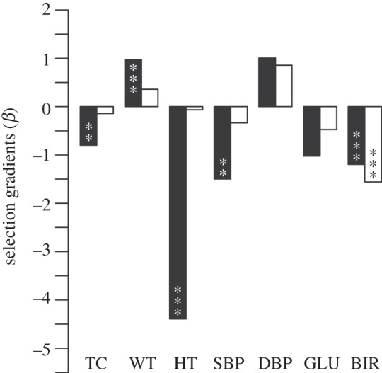
Magnitude and direction of linear selection gradients (β, unstandardized) acting on males (open bars, n = 2655) and females (filled bars, n = 2226) born between 1892 and 1956. Full results are in the electronic supplementary material, tables S1 and S2. TC, total cholesterol; WT, weight; HT, height; SBP/DBP, systolic/diastolic blood pressure; GLU, blood glucose; BIR, age at first birth. p-values are from multiple Poisson regressions (*p < 0.05, **p < 0.01, ***p < 0.001). Overall R2 values were 0.152 and 0.088 for male and female regressions, respectively.
Table 1.
Male and female linear selection gradients (ß) and trait projections (±95% CIs) with (RB) and without (RB=0) cross-sex covariances. mean = trait means; ß ± s.e. = unstandardized selection gradient with s.e.; Pr( > |z|) from a multiple Poisson regression; % var. = percentage of variation in LRS explained; h2 ± s.e. = trait heritability with s.e. Full regression outputs including quadratic and cross-product terms can be found in the electronic supplementary material, tables S1 and S2. TC, total cholesterol; WT, weight; HT, height; SBD/DBP, systolic/diastolic blood pressure; GLU, blood glucose; BIR, age at first birth.
| mean | β ± s.e. | t-value | Pr( > |z|) | % var. | h2 ± s.e. | RB | RB= 0 | |
|---|---|---|---|---|---|---|---|---|
| male | ||||||||
| TC | 220.07 | −0.144 ± 0.207 | −0.694 | 0.557 | 0.008 | 0.62 ± 0.050 | 219.225 ± 0.316 | 220.001 ± 0.158 |
| WT | 80.37 | 0.360 ± 0.269 | 1.34 | 0.224 | 0.169 | 0.48 ± 0.055 | 80.600 ± 0.119 | 80.489 ± 0.053 |
| HT | 173.68 | −0.064 ± 0.953 | −0.067 | 0.95 | 0.037 | 0.84 ± 0.055 | 173.638 ± 0.068 | 173.740 ± 0.041 |
| SBP | 130.44 | −0.335 ± 0.494 | −0.678 | 0.401 | 0.059 | 0.58 ± 0.051 | 130.135 ± 0.134 | 130.486 ± 0.075 |
| DBP | 82.03 | 0.857 ± 0.548 | 1.563 | 0.121 | 0.166 | 0.50 ± 0.053 | 82.015 ± 0.081 | 82.060 ± 0.039 |
| GLU | 93.16 | −0.475 ± 0.355 | −1.34 | 0.701 | 0.006 | 0.27 ± 0.053 | 92.945 ± 0.140 | 93.112 ± 0.063 |
| BIR | 28.91 | −1.559 ± 0.165 | −9.394 | <0.001 | 3.616 | 0.12 ± 0.065 | 28.772 ± 0.115 | 28.833 ± 0.050 |
| female | ||||||||
| TC | 223.87 | −0.799 ± 0.242 | −3.305 | <0.001 | 0.294 | 0.62 ± 0.045 | 223.162 ± 0.294 | 223.309 ± 0.207 |
| WT | 64.72 | 0.972 ± 0.253 | 3.851 | <0.001 | 0.392 | 0.50 ± 0.049 | 64.786 ± 0.113 | 64.706 ± 0.073 |
| HT | 160.24 | −4.393 ± 1.035 | −4.244 | <0.001 | 0.49 | 0.87 ± 0.055 | 160.209 ± 0.062 | 160.172 ± 0.045 |
| SBP | 127.57 | −1.497 ± 0.545 | −2.746 | 0.006 | 0.018 | 0.56 ± 0.046 | 127.399 ± 0.157 | 127.395 ± 0.124 |
| DBP | 78.50 | 1.006 ± 0.607 | 1.657 | 0.098 | 0.036 | 0.53 ± 0.046 | 78.400 ± 0.082 | 78.328 ± 0.063 |
| GLU | 89.11 | −1.022 ± 0.441 | −2.315 | 0.021 | 0.007 | 0.29 ± 0.045 | 88.941 ± 0.111 | 89.005 ± 0.080 |
| BIR | 26.17 | −1.195 ± 0.174 | −6.853 | <0.001 | 3.932 | 0.18 ± 0.057 | 26.080 ± 0.094 | 26.171 ± 0.040 |
For nonlinear selection, sex-specific differences included significant stabilizing selection (i.e. a negative γ) for male but not female height, and significant correlational selection (interaction terms) between glucose (present in urine) and male height and female blood pressure (see the electronic supplementary material, tables S1 and S2). That there was significant stabilizing selection on male height versus negative directional selection on female height suggests different fitness optima for this shared trait. Smoking and country of birth had no significant effect on LRS, whereas education did in both sexes (see the electronic supplementary material, tables S1 and S2): more highly educated men had more offspring and more highly educated women had fewer offspring, on average.
(b). Differences in male and female multivariate selection
The combined effects of selection on all traits suggested that males and females were being selected in different directions in a multivariate space. The differences in selection orientation experienced by the two sexes are summarized by the angles (θ) between the vectors of linear (ßm versus ßf, 77.8 ± 20.5°, 95% CI, p = 0.014) and nonlinear selection (λm versus λf, 99.1 ± 25.9°, p < 0.001), where 90° represents absolute selection constraint and 0° represents complete lack of constraint [35]. Both angles were closer to being orthogonal than parallel (especially so for nonlinear selection), indicating partial constraint. Moreover, partial F-tests indicated an overall significant difference in linear selection between males and females (F13,4850 = 2.14, p = 0.009) that was mostly due to contrasting male–female selection on total cholesterol (p = 0.029), weight (p = 0.003) and height (p < 0.001). Taken together, θ and partial F-test results suggest significant divergence between male and female selection gradients.
(c). Genetic correlations and degree of genetic constraint
To test the idea that genetic correlations between the sexes constrain responses to selection, we estimated the additive genetic variances and covariances of the traits within and between the sexes (table 2). Estimates were obtained from a total of 1538 linked pedigrees by partitioning phenotypic variance into additive genetic and other components with restricted maximum likelihood [22] in a multivariate mixed-effects model where the phenotype of each individual is modelled as the sum of its additive genetic value and other random and fixed effects. Maternal ID was included as a random effect (significant in 11% of the REML analyses) to help represent shared environmental effects; environmental effects were represented by smoking, education and country of origin (significant in 3% of analyses).
Table 2.
Additive genetic covariance matrix (G) for male and female traits. G consists of four submatrices: the additive genetic covariance matrix for (a) males (Gm) and (d) females (Gf) and the additive genetic covariance between (c) the sexes (B) and (b) its transpose (BT). Subscripts m and f refer to males and females, respectively. Values are log10 (×1000). TC, total cholesterol (mg/100 ml); WT, weight (kg); HT, height (cm); SBP/DBP, systolic/diastolic blood pressure (mmHg); GLU, blood glucose (mg/100 ml); BIR, age at first birth. p-values: bold, p < 0.001; bold italic, p < 0.01; italic, p < 0.05; others, p > 0.05. Bonferroni adjustment was applied to p-values (α = 0.05/105 = 0.00047). Cultural (smoking, education, country of origin) and common environment (maternal ID) effects were accounted for in all estimates.
| TCm | WTm | HTm | SBPm | DBPm | GLUm | BIRm | TCf | WTf | HTf | SBPf | DBPf | GLUf | BIRf | |
|---|---|---|---|---|---|---|---|---|---|---|---|---|---|---|
| (a) | (c) | |||||||||||||
| TCm | 2.64 | 3.63 | ||||||||||||
| WTm | −0.07 | 1.86 | −0.44 | 4.28 | ||||||||||
| HTm | −0.09 | 0.48 | 0.23 | −0.13 | 0.56 | 0.26 | ||||||||
| SBPm | 0.19 | 0.03 | −0.05 | 1.26 | 0.61 | −0.15 | −0.08 | 1.77 | ||||||
| DBPm | 0.18 | 0.55 | 0.03 | 1.28 | 0.90 | 0.26 | 0.23 | −0.06 | 1.23 | 1.61 | ||||
| GLUm | −0.04 | −0.25 | −0.17 | 0.83 | 0.47 | 1.20 | −0.17 | 1.50 | −0.06 | 1.30 | 0.68 | 2.10 | ||
| BIRm | −0.53 | −0.27 | 0.33 | −0.47 | −1.65 | −0.27 | 0.63 | −0.11 | 0.08 | 0.05 | 0.28 | −0.52 | −0.54 | 1.54 |
| (b) | (d) | |||||||||||||
| TCf | 3.63 | 2.43 | ||||||||||||
| WTf | −0.22 | 4.28 | −0.50 | 2.86 | ||||||||||
| HTf | −0.10 | 0.56 | 0.26 | −0.12 | 0.47 | 0.23 | ||||||||
| SBPf | −0.03 | 0.49 | −0.001 | 1.77 | 0.11 | 0.64 | 0.02 | 1.47 | ||||||
| DBPf | −0.03 | 0.49 | 0.03 | 1.32 | 1.61 | 0.17 | 0.84 | 0.03 | 1.82 | 1.02 | ||||
| GLUf | 0.37 | 0.60 | 0.03 | 0.74 | 0.54 | 2.10 | 0.31 | 1.17 | −0.06 | 1.26 | 0.74 | 1.07 | ||
| BIRf | −0.68 | 0.87 | 0.41 | −0.56 | −1.24 | −0.59 | 1.54 | −0.47 | 0.08 | 0.23 | −0.75 | −0.57 | −0.83 | 0.97 |
We distinguish between direct and indirect genetic co-variance between the sexes. Direct genetic covariance between the sexes is the genetic covariance in the same trait expressed in each sex. Indirect genetic covariance between the sexes is the genetic covariance between one trait in one sex and another trait in the other sex. Because there was no direct negative genetic covariance between the sexes for any of the traits (table 2b,c), all of the intersexual conflict was caused by indirect negative genetic covariances and by differences in selection in the two sexes. There was significant indirect negative genetic covariance between female height and total cholesterol in males (p = 0.041).
When the sexes were considered separately within the G matrix (table 2a,d), significant negative genetic covariance was also present between height and total cholesterol in males (p < 0.001) and females (p < 0.001). Moreover, these two traits showed complex significant (p < 0.001 in all cases) genetic associations with several other traits: total cholesterol positively correlated with male and female systolic blood pressure and negatively with female weight; height positively correlated with male and female weight and age at first birth, and negatively with male blood glucose.
To explore in more detail the interaction of sexually antagonistic selection with intertrait sexual conflict in constraining responses to selection at the trait level, we predicted the responses of individual traits to selection with and without cross-sex additive genetic covariances of traits (B). The results (table 1, two rightmost columns; figure 2) indicate that including the cross-sex genetic covariances significantly alters the predicted response of the sexes to selection. Including B significantly altered the direction of predicted responses to selection in one male trait (systolic blood pressure), and the magnitude of predicted responses in two male traits (total cholesterol, age at first birth) and one female trait (age at first birth).
Figure 2.
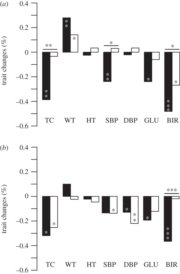
Predicted responses of (a) male and (b) female traits to selection (filled bars, RB; open bars, RB = 0). y-axis represents the percentage change of traits after one generation. Responses were calculated with additive genetic covariances between the sexes (B) included (RB) or set to zero (RB=0). p-values for differences from zero, indicated within the bars, are from comparisons with 5000 random permutations; differences between responses with and without B, indicated above the bars, are from t-tests that used variances summed from G and ß. *p < 0.05, **p < 0.01, ***p < 0.001. TC, total cholesterol; WT, weight; HT, height; SBP/DBP, systolic/diastolic blood pressure; GLU, blood glucose; BIR, age at first birth.
To examine potential genetic constraints at the phenotype level (i.e. across all traits jointly), we also calculated and compared the angles between the vectors of male- and female-predicted responses. They were 16.9 ± 15.7° (95% CI) when cross-sex genetic covariances were included and 87.9 ± 31.6° when they were excluded. These angles were significantly different (p < 0.001, Wilcoxon test), indicating that cross-sex covariances are constraining male and females to respond more similarly for shared traits. This can also be seen visually in figure 2, where all seven shared traits respond in the same direction when RB=B, compared with only three that do so when RB=0.
4. Discussion
(a). The causes of constraint on the joint evolution of the sexes in humans
Contrasting patterns of selection and conflicting genetics both constrain the joint responses to selection of men and women in this population. This result emphasizes how important it is to study the simultaneous evolution of both sexes, which has not previously been tested directly on humans. We were able to do it because of the unusual advantages of the Framingham Heart Study: multiple generations, large samples, reliable measurements and information on pedigrees. The Framingham Heart Study also has disadvantages. It was not designed with our questions in mind, which means we had to work with the traits that were measured, not with those we might have wanted to measure. On the other hand, that the traits studied were selected for medical reasons rather than to investigate sexual selection and conflict suggests that the constraints identified are more general than many—but perhaps not those working on sexual antagonism [6,8]—had previously suspected.
We emphasize that because there was no direct negative genetic covariance between the sexes for any of the traits, all of the intersexual conflict found in this study was caused by indirect negative genetic covariances and by differences in selection in the two sexes.
In the short term, the interaction of sexually antagonistic selection with genetic correlations of traits between the sexes is constraining the evolutionary responses of these contemporary human males and females. In the long term, modifier genes could alter genetic correlations to loosen this constraint [5]. The observed sexual dimorphism for our focal traits suggests that selection acting in the long term has already partially got around these constraints, as has also been demonstrated in model species [36]. Other studies suggest which other human traits may have been under sexually antagonistic selection (e.g. hip width [13,19]).
(b). Contrasting selection and interactions between age at first birth and height
Previous studies examining phenotypic selection gradients for age at first birth have found both potential for the trait to respond genetically and differences between males and females that depended on population and time period. For example, significant linear selection favoured earlier first birth in both sexes in a pre-industrial Finnish population [37], where selection on this trait appeared more intense for women versus men across three populations. More recent evidence from a US population [38] indicated that the magnitude of selection on this trait was similar for males and females. In our sample, selection on first birth appeared slightly more intense for men than women. Demographic and socioeconomical changes have probably influenced how selection has favoured this trait in men and women. Indeed, cultural differences influencing selection acting in men have been reported earlier. For example, Nettle & Pollet [39] found that selection on indicators of male wealth were weaker in industrialized countries and stronger in subsistence societies with extensive polygamy. More generally, it is becoming increasingly apparent that human evolution has been shaped by gene–culture interactions [40].
Patterns of selection acting on male and female heights differed noticeably. Height was the most sexually dimorphic trait (see the electronic supplementary material, table S3) in our study, and it was also one of three traits contributing to the overall significant difference in linear selection between males and females. Moreover, compared with the stabilizing selection on male height, significant linear selection on female height strongly indicated fitness advantages for shorter females. This contrast supports the suggestion by Kanazawa & Novak [41] that the dimorphism in human size emerged not because men got taller but because women became shorter as a response to selection for earlier age at maturity: they traded growth in height for earlier reproduction [26,42]. Correlations between height and age at first birth—both phenotypic and genetic—were significant in females. This suggests that while females may trade height for earlier reproduction as a plastic response on a reaction norm, these traits are also genetically correlated: women who first bear children earlier are genetically predisposed to be shorter on average. And when we included age at first birth in the multiple regression analysis, there was also a significant interaction between female height and first birth (p = 0.009), suggesting that women who reproduce earlier are generally shorter.
In pre-industrial or hunter–gatherer societies, the advantage of being short may have been lost to taller women who had lower rates of infant mortality than did shorter women [39,43,44]. Modern society has greatly reduced infant mortality, causing a transition from mortality-dominated to fertility-dominated reproduction, where selection will now favour earlier reproduction in shorter women [26]. This transition in selection on women may also have directly affected maturation in men; indeed, predicted responses for age at first birth in males and females were significantly greater when the intersexual genetic correlations were included (figure 2).
(c). Negative genetic correlations between height and cholesterol
Female height was indirectly negatively genetically correlated with total cholesterol in males, a negative genetic correlation that was also present when males and females were considered separately (table 2). This suggests that while directional responses in one trait are likely to force opposing directional responses in the other owing to negative pleiotropy, these responses will also be mediated by the significant negative and positive genetic correlations that we found with the other traits. The complexity of these interactions emphasizes the importance of using a multivariate setting to accurately predict trait responses. Our results suggest that of these two traits, only total cholesterol will respond significantly: natural selection is acting to reduce total cholesterol directly in women, and that will also lead to lower cholesterol in men owing to intersexual genetic correlations. This selection pressure to reduce total cholesterol, along with weakening selection pressures beyond the ages of typical reproductive senescence in humans, has probably contributed to differences between the sexes in patterns of cardiovascular disease. Some studies have found that heart disease prevalence in women, which is closely linked with levels of cholesterol, lags behind that in men until post-menopausal age; after that women outpace men [45].
Acknowledgements
We thank the National Evolutionary Synthesis Center (NESCent) for support. D.E. was supported by National Institutes of Health (National Institute on Aging) Grant P30 AG12836. S.C.S. was supported by Yale University and the Wissenschaftskolleg zu Berlin. D.R.G. thanks Charles Lee for facilities and support. S.G.B. was supported by Marie Curie International Fellowship FP7-PEOPLE-2010-IIF-276565, Yale University and Copenhagen University. We thank Craig Walling, Daniel Promislow, and reviewers and editors for helpful comments.
References
- 1.Fisher R. A. 1930. The genetical theory of natural selection. Oxford, UK: The Clarendon Press [Google Scholar]
- 2.Haldane J. B. S. 1932. The causes of evolution. New York, NY: Harper & Brothers [Google Scholar]
- 3.Wright S. 1931. Evolution in Mendelian populations. Genetics 16, 97–159 [DOI] [PMC free article] [PubMed] [Google Scholar]
- 4.Cox R. M., Calsbeek R. 2009. Sexually antagonistic selection, sexual dimorphism, and the resolution of intralocus sexual conflict. Am. Nat. 173, 176–187 10.1086/595841 (doi:10.1086/595841) [DOI] [PubMed] [Google Scholar]
- 5.Rice W. 1984. Sex-chromosomes and the evolution of sexual dimorphism. Evolution 38, 735–742 10.2307/2408385 (doi:10.2307/2408385) [DOI] [PubMed] [Google Scholar]
- 6.Bonduriansky R., Chenoweth S. F. 2009. Intralocus sexual conflict. Trends Ecol. Evol. 24, 280–288 10.1016/j.tree.2008.12.005 (doi:10.1016/j.tree.2008.12.005) [DOI] [PubMed] [Google Scholar]
- 7.Rice W., Chippindale A. 2001. Intersexual ontogenetic conflict. J. Evol. Biol. 14, 685–693 10.1046/j.1420-9101.2001.00319.x (doi:10.1046/j.1420-9101.2001.00319.x) [DOI] [Google Scholar]
- 8.van Doorn G. S. 2009. Intralocus sexual conflict. Ann. NY Acad. Sci. 1168, 52–71 10.1111/j.1749-6632.2009.04573.x (doi:10.1111/j.1749-6632.2009.04573.x) [DOI] [PubMed] [Google Scholar]
- 9.Innocenti P., Morrow E. H. 2010. The sexually antagonistic genes of Drosophila melanogaster. PLoS Biol. 8, e1000335. 10.1371/journal.pbio.1000335 (doi:10.1371/journal.pbio.1000335) [DOI] [PMC free article] [PubMed] [Google Scholar]
- 10.Rice W. R. 1992. Sexually antagonistic genes: experimental evidence. Science 256, 1436–1439 10.1126/science.1604317 (doi:10.1126/science.1604317) [DOI] [PubMed] [Google Scholar]
- 11.Long T. A. F., Rice W. R. 2007. Adult locomotory activity mediates intralocus sexual conflict in a laboratory-adapted population of Drosophila melanogaster. Proc. R. Soc. B 274, 3105–3112 10.1098/rspb.2007.1140 (doi:10.1098/rspb.2007.1140) [DOI] [PMC free article] [PubMed] [Google Scholar]
- 12.Merila J., Sheldon B., Ellegren H. 1998. Quantitative genetics of sexual size dimorphism in the collared flycatcher, Ficedula albicollis. Evolution 52, 870–876 10.2307/2411281 (doi:10.2307/2411281) [DOI] [PubMed] [Google Scholar]
- 13.Chippindale A. K., Gibson J. R., Rice W. R. 2001. Negative genetic correlation for adult fitness between sexes reveals ontogenetic conflict in Drosophila. Proc. Natl Acad. Sci. USA 98, 1671–1675 10.1073/pnas.041378098 (doi:10.1073/pnas.041378098) [DOI] [PMC free article] [PubMed] [Google Scholar]
- 14.Fedorka K. M., Mousseau T. A. 2004. Female mating bias results in conflicting sex-specific offspring fitness. Nature 429, 65–67 10.1038/nature02492 (doi:10.1038/nature02492) [DOI] [PubMed] [Google Scholar]
- 15.Foerster K., Coulson T., Sheldon B. C., Pemberton J. M., Clutton-Brock T. H., Kruuk L. E. B. 2007. Sexually antagonistic genetic variation for fitness in red deer. Nature 447, 1107–1110 10.1038/nature05912 (doi:10.1038/nature05912) [DOI] [PubMed] [Google Scholar]
- 16.Rand D. M., Clark A. G., Kann L. M. 2001. Sexually antagonistic cytonuclear fitness interactions in Drosophila melanogaster. Genetics 159, 173–187 [DOI] [PMC free article] [PubMed] [Google Scholar]
- 17.Lewis Z., Wedell N., Hunt J. 2011. Evidence for strong intralocus sexual conflict in the Indian meal moth, Plodia interpunctella. Evolution 65, 2085–2097 10.1111/j.1558-5646.2011.01267.x (doi:10.1111/j.1558-5646.2011.01267.x) [DOI] [PubMed] [Google Scholar]
- 18.Lande R., Arnold S. 1983. The measurement of selection on correlated characters. Evolution 37, 1210–1226 10.2307/2408842 (doi:10.2307/2408842) [DOI] [PubMed] [Google Scholar]
- 19.Garver-Apgar C. E., Eaton M. A., Tybur J. M., Thompson M. E. 2011. Evidence of intralocus sexual conflict: physically and hormonally masculine individuals have more attractive brothers relative to sisters. Evol. Hum. Behav. 32, 423–432 10.1016/j.evolhumbehav.2011.03.005 (doi:10.1016/j.evolhumbehav.2011.03.005) [DOI] [Google Scholar]
- 20.VanderLaan D. P. D., Forrester D. L. D., Petterson L. J. L., Vasey P. L. P. 2012. Offspring production among the extended relatives of Samoan men and Fa'afafine. PLoS ONE 7, e36088. 10.1371/journal.pone.0036088 (doi:10.1371/journal.pone.0036088) [DOI] [PMC free article] [PubMed] [Google Scholar]
- 21.Lande R. 1980. Sexual dimorphism, sexual selection, and adaptation in polygenic characters. Evolution 34, 292–305 10.2307/2407393 (doi:10.2307/2407393) [DOI] [PubMed] [Google Scholar]
- 22.Gilmour A., Gogel B., Cullis B. 2002. ASReml user guide release 3.0. Hemel Hempstead, UK: VSN International Ltd; See www.vsni.co.uk [Google Scholar]
- 23.Kingsolver J., Hoekstra H. E., Hoekstra J. M., Berrigan D., Vignieri S. N., Hill C. E., Hoang A., Gibert P., Beedi P. 2001. The strength of phenotypic selection in natural populations. Am. Nat. 157, 245–261 10.1086/319193 (doi:10.1086/319193) [DOI] [PubMed] [Google Scholar]
- 24.Byars S. G., Ewbank D., Govindaraju D. R., Stearns S. C. 2010. Colloquium papers: natural selection in a contemporary human population. Proc. Natl Acad. Sci. USA 107(Suppl. 1), 1787–1792 10.1073/pnas.0906199106 (doi:10.1073/pnas.0906199106) [DOI] [PMC free article] [PubMed] [Google Scholar]
- 25.Milot E., Mayer F. M., Nussey D. H., Boisvert M., Pelletier F., Réale D. 2011. Evidence for evolution in response to natural selection in a contemporary human population. Proc. Natl Acad. Sci. USA 108, 17 040–17 045 10.1073/pnas.1104210108 (doi:10.1073/pnas.1104210108) [DOI] [PMC free article] [PubMed] [Google Scholar]
- 26.Stearns S. C., Byars S. G., Govindaraju D. R., Ewbank D. 2010. Measuring selection in contemporary human populations. Nat. Rev. Genet. 11, 611–622 10.1038/nrg2831 (doi:10.1038/nrg2831) [DOI] [PubMed] [Google Scholar]
- 27.Bailey N. W., Zuk M. 2009. Same-sex sexual behavior and evolution. Trends Ecol. Evol. 24, 439–446 10.1016/j.tree.2009.03.014 (doi:10.1016/j.tree.2009.03.014) [DOI] [PubMed] [Google Scholar]
- 28.Ciani A. C., Cermelli P., Zanzotto G. 2008. Sexually antagonistic selection in human male homosexuality. PLoS ONE 3, e2282. 10.1371/journal.pone.0002282 (doi:10.1371/journal.pone.0002282) [DOI] [PMC free article] [PubMed] [Google Scholar]
- 29.Dawber T., Meadors G., Moore F. 1951. Epidemiological approaches to heart disease: the Framingham Study. Am. J. Public Health 41, 279–286 10.2105/AJPH.41.3.279 (doi:10.2105/AJPH.41.3.279) [DOI] [PMC free article] [PubMed] [Google Scholar]
- 30.Stinchcombe J. R., Agrawal A. F., Hohenlohe P. A., Arnold S. J., Blows M. W. 2008. Estimating nonlinear selection gradients using quadratic regression coefficients: double or nothing? Evolution 62, 2435–2440 10.1111/j.1558-5646.2008.00449.x (doi:10.1111/j.1558-5646.2008.00449.x) [DOI] [PubMed] [Google Scholar]
- 31.Mitchell-Olds T. 1987. Regression analysis of natural selection: statistical inference and biological interpretation. Evolution 41, 1149–1161 10.2307/2409084 (doi:10.2307/2409084) [DOI] [PubMed] [Google Scholar]
- 32.Hereford J., Hansen T., Houle D. 2004. Comparing strengths of directional selection: how strong is strong? Evolution 58, 2133–2143 [DOI] [PubMed] [Google Scholar]
- 33.Chenoweth S. F., Blows M. W. 2005. Contrasting mutual sexual selection on homologous signal traits in Drosophila serrata. Am. Nat. 165, 281–289 10.1086/427271 (doi:10.1086/427271) [DOI] [PubMed] [Google Scholar]
- 34.Falconer D. S., Mackay T. F. C. 1996. Introduction to quantitative genetics, 4th edn. Harlow, UK: Prentice-Hall [Google Scholar]
- 35.Blows M. W., Walsh B. 2009. Spherical cows grazing in flatland: constraints to selection and adaptation. In Adaptation and fitness in animal populations (ed. van der Werf), pp. 83–101 Dordrecht, The Netherlands: Springer [Google Scholar]
- 36.Delph L. F., Steven J. C., Anderson I. A., Herlihy C. R., Brodie E. D. 2011. Elimination of a genetic correlation between the sexes via artificial correlational selection. Evolution 65, 2872–2880 10.1111/j.1558-5646.2011.01350.x (doi:10.1111/j.1558-5646.2011.01350.x) [DOI] [PubMed] [Google Scholar]
- 37.Kaar P., Jokela J., Helle T., Kojola I. 1996. Direct and correlative phenotypic selection on life-history traits in three pre-industrial human populations. Proc. R. Soc. Lond. B 263, 1475–1480 10.1098/rspb.1996.0215 (doi:10.1098/rspb.1996.0215) [DOI] [PubMed] [Google Scholar]
- 38.Weeden J., Abrams M., Green M., Sabini J. 2006. Do high-status people really have fewer children? Hum. Nat. 17, 377–392 10.1007/s12110-006-1001-3 (doi:10.1007/s12110-006-1001-3) [DOI] [PubMed] [Google Scholar]
- 39.Nettle D., Pollet T. V. 2008. Natural selection on male wealth in humans. Am. Nat. 172, 658–666 10.1086/591690 (doi:10.1086/591690) [DOI] [PubMed] [Google Scholar]
- 40.Laland K. N., Odling-Smee J., Myles S. 2010. How culture shaped the human genome: bringing genetics and the human sciences together. Nat. Rev. Genet. 11, 137–148 10.1038/nrg2734 (doi:10.1038/nrg2734) [DOI] [PubMed] [Google Scholar]
- 41.Kanazawa S., Novak D. L. 2005. Human sexual dimorphism in size may be triggered by environmental cues. J. Biosoc. Sci. 37, 657–665 10.1017/S0021932004007047 (doi:10.1017/S0021932004007047) [DOI] [PubMed] [Google Scholar]
- 42.Stearns S., Koella J. 1986. The evolution of phenotypic plasticity in life-history traits—predictions of reaction norms for age and size at maturity. Evolution 40, 893–913 10.2307/2408752 (doi:10.2307/2408752) [DOI] [PubMed] [Google Scholar]
- 43.Martorell R., Delgado H., Valverde V., Klein R. 1981. Maternal stature, fertility, and infant mortality. Hum. Biol. 53, 303–312 [PubMed] [Google Scholar]
- 44.Sear R., Allal N., Mace R., Mcgregor I. 2004. Height and reproductive success among Gambian women. Am. J. Hum. Biol. 16, 223 [Google Scholar]
- 45.Choi B. G., McLaughlin M. A. 2007. Why men's hearts break: cardiovascular effects of sex steroids. Endocrinol. Metab. Clin. North Am. 36, 365–377 10.1016/j.ecl.2007.03.011 (doi:10.1016/j.ecl.2007.03.011) [DOI] [PubMed] [Google Scholar]