Simple few-state models reveal hidden complexity in protein folding

Abstract

Markov state models constructed from molecular dynamics simulations have recently shown success at modeling protein folding kinetics. Here we introduce two methods, flux PCCA+ (FPCCA+) and sliding constraint rate estimation (SCRE), that allow accurate rate models from protein folding simulations. We apply these techniques to fourteen massive simulation datasets generated by Anton and Folding@home. Our protocol quantitatively identifies the suitability of describing each system using two-state kinetics and predicts experimentally detectable deviations from two-state behavior. An analysis of the villin headpiece and FiP35 WW domain detects multiple native substates that are consistent with experimental data. Applying the same protocol to GTT, NTL9, and protein G suggests that some beta containing proteins can form long-lived native-like states with small register shifts. Even the simplest protein systems show folding and functional dynamics involving three or more states.

More than fifty years ago, Anfinsen (1) found that primary sequence encodes functional ribonuclease. Today, the process by which proteins self-assemble into their biologically-relevant states remains a key question in biophysics. A modern theory of protein folding must explain a variety of disparate experimental results. First, proteins can fold via a number of mechanisms, ranging from the simplest two-state model (2) to models with more complexity (3). Some proteins may not fold at all—recent work has shown that many eukaryotic proteins are either intrinsically disordered or fold only upon binding to their target (4). The misfolding and aggregation of other proteins have been associated with neurodegenerative disorders such as Alzheimer’s disease (5). A “solution” to the protein folding problem must capture not only the folded and unfolded states but intermediate, disordered, and misfolded states as well.

Kinetic models with two (2) or more (3, 6) states have been the dominant paradigm for understanding protein folding dynamics. This picture generalizes to an arbitrary number of states; the resulting dynamical model is known as the master equation (7). Recently, several labs (8–13) have used molecular dynamics simulations to parameterize discrete time master equations (also known as Markov state models) that describe the folding dynamics of proteins. Such procedures typically involve clustering the observed conformations to determine microstates, then counting transitions between microstates to estimate rates.

Markov state model approaches have typically been limited by two issues. First, the models so constructed have involved hundreds or thousands of states, leading to difficulty making direct connections to experimentally-derived models of folding kinetics. To address this problem, we have developed flux PCCA+ (FPCCA+). Like its precursors PCCA and PCCA+ (14–16), FPCCA+ allows one to construct macrostate models that optimally capture the slow dynamics observed in a microstate model; the advantage of FPCCA+ is in its ability to ignore slow but irrelevant (e.g. low population) dynamics by discarding eigenvectors that have low equilibrium flux. The second difficulty with MSM approaches is that imperfect state decompositions can lead to non-Markovian dynamics, or memory (8, 17, 18), which can bias rate predictions. To address this issue, we have developed a new rate estimation protocol, sliding constraint rate estimation (SCRE), that accurately estimates Markovian rates.

Combining these two approaches allows intuitive few-state models that accurately capture simulated protein folding kinetics in quantitative detail. While several previous studies have demonstrated accurate MSMs, such models have either involved thousands of states (11, 19) or have focused on simple peptide systems (12). The current protocol, however, constructs highly accurate few-state models, enabling quantitative and intuitive connections to experiment. Most importantly, our approach is equally applicable to two-state, three-state, or many-state behavior, with the optimal number of states selected algorithmically.

Applying these methods to 14 folding simulation datasets (20–22) reveals new insights into the nature of two and multi state kinetics. A flux analysis suggests that although model proteins show approximate two-state behavior, additional complexity is apparent. For example, three-state models of the villin headpiece and FiP35 WW domain reveal multiple native states. In contrast, three state models of the beta-containing proteins GTT, NTL9, and protein G (NuG2) show register-shifted native-like states with microsecond lifetimes. Simple but accurate multi-state models can reveal hidden complexity in protein folding.

Results

Relaxation Spectra of Fast-Folding Proteins.

How accurately can two-state models describe simulated protein folding? To answer this question, we analyzed a collection of 14 protein folding datasets (20–22) that were collected using either Anton (23) or Folding@home (24). For each system, a microstate MSM was used to calculate the relaxation timescales and eigenvector fluxes (see Methods). A system with two-state behavior is expected to show a large spectral gap—a single, high-flux timescale that is much slower than the remaining timescales. According to this analysis (Fig. 1), approximate two-state behavior is observed for chignolin, trp-cage (2JOF), HP35 (360 K), FiP35, GTT, NTL9, and A3D. For HP35 (300 K), homeodomain (UVF), BBL, BBA, protein G (NuG2), and lambda, however, two-state models cannot accurately describe the simulated dynamics. For this analysis, we classify a system as two-state if the slowest eigenvector shows a gap in both flux and timescale. More formally, we require that there is no other eigenvector with and 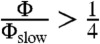, where τ is the relaxation timescale of the eigenvector, τ_slow is the slowest relaxation in the system, Φ is the eigenvector flux, and Φ_slow is the eigenvector flux of the slowest relaxation in the system.

Fig. 1.

For each protein system, the 15 slowest relaxation timescales (also known as implied timescales) of the microstate transition matrix are shown. The equilibrium flux of each corresponding eigenvector is indicated by the darkness of each symbol; fluxes are normalized such that the highest shown flux for each protein is 1. Timescales marked by a circle will be further investigated below using the FPCCA+ and SCRE methods.

FPCCA+/SCRE Produces Accurate Two-State Models.

To validate our analysis protocol, we estimated two-state models for the systems showing approximate two-state behavior. A two-state model is wholly described by two parameters, the fraction folded 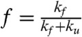and the relaxation timescale τ_r = (k_f + k_u)^-1. We compared our estimates of f and τ_r to previous estimates (21, 22) made using the Hummer reaction coordinate formalism (25) and find quantitative agreement (Fig. 2). Further model validation is provided in Figs. S1–S7.

Fig. 2.

SCRE was used to estimate the fraction folded (A) and relaxation timescale (B) of each protein system. For fraction folded, we estimate error bars by 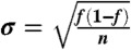, where n is the number of independent folding events in each dataset. For relaxation timescales, we estimate error bars by . The disagreement for GTT is because we analyzed only a single trajectory whereas the previous analysis analyzed two trajectories with distinct folding kinetics.

A key advantage of the FPCCA+/SCRE method, however, is its applicability to systems with multiple states. Indeed, a close examination of the microstate relaxation timescales (Fig. 1) reveals additional high-flux relaxations occurring on timescales somewhat faster than folding. We therefore set out to construct simple models capturing an intermediate level of detail, with the hope that such models might reveal multi-state behavior while still remaining intuitive.

Multi-state Kinetics in BBA Folding Simulations at 325 K.

According to the relaxation spectrum analysis, BBA shows several slow but populated relaxations (Fig. 1); we therefore constructed a 5 state model using FPCCA+/SCRE. The resulting model (Fig. 3) consists of native, near-native, unfolded, and trapped states. The trapped states show non-native beta hairpins and each had microsecond lifetimes and 1% populations. The detected native state shows reasonable agreement with the NMR structure (26) and a population (17%) similar to a previous simulation based model (22%) (22); the near-native state (population 3%) shows a native-like helix but a register shifted beta hairpin.

Fig. 3.

The dominant kinetics of BBA at 325 K. Rate timescales are marked on each edge. The NMR structure (PDB: 1fme) is shown in black. Full rate matrices with error estimates are given in SI Text.

The Villin Headpiece Populates Multiple Native States.

The relaxation spectrum analysis (Fig. 1, red) suggests the presence of two slow, high-flux timescales in a recent simulation of HP35-NLE-NLE at 360 K (22). We therefore used FPCCA+ to construct a three-state model that captures these relaxations. The resulting model consists of unfolded, near-native, and native states (Fig. 4A) with respective populations 77%, 6%, and 18%. The native state shows a strong resemblance to the crystallographic model (PDB: 2f4k Fig. 4(A)), with many conformations showing RMSDs under 2 Å. The near-native state is characterized by partial unraveling of the C terminal helix and shows some similarity to NMR structures (PDB: 1vii, 2ppz) of the wild-type (without norleucine) sequence, which also show partial unraveling of the C terminal helix. The rate matrix relaxation times (400 ns, 70 ns) differ by only a factor of 7, indicating that, at 360 K, HP35 does not show a strong separation of timescales. Given the triangular topology of the rate graph (Fig. 4A), a single reaction coordinate would give a poor description of the system.

Fig. 4.

The dominant kinetics of HP35 (A), FiP35 (B), and GTT (C) are summarized as networks. Simulated structures are shown in rainbow. For HP35 (A), experimental structures are shown in black (crystal structure 2f4k) and gray (NMR structure 1vii). For FiP35 (B), experimental structures are shown in black (holo PDB: 1i8g) and gray (apo PDB: 1i6c). For GTT (C), the experimental holo structure is shown in black. Full rate matrices with error estimates are given in SI Text.

Because the near-native N’ is characterized by an unraveled C terminal helix, we asked whether chemical shifts might be sensitive to the difference between N and N’. To address this question, we used Sparta+ (27) and ShiftX2 (28) to estimate chemical shifts for each state. According to our analysis, amide proton chemical shifts of residues 32 and 33 show differences between the N and N’ states (Fig. 5A and B). Although the differences are small, they are slightly larger than the systematic error inherent in chemical shift prediction. Furthermore, the difference is detected regardless of which chemical shift model is used. We also asked whether the near-native state would show experimentally-observable differences in tertiary structure. To crudely simulate a proton nuclear overhauser experiment, we calculated the r^-6 weighted distance matrix, that is: 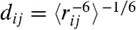. Heat-maps of this quantity suggest that proton NOE experiments could detect subtle differences between the native and near-native states. In particular, the simulated native state shows residues 34 and 35 interacting with residues 29 and 30. In the near-native state, these interactions disappear as the C terminal helix unravels between residue 31 and 35 (Fig. 5D). Temperature melts of NMR observables in the C terminal helix may reveal multiple native substates, although direct observation of N’ may require experimental conditions that perturb the equilibrium between N, N’, and U. Direct kinetic measurements of an N to N’ transition may be difficult due to the fast interconversion rate (precluding relaxation dispersion experiments) and the structural similarity of N and N’.

Fig. 5.

(A, B). Amide proton chemical shifts were calculated for 400 randomly selected conformations from the native and near-native states of HP35. Calculations were performed with both ShiftX2 and Sparta+. The large symbol represents the in-state means of the native and near-native chemical shifts. Error bars correspond to the RMS uncertainty estimated in the parameterization of the ShiftX2 and Sparta+ algorithms; compared to this systematic uncertainty, the statistical uncertainty (SEM) is insignificant. Finally, note that the predictions of ShiftX2 and Sparta+ are not strongly correlated (r² ≈ 0.3), so repeating the calculations with both models gives greater confidence in the results. (C, D). NOE-weighted average distance () is shown for the N (C) and N’ (D) states. Distances are shown for residues 27–35; residues 1–26 show insignificant differences between states N and N’.

How robust is the predicted model to changes in force field and temperature? To address this, we analyzed an independent set (20) of 213 1.2 microsecond simulations. These simulations were held at 300 K and used the amber99sb-ildn (29) force field, which is less helical than the Charmm22* (30) used in the 360 K simulations (31, 32). According to the flux analysis, the 300 K dataset shows considerably less separation of timescales, with several high-flux relaxations occurring in the microsecond range. With many slow relaxations, we do not expect few-state FPCCA+ models to provide an accurate description of the dynamics. Despite the absence of strong three-state behavior, the 300 K simulations indeed sampled near-native conformations similar to those observed in the 360 K data (Fig. 6A). To probe the relative frequency of N versus N’ in the 300 K data, we calculated a 2D histogram of the RMSD to native and near-native conformations (Fig. 6B). The population ratio of N to N’ is approximately 9∶1, roughly consistent with the 360 K data (4∶1). We mention that similar heterogeneity has been observed in previous simulation studies (33, 34).

Fig. 6.

(A). Near-native (gray: 361 K, rainbow: 300 K) conformations are compared for both HP35 datasets. The crystal structure (PDB:2f4k) is shown in black. (B). A 2D RMSD histogram suggests that the 300 K simulations populate both the native and near-native states, with a population ratio of approximately 9∶1. The line x = y was used to separate the N and N’ states.

Apo-Holo Dynamics of the FiP35 WW Domain.

The spectrum of FiP35 (35) at 395 K (21) (Fig. 1, green) suggests the presence of high-flux relaxations on the microsecond and hundred nanosecond timescales. We therefore used FPCCA+ to construct a three-state model for the two dominant relaxations. The three-state model consists of holo (H), apo (A), and unfolded (U) states with respective populations 60%, 2%, and 38%; the observed states show good agreement with NMR structures (holo PDB:1i8g, apo PDB:1i6c) of the related Pin WW domain (36) (Fig. 4B). The estimated rates in this model suggest that reaching the apo state most often occurs via the holo state, as no direct transitions between U and A are observed with the given level of sampling (Fig. 4B). We point out that previous simulation analyses have identified additional near-native dynamics (19), traps (11), and short-lived intermediates (37) in simulations of WW domains.

Slow Register Shift Dynamics: a General Property of Beta Topologies?

The relaxation spectra of the beta-containing protein G (NuG2) (38), NTL9 (39), and GTT (40) (a WW domain) each show a high-flux relaxation (Fig. 1, blue) that occurs on timescales 3–10 times faster than the slowest relaxation. We constructed three-state FPCCA+ models to capture these relaxations. In all three model systems, the observed relaxations correspond to native-like states with register-shifted beta strands; distance maps for GTT are shown in Fig. 7, while PDB structures are shown in Fig. 4C. The populations of the register-shifted states range from 0.1% (GTT) and 0.5% (NTL9) to 1.5% (NuG2); lifetimes of these states range from 0.3 to 3 μs. Finally, our analysis of FiP35 did not detect a similarly populated register shifted state. This may suggest that the populations of register-shifted states are either mutant-specific (GTT vs. FiP35) or dependent on the simulation force field (Charmm22* versus Amber99sb-ildn). A similar register-shifted state is observed in the five state model for BBA (Fig. 3). Register shifted states appear in 4/5 of the beta sheet proteins analyzed here as well as in two recent experimental studies (41, 42). We therefore suggest that slow register-shift dynamics may be a general phenomenon in beta topologies.

Fig. 7.

Distance maps for GTT reveal a register-shifted near-native state. (A). Distance map (C_α) for state N. (B). Distance map for state N’ shows a register shift.

Experimental detection of register shifted states might be possible with isotope labeled 2DIR experiments (43). Alternatively, interconversion between native and near-native states may be detectable by relaxation dispersion NMR, which in principle can detect states with populations under 1.0% (44). Key questions are whether the native and near-native states have distinct chemical shifts and whether the interconversion timescale lies in the millisecond regime. Prediction of chemical shifts for the native and near-native states of NTL9 suggest that certain residues may show experimentally detectable chemical shift differences between the native and near-native states (Fig. S8). In the present high-temperature (≈350 K) simulations, the native and near-native states interconvert on the 1 to 10 μs timescale; at lower temperatures, interconversion times could approach one millisecond.

Discussion

Understanding the Relaxation Spectra of Model Proteins.

Systems with approximate two-state behavior can hide remarkable complexity in their relaxation spectra. Although we have focused on simple model systems, our analysis has shown the presence of remarkably different three state models. At 360 K, HP35 has only a weak separation of timescales, leading to a three-state model where N and N’ interconvert on the hundred nanosecond timescale, only marginally faster than the overall folding reaction. On the other hand, FiP35 shows a cleaner separation of timescales; it reaches its apo state only by first traversing the holo state. The other beta systems (GTT, NTL9, NuG2) show native-like, register-shifted states that might be described as either intermediates or kinetic traps; additional sampling will be required to conclusively decide which.

Comparing HP35 Simulation and Experiment.

We first summarize the experimental consensus on HP35 folding. NMR (45) and x-ray crystallography (46) have revealed the structure of HP35 and its fast-folding (2) mutants. Circular dichroism (47) and other experiments have shown HP35 to be well-folded under ambient temperatures. The double norleucine mutant simulated herein was found (2) to have a melting temperature of 360 K. Finally, IR (48), NMR (49), and fluorescence (2) experiments have shown the folding rate of HP35 to be 3 μs or faster, with the double norleucine mutant showing an 800 ns folding timescale (2, 50).

Despite the success of two-state models in analyzing HP35 experimental results, many experiments demonstrated additional complexity. Laser temperature jump experiments have detected a 100 ns burst-phase (2, 51), believed to be a helix-coil transition within the folded state. A three-state fit (52) of available experimental data leads to an intermediate state that is well-populated (10–50%) in the 300–350 K temperature range. Triplet-triplet energy transfer experiments detected multi-exponential kinetics in contact formation traces (53), leading to a model with native, near-native, intermediate, and unfolded states. In that model, the near-native state was native-like but lacking the same degree of compactness and terminal contact while the intermediate state was characterized by an unfolded C terminal helix and contact between residues 23 and 35.

Our three-state model recapitulates several previous experimental results. Structurally, the native state shows agreement with the crystallographic structure. Temperature jump experiments at 360 K detected equal amplitudes of slow (360 ns) and fast (100 ns) phases; the relaxation timescales are in reasonable agreement with the values predicted by our model (420 ± 100 ns, 70 ± 10 ns). The structural interpretation of the native and near-native states is similar to the model described in (53); in particular, our near-native state shows partial unfolding of the C terminus. Finally, our chemical shift predictions suggest residues 32 and 33 as most able to distinguish the native and near-native states; early NMR work (45) on HP36 and HP45 has shown residues 31 and 32 to have hydrogen exchange protection factors that are intermediate between helix and coil states.

There remain several issues with the current simulation-based model. First, the model overpopulates the unfolded state, as suggested by the experimental (360 K) and simulated (341 K (22)) melting temperatures. Second, the three-state model does not recapitulate the sub-microsecond folding times predicted by temperature jump experiments. The level of disagreement, however, is blurred by the presence of three, not two, states. Exact agreement between simulation and experiment cannot be expected because modern force fields do not fully capture the thermodynamics of the helix-coil transition (32, 54). Finally, TTET experiments at 278 K led to a model with four, not three, states; it is possible that simulations at lower temperature may detect additional states. Finally, we point out that the previous four-state model assumes a linear pathway connecting N, N’, I, and U. Such a pathway has six rate coefficients, exactly as many as our non-linear three-state model.

Conclusion

MSM analysis of 14 massive simulation datasets suggests that two-state models provide a reasonable but approximate description of protein folding dynamics. Simple MSMs constructed using FPCCA+ and SCRE can accurately capture two- and multi-state kinetics with both the number of states and their boundaries computed algorithmically. Applying this approach to HP35 and FiP35 simulations identifies multiple native states consistent with published experimental results. Applying the approach to beta-containing proteins suggests that register shifts can lead to native-like states with long lifetimes. Future improvements in force fields and MSM construction should lead to simulation-based models that are increasingly predictive of experimental results.

Materials and Methods

Benchmark Datasets.

The present analysis focuses on 13 folding datasets (21, 22) collected on the Anton folding machine (23) and one folding dataset (20) collected on Folding@home using Gromacs 4.5 (55). Simulations were performed using either the amber99sb-ildn (29) (HP35-300K, FiP35) or the charmm22* (30) (all other systems) force field. Each trajectory was first subsampled at 50 ns intervals (30 ns for the 300 K HP35 data; 10 ns for the 360 K HP35 data). For the Folding@home dataset, trajectories that were disconnected from all other trajectories (minimum RMSD > 2.0 Å) were discarded prior to clustering; 41 of 254 trajectories were discarded. Anton trajectories were downloaded from DE Shaw Research. For trp-cage, HP35, and FiP35, all atom coordinates were available online. For the remaining systems, only C_α coordinates were available due to bandwidth limitations. We point out that DE Shaw Research has offered to provide all-atom coordinates for other systems via mail; we obtained all-atom coordinates for NTL9 in this manner. For Figs. 3 and 4C, we used the Pulchra software tool (56) to reconstruct all-atom PDB coordinates.

Model Construction.

States are identified using a protocol similar to previous Markov state model approaches (8, 10–13, 57–59). First, the data are clustered into microstates using Ward’s algorithm (60, 61) with the RMSD metric; Ward clustering provides better microstates than previous clustering approaches (Fig. S9). For HP35, FiP35, trp-cage, and NTL9, RMSD calculations were performed using C_α, C_β, C, N, and O atoms. For the other systems, RMSD calculations were performed using C_α coordinates. The number of clusters is chosen such that 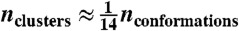; we find that this choice provides a good compromise between clustering accuracy (large n_clusters) and reliable statistics (small n_clusters). For BBA, somewhat more microstates were required. Clustering details (number of states, clusters, data storage frequency, and MSM lagtime) are provided in Table S1. A strongly ergodic, reversible transition matrix (57) is estimated for the microstate model. After clustering, FPCCA+ is used to construct a macrostate model that captures the slowest relevant relaxations in the data.

FPCCA+.

The PCCA+ algorithm constructs a macrostate model that is most consistent with the underlying microstate model (15, 16). It does so by capturing the space spanned by the slowest eigenvectors of the microstate transition matrix. However, one possible problem with PCCA+ is that some slow eigenvectors may correspond to small population changes, which can be quantified by defining the eigenvector flux to be Φ_n = ‖ϕ_n‖², where ϕ_n is the nth π-normalized eigenvector (see SI Text for derivation). To construct macrostates that have significant populations, one can discard any slow eigenvectors that contribute insignificant amounts of equilibrium flux. We call this approach flux PCCA+ (FPCCA+). It is worth mentioning that FPCCA+ is essentially just using PCCA+ to selectively model a user-specified subset of the eigenvectors; the original PCCA+ algorithm involved selecting just the slowest n eigenvectors. For the FPCCA+ models constructed herein, we selected eigenvectors by choosing dual cutoffs for both implied timescale (τ_c) and for flux (Φ_c). We then used FPCCA+ to model all eigenmodes that satisfy both τ > τ_c and Φ > Φ_c. A graphical depiction of these cutoffs is shown in Fig. S2. We point out that FPCCA+ is similar in spirit to “dynamical fingerprint” analysis (62).

Sliding Constraint Rate Estimation (SCRE).

To estimate accurate rate constants that are unbiased by non-Markovian behavior, we have developed the SCRE approach to rate estimation. Given a set of simulations that have been assigned to states , one can calculate a matrix of transition counts from state i to j (C_ij(τ)) that were observed with a lagtime (or sampling window) of τ. The log likelihood of a fixed lagtime transition matrix T(τ) is given by 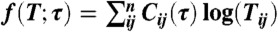(63). To estimate rate matrices, we express the transition matrix in terms of the generating rate matrix T(τ) = exp(Kτ), leading to ; here exp refers to matrix exponential, while log refers to the scalar logarithm. Maximizing the log likelihood with respect to K gives a maximum likelihood estimate of the rate matrix (12). In practice we use detailed balance to fix 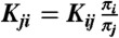, where the equilibrium populations π_i are estimated using a fixed-lagtime reversible transition matrix (57) with minimal lagtime. We also constrain the sparsity structure of K_ij to that observed in the transition matrix; this reduces the number of parameters. Likelihood maximization is performed using the downhill simplex algorithm.

It is important to estimate rates at a lagtime sufficiently long that the rates are Markovian, as otherwise rates will be biased by fast nonproductive fluctuations. On the other hand, too long a lagtime will lead to aliasing of the faster processes and large statistical uncertainties. Furthermore, the Markovian lagtime of one process may be longer than the other timescales in the system; this implies that a single lagtime might not allow accurate modeling all of the observed dynamics. As a solution, we propose the following algorithm to extract each rate constant from its shortest Markovian lagtime. For the first iteration, l is set to 1. Let τ_s denote the time spacing between successive trajectory frames.

1. Calculate the counts C(lτ_s) at lagtime lτ_s.

2. Use C(lτ_s) to estimate K(lτ_s) using likelihood maximization.

3. Check for (Markovian) convergence: if K_ij(lτ_s) = K_ij((l - 1)τ_s), then fix K_ij to be the current values.

4. Increment l by 1 and repeat.

Presently, we estimate convergence graphically by manual inspection, but we are currently developing a fully automated approach. The lagtime for a given rate is chosen such to be the shortest lagtime where the given rate has plateaued. Good state decompositions will give rate elements that level immediately, while poor state decompositions may require long lagtimes to converge. Using this algorithm, each rate K_ij is estimated at its minimal Markovian lagtime. A key advantage of SCRE is that it can, if necessary, estimate each K_ij with a different lagtime. In contrast, previous methods tend to estimate all n² rate elements at a single chosen lagtime. The use of a single lagtime can be problematic in systems where the rates span a large range of timescales; using too short a lagtime will lead to biased kinetics, while using too long a lagtime will alias the faster dynamics observed in the system. We further validate the SCRE method in the SI Text.

Software Availability.

All analysis code (Ward clustering, FPCCA+ , SCRE) is freely available in MSMBuilder 2.5 (https://simtk.org/home/msmbuilder) (9, 57). The tutorial for MSMBuilder 2.5 applies Ward clustering, FPCCA+ , and SCRE to analyze simulations of alanine dipeptide (see SI Text for details).

References

- 1.Anfinsen C, Haber E, Sela M, White F., Jr The kinetics of formation of native ribonuclease during oxidation of the reduced polypeptide chain. Proc Natl Acad Sci USA. 1961;47:1309–1314. doi: 10.1073/pnas.47.9.1309. [DOI] [PMC free article] [PubMed] [Google Scholar]
- 2.Kubelka J, Chiu T, Davies D, Eaton W, Hofrichter J. Sub-microsecond protein folding. J Mol Biol. 2006;359:546–553. doi: 10.1016/j.jmb.2006.03.034. [DOI] [PubMed] [Google Scholar]
- 3.Kim P, Baldwin R. Intermediates in the folding reactions of small proteins. Annu Rev Biochem. 1990;59:631–660. doi: 10.1146/annurev.bi.59.070190.003215. [DOI] [PubMed] [Google Scholar]
- 4.Dyson H, Wright P. Coupling of folding and binding for unstructured proteins. Curr Opin Struct Biol. 2002;12:54–60. doi: 10.1016/s0959-440x(02)00289-0. [DOI] [PubMed] [Google Scholar]
- 5.Hardy J, Selkoe D. The amyloid hypothesis of alzheimer’s disease: progress and problems on the road to therapeutics. Science. 2002;297:353–356. doi: 10.1126/science.1072994. [DOI] [PubMed] [Google Scholar]
- 6.Bai Y, Sosnick T, Mayne L, Englander SW. Protein folding intermediates: native-state hydrogen exchange. Science. 1995;269:192–197. doi: 10.1126/science.7618079. [DOI] [PMC free article] [PubMed] [Google Scholar]
- 7.van Kampen N. Stochastic Processes in Physics and Chemistry. Amsterdam: North Holland; 2007. [Google Scholar]
- 8.Prinz J, et al. Markov models of molecular kinetics: Generation and validation. J Chem Phys. 2011;134:174105–174128. doi: 10.1063/1.3565032. [DOI] [PubMed] [Google Scholar]
- 9.Bowman G, Huang X, Pande V. Using generalized ensemble simulations and markov state models to identify conformational states. Methods. 2009;49:197–201. doi: 10.1016/j.ymeth.2009.04.013. [DOI] [PMC free article] [PubMed] [Google Scholar]
- 10.Chodera J, Singhal N, Pande V, Dill K, Swope W. Automatic discovery of metastable states for the construction of markov models of macromolecular conformational dynamics. J Chem Phys. 2007;126:155101–155118. doi: 10.1063/1.2714538. [DOI] [PubMed] [Google Scholar]
- 11.Noé F, Schütte C, Vanden-Eijnden E, Reich L, Weikl T. Constructing the equilibrium ensemble of folding pathways from short off-equilibrium simulations. Proc Natl Acad Sci U S A. 2009;106:19011–19016. doi: 10.1073/pnas.0905466106. [DOI] [PMC free article] [PubMed] [Google Scholar]
- 12.Buchete N, Hummer G. Coarse master equations for peptide folding dynamics. J Phys Chem B. 2008;112:6057–6069. doi: 10.1021/jp0761665. [DOI] [PubMed] [Google Scholar]
- 13.Buchner GS, Murphy RD, Buchete NV, Kubelka J. Dynamics of protein folding: Probing the kinetic network of folding-unfolding transitions with experiment and theory. Biochem Biophys Acta. 2011;1814:1001–1020. doi: 10.1016/j.bbapap.2010.09.013. [DOI] [PubMed] [Google Scholar]
- 14.Deuflhard P, Huisinga W, Fischer A, Schütte C. Identification of almost invariant aggregates in reversible nearly uncoupled markov chains. Lin Alg Appl. 2000;315:39–59. [Google Scholar]
- 15.Deuflhard P, Weber M. Robust perron cluster analysis in conformation dynamics. Lin Alg Appl. 2005;398:161–184. [Google Scholar]
- 16.Kube S, Weber M. A coarse graining method for the identification of transition rates between molecular conformations. J Chem Phys. 2007;126:24103–24113. doi: 10.1063/1.2404953. [DOI] [PubMed] [Google Scholar]
- 17.Sarich M, Noé F, Schütte C. On the approximation quality of markov state models. Multiscale Model Simul. 2010;8:1154–1177. [Google Scholar]
- 18.Prinz J, Keller B, Noé F. Probing molecular kinetics with markov models: metastable states, transition pathways and spectroscopic observables. Phys Chem Chem Phys. 2011;13:16912–16927. doi: 10.1039/c1cp21258c. [DOI] [PubMed] [Google Scholar]
- 19.Lane T, Bowman G, Beauchamp K, Voelz V, Pande V. Markov state model reveals folding and functional dynamics in ultra-long md trajectories. J Am Chem Soc. 2011;133:18413–18419. doi: 10.1021/ja207470h. [DOI] [PMC free article] [PubMed] [Google Scholar]
- 20.Beauchamp K, Ensign D, Das R, Pande V. Quantitative comparison of villin headpiece subdomain simulations and triplet–triplet energy transfer experiments. Proc Natl Acad Sci U S A. 2011;108:12734–12739. doi: 10.1073/pnas.1010880108. [DOI] [PMC free article] [PubMed] [Google Scholar]
- 21.Shaw DE, et al. Atomic-level characterization of the structural dynamics of proteins. Science. 2010;330:341–346. doi: 10.1126/science.1187409. [DOI] [PubMed] [Google Scholar]
- 22.Lindorff-Larsen K, Piana S, Dror R, Shaw D. How fast-folding proteins fold. Science. 2011;334:517–520. doi: 10.1126/science.1208351. [DOI] [PubMed] [Google Scholar]
- 23.Shaw D, et al. Anton, a special-purpose machine for molecular dynamics simulation. Commun ACM. 2008;51:91–97. [Google Scholar]
- 24.Shirts M, Pande V. Screen savers of the world unite! Science. 2000;290:1903–1904. doi: 10.1126/science.290.5498.1903. [DOI] [PubMed] [Google Scholar]
- 25.Best R, Hummer G. Reaction coordinates and rates from transition paths. Proc. Natl. Acad. Sci USA. 2005;102:6732–6737. doi: 10.1073/pnas.0408098102. [DOI] [PMC free article] [PubMed] [Google Scholar]
- 26.Sarisky C, Mayo S. The beta-beta-alpha fold: explorations in sequence space. J Mol Biol. 2001;307:1411–1418. doi: 10.1006/jmbi.2000.4345. [DOI] [PubMed] [Google Scholar]
- 27.Shen Y, Bax A. Sparta+: a modest improvement in empirical nmr chemical shift prediction by means of an artificial neural network. J Biomol NMR. 2010;48:13–22. doi: 10.1007/s10858-010-9433-9. [DOI] [PMC free article] [PubMed] [Google Scholar]
- 28.Han B, Liu Y, Ginzinger S, Wishart D. Shiftx2: significantly improved protein chemical shift prediction. J Biomol NMR. 2011;50:43–57. doi: 10.1007/s10858-011-9478-4. [DOI] [PMC free article] [PubMed] [Google Scholar]
- 29.Lindorff-Larsen K, et al. Improved side-chain torsion potentials for the amber ff99sb protein force field. Proteins: Struct, Funct, Bioinf. 2010;78:1950–1958. doi: 10.1002/prot.22711. [DOI] [PMC free article] [PubMed] [Google Scholar]
- 30.Piana S, Lindorff-Larsen K, Shaw D. How robust are protein folding simulations with respect to force field parameterization? Biophys J. 2011;100:L47–L49. doi: 10.1016/j.bpj.2011.03.051. [DOI] [PMC free article] [PubMed] [Google Scholar]
- 31.Best R, Buchete N, Hummer G. Are current molecular dynamics force fields too helical? Biophys J. 2008;95:L07–L09. doi: 10.1529/biophysj.108.132696. [DOI] [PMC free article] [PubMed] [Google Scholar]
- 32.Lindorff-Larsen K, et al. Systematic validation of protein force fields against experimental data. PloS one. 2012;7:e32131. doi: 10.1371/journal.pone.0032131. [DOI] [PMC free article] [PubMed] [Google Scholar]
- 33.Freddolino P, Schulten K. Common structural transitions in explicit-solvent simulations of villin headpiece folding. Biophys J. 2009;97:2338–2347. doi: 10.1016/j.bpj.2009.08.012. [DOI] [PMC free article] [PubMed] [Google Scholar]
- 34.Ensign D, Kasson P, Pande V. Heterogeneity even at the speed limit of folding: large-scale molecular dynamics study of a fast-folding variant of the villin headpiece. J Mol Biol. 2007;374:806–816. doi: 10.1016/j.jmb.2007.09.069. [DOI] [PMC free article] [PubMed] [Google Scholar]
- 35.Jager M, et al. Structure-function-folding relationship in a ww domain. Proc Natl Acad Sci U S A. 2006;103:10648–10653. doi: 10.1073/pnas.0600511103. [DOI] [PMC free article] [PubMed] [Google Scholar]
- 36.Wintjens R, et al. 1 h nmr study on the binding of pin1 trp-trp domain with phosphothreonine peptides. J Biol Chem. 2001;276:25150–25156. doi: 10.1074/jbc.M010327200. [DOI] [PubMed] [Google Scholar]
- 37.Krivov S. The free energy landscape analysis of protein (fip35) folding dynamics. J Phys Chem B. 2011;115:12315–12324. doi: 10.1021/jp208585r. [DOI] [PubMed] [Google Scholar]
- 38.Nauli S, Kuhlman B, Baker D. Computer-based redesign of a protein folding pathway. Nat Struct Biol. 2001;8:602–605. doi: 10.1038/89638. [DOI] [PubMed] [Google Scholar]
- 39.Horng J, Moroz V, Raleigh D. Rapid cooperative two-state folding of a miniature alpha-beta protein and design of a thermostable variant. J Mol Biol. 2003;326:1261–1270. doi: 10.1016/s0022-2836(03)00028-7. [DOI] [PubMed] [Google Scholar]
- 40.Piana S, et al. Computational design and experimental testing of the fastest-folding β-sheet protein. J Mol Biol. 2011;405:43–48. doi: 10.1016/j.jmb.2010.10.023. [DOI] [PubMed] [Google Scholar]
- 41.Kührová P, De Simone A, Otyepka M, Best RB. Force-field dependence of chignolin folding and misfolding: Comparison with experiment and redesign. Biophys J. 2012;102:1897–1906. doi: 10.1016/j.bpj.2012.03.024. [DOI] [PMC free article] [PubMed] [Google Scholar]
- 42.Evans MR, Gardner KH. Slow transition between two β-strand registers is dictated by protein unfolding. J Am Chem Soc. 2009;131:11306–11307. doi: 10.1021/ja9048338. [DOI] [PMC free article] [PubMed] [Google Scholar]
- 43.Chung H, Ganim Z, Jones K, Tokmakoff A. Transient 2d ir spectroscopy of ubiquitin unfolding dynamics. Proc Natl Acad Sci USA. 2007;104:14237–14242. doi: 10.1073/pnas.0700959104. [DOI] [PMC free article] [PubMed] [Google Scholar]
- 44.Korzhnev D, Kay L. Probing invisible, low-populated states of protein molecules by relaxation dispersion nmr spectroscopy: an application to protein folding. Acc Chem Res. 2008;41:442–451. doi: 10.1021/ar700189y. [DOI] [PubMed] [Google Scholar]
- 45.McKnight C, Matsudaira P, Kim P. NMR structure of the 35-residue villin headpiece subdomain. Nat Struct Biol. 1997;4:180–184. doi: 10.1038/nsb0397-180. [DOI] [PubMed] [Google Scholar]
- 46.Chiu T, et al. High-resolution x-ray crystal structures of the villin headpiece subdomain, an ultrafast folding protein. Proc Natl Acad Sci USA. 2005;102:7517–7522. doi: 10.1073/pnas.0502495102. [DOI] [PMC free article] [PubMed] [Google Scholar]
- 47.McKnight J, Doering D, Matsudaira P, Kim P. A thermostable 35-residue subdomain within villin headpiece. J Mol Biol. 1996;260:126–134. doi: 10.1006/jmbi.1996.0387. [DOI] [PubMed] [Google Scholar]
- 48.Brewer S, Song B, Daniel P, Dyer R. Residue specific resolution of protein folding dynamics using isotope-edited infrared temperature jump spectroscopy. Biochemistry. 2007;46:3279–3285. doi: 10.1021/bi602372y. [DOI] [PubMed] [Google Scholar]
- 49.Wang M, et al. Dynamic nmr line-shape analysis demonstrates that the villin headpiece subdomain folds on the microsecond time scale. J Am Chem Soc. 2003;125:6032–6033. doi: 10.1021/ja028752b. [DOI] [PubMed] [Google Scholar]
- 50.Cellmer T, Buscaglia M, Henry E, Hofrichter J, Eaton W. Making connections between ultrafast protein folding kinetics and molecular dynamics simulations. Proc Natl Acad Sci U S A. 2011;108:6103–6108. doi: 10.1073/pnas.1019552108. [DOI] [PMC free article] [PubMed] [Google Scholar]
- 51.Kubelka J, Eaton W, Hofrichter J. Experimental tests of villin subdomain folding simulations. J Mol Biol. 2003;329:625–630. doi: 10.1016/s0022-2836(03)00519-9. [DOI] [PubMed] [Google Scholar]
- 52.Kubelka J, Henry E, Cellmer T, Hofrichter J, Eaton W. Chemical, physical, and theoretical kinetics of an ultrafast folding protein. Proc Natl Acad Sci USA. 2008;105:18655–18662. doi: 10.1073/pnas.0808600105. [DOI] [PMC free article] [PubMed] [Google Scholar]
- 53.Reiner A, Henklein P, Kiefhaber T. An unlocking/relocking barrier in conformational fluctuations of villin headpiece subdomain. Proc Natl Acad Sci USA. 2010;107:4955–4960. doi: 10.1073/pnas.0910001107. [DOI] [PMC free article] [PubMed] [Google Scholar]
- 54.Best R, Hummer G. Optimized molecular dynamics force fields applied to the helix- coil transition of polypeptides. J Phys Chem B. 2009;113:9004–9015. doi: 10.1021/jp901540t. [DOI] [PMC free article] [PubMed] [Google Scholar]
- 55.Hess B, Kutzner C, Van Der Spoel D, Lindahl E. Gromacs 4: Algorithms for highly efficient, load-balanced, and scalable molecular simulation. J Chem Theory Comput. 2008;4:435–447. doi: 10.1021/ct700301q. [DOI] [PubMed] [Google Scholar]
- 56.Rotkiewicz P, Skolnick J. Fast procedure for reconstruction of full-atom protein models from reduced representations. J Comput Chem. 2008;29:1460–1465. doi: 10.1002/jcc.20906. [DOI] [PMC free article] [PubMed] [Google Scholar]
- 57.Beauchamp K, et al. Msmbuilder2: Modeling conformational dynamics at the picosecond to millisecond scale. J Chem Theory Comput. 2011;7:3412–3419. doi: 10.1021/ct200463m. [DOI] [PMC free article] [PubMed] [Google Scholar]
- 58.Bowman GR, Beauchamp KA, Boxer G, Pande VS. Progress and challenges in the automated construction of Markov state models for full protein systems. J Chem Phys. 2009;131:124101–124112. doi: 10.1063/1.3216567. [DOI] [PMC free article] [PubMed] [Google Scholar]
- 59.Noé F, Fischer S. Transition networks for modeling the kinetics of conformational change in macromolecules. Curr Opin Struct Biol. 2008;18:154–162. doi: 10.1016/j.sbi.2008.01.008. [DOI] [PubMed] [Google Scholar]
- 60.Ward J., Jr Hierarchical grouping to optimize an objective function. J Am Stat Assoc. 1963;58:236–244. [Google Scholar]
- 61.Mullner D. Modern hierarchical, agglomerative clustering algorithms. 2011. Arxiv.
- 62.Noé F, et al. Dynamical fingerprints for probing individual relaxation processes in biomolecular dynamics with simulations and kinetic experiments. Proc Natl Acad Sci U S A. 2011;108:4822–4827. doi: 10.1073/pnas.1004646108. [DOI] [PMC free article] [PubMed] [Google Scholar]
- 63.Schütte C, Noé F, Lu J, Sarich M, Vanden-Eijnden E. Markov state models based on milestoning. J Chem Phys. 2011;134:204105–204120. doi: 10.1063/1.3590108. [DOI] [PubMed] [Google Scholar]
Associated Data
This section collects any data citations, data availability statements, or supplementary materials included in this article.