Energetic costs of cellular computation

Abstract

Cells often perform computations in order to respond to environmental cues. A simple example is the classic problem, first considered by Berg and Purcell, of determining the concentration of a chemical ligand in the surrounding media. On general theoretical grounds, it is expected that such computations require cells to consume energy. In particular, Landauer’s principle states that energy must be consumed in order to erase the memory of past observations. Here, we explicitly calculate the energetic cost of steady-state computation of ligand concentration for a simple two-component cellular network that implements a noisy version of the Berg–Purcell strategy. We show that learning about external concentrations necessitates the breaking of detailed balance and consumption of energy, with greater learning requiring more energy. Our calculations suggest that the energetic costs of cellular computation may be an important constraint on networks designed to function in resource poor environments, such as the spore germination networks of bacteria.

The relationship between information and thermodynamics remains an active area of research despite decades of study (1–4). An important implication of the recent experimental confirmation of Landauer’s principle, relating the erasure of information to thermodynamic irreversibility, is that any irreversible computing device must necessarily consume energy (2, 3). The generality of Landauer’s argument suggests that it is true regardless of how the computation is implemented. A particularly interesting class of examples relevant to systems biology and biophysics is that of intracellular biochemical networks that compute information about the external environment. These biochemical networks are ubiquitous in biology, ranging from the quorum-sensing and chemotaxis networks in single-cell organisms to networks that detect hormones and other signaling factors in higher organisms.

A fundamental issue is the relationship between the information processing capabilities of these biochemical networks and their energetic costs (5–8). It is known that energetic costs place important constraints on the design of physical computing devices as well as on neural computing architectures in the brain and retina (9–11), suggesting that these constraints may also influence the design of cellular computing networks.

The best studied example of a cellular computation is the estimation of the steady-state concentration of a chemical ligand in the surrounding environment (12–14). This problem was first considered in the seminal paper by Berg and Purcell who showed that the information a cell can acquire about its environment is fundamentally limited by stochastic fluctuations in the occupancy of the membrane-bound receptor proteins that detect the ligand (12). In particular, they considered the case of a cellular receptor that binds ligands with a concentration-dependent rate and unbinds particles at a uniform rate (see Fig. 1). They argued that cells could estimate the ambient chemical concentration by calculating the average time a receptor is bound during a chosen measurement time T≫1. Recently, however, it was shown that the optimal strategy for a cell is instead to calculate the average duration of the unbound intervals during T or, equivalently, the total time that the receptor was unbound during T. This later computation implements maximum likelihood estimation (MLE) (14). In these previous studies, the biochemical network downstream of the receptors that implements the desired computations was largely ignored because the authors were primarily interested in calculating fundamental limits on how precisely cells can compute external concentrations. However, calculating energetic costs requires us to explicitly model the downstream biochemical networks that implement these computations (15).

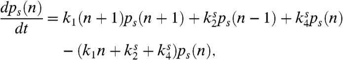
Fig. 1.

A cellular network for the computation of an external ligand concentration. External ligands are detected by a receptor that can exist in two conformations: A high-activity on state and a low-activity off state. Receptors switch between states at rate k_off and k_on. Receptors in state s = {on,off} can post-translationally activate (i.e., phosphorylate) a downstream protein at a rate . The protein is deactivated (i.e., dephosphorylated) at a constant rate k₁.

Here, we consider a simple two-component biochemical network that encodes information about ligand concentration in the steady-state concentration of the activated form of a downstream protein (as shown in Fig. 1). Such two-component networks are a common signal transduction motif found in bacteria and are often used to sense external signals through receptor-catalyzed phosphorylation of a downstream response regulator (16). The membrane-bound receptors can be in an either an active “on” state or an inactive “off” state. For simplicity, as in previous works (12–14), we assume that the binding affinity of the on state is extremely high such that all ligand-bound receptors are always in the on state and all unbound receptors are in the off state. Receptors can switch between the off state and on state at a concentration-dependent rate and from the on state to the off state at a concentration-independent rate . Receptors additionally convert a downstream signaling protein from an inactive form X to an active form X^∗, by, for example, phosphorylation, at a state-dependent rate , where s = on,off. The proteins are deactivated at a state-independent rate k₁. The dependence of on the receptor state is what propagates information about ligand concentration downstream. The biochemical network described above contains all the basic elements of a computing device (see Table 1).

Table 1.

Summary of the biological realization of basic computational elements

Computational element	Biological realization
Memory	Number of activated (phosphorylated) proteins
Writing to memory	Concentration dependent activation (phosphorylation) of proteins
Erasure of memory	Deactivation (dephosphorylation) of proteins
Energy dissipation	Entropy production due to a lack of detailed balance in chemical kinetic of activation/deactivation

Importantly, the deactivation rate of the off state is small yet must be nonzero for thermodynamic consistency (17). We also note that for the case where proteins are activated through phosphorylaltion, includes nonspecific phosphorylation arising from other kinases as well as contributions from the reverse reactions of the phosphotases. The inactivation rate sets the scale for the effective measurement time because it is the rate at which information encoded in downstream proteins is lost due to inactivation. In order to compute external concentrations accurately, the measurement time must be much longer than the typical switching times between receptor states, . We show below that this simple network in fact implements a noisy version of the original Berg–Purcell calculation. Our explicit construction allows us to study the relationship between information and power consumption in this network.

The paper is organized as follows. In the first section, we compute the steady-state behavior of the system, first within the linear-noise approximation and then through an exact solution of the corresponding master equation. In the next two sections, we quantify the efficacy of chemosensation through the variance in estimated concentration (using the linear-noise approximation) and calculate the power consumption required to maintain the network in steady state (using the exact solution). Finally, we show there exists a tradeoff between these two quantities and discuss implications for the design of cellular sensing systems. We begin each section with a general discussion that summarizes the major ideas, results, and interpretations followed by a more technical and mathematical discussion.

Characterization of the Network’s Steady-State Properties

In this section, we derive the steady-state properties of the cellular network considered above. The network translates the external ligand concentration into an internal concentration of activated proteins. This mapping between external ligand concentration and downstream protein number is probabilistic due to the stochasticity inherent in biochemical networks. For this reason, we can characterize the output of the network by a probability distribution of activated proteins, p(n). The shape of the distribution p(n) depends explicitly on the kinetic parameters (k₁, , ) (see Fig. 2). In the following sections, we focus on the fast-switching regime where receptors switch between the on and off states quickly as compared to the deactivation rate, and as we will see, p(n) is unimodal (see Fig 2B).

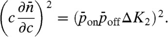
Fig. 2.

Top Slow switching regime, , with a bimodal distribution of activated proteins. Probability of having n activated proteins at steady-state (black solid line), probability of having n activated proteins when receptor is in the on state (blue dash-dot line), probability of having n activated proteins when receptor is in the off state (red dashed line). Middle Fast switching regime, , where the distribution of activated proteins is unimodal. Total probability (black solid line), probability when receptor is in the on state (blue dash-dot line), probability when receptor is in the off state (red dashed line). Bottom The uncertainty in ligand concentration, 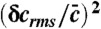as a function of k₁ with mean number of active proteins (dashed red line) and . This can be compared to the Berg–Purcell result (solid black line). Parameters: , .

In this regime, two important characteristics of the distribution p(n) are the mean, protein number, , and variance . The mean protein number is the cell’s best estimate of the external ligand concentration. On the other hand, the variance characterizes the cell’s uncertainty about external ligand concentrations due to stochasticity in the underlying biochemical network. Though it is possible to decrease the variance by increasing the mean protein number, it will be always be nonzero due to fluctuations in the state of the receptors (12).

We begin by first deriving the steady-state mean and variance of the number of activated proteins, n, within the linear-noise approximation. Afterwards, we will study the full probability distribution. The deterministic dynamics of the biochemical network in Fig. 1 is captured by simple rate-equations for the time dependence of the receptor state probabilities and the mean number of activated proteins. We can augment these equations to account for stochastic fluctuations within the linear-noise approximation by adding appropriate Langevin noise terms. In the remainder of this paper, we assume for simplicity that proteins are abundant and ignore saturation effects. The dynamics of the circuit is therefore described by a pair of Langevin equations for the probabilities p_on and p_off (i.e. 1 - p_on) for the receptor to be in the on or off states, respectively, together with the number of activated proteins n,

[1]

[2]

The variance of the Langevin terms is given by the Poisson noise in each of the reactions:

[3]

where δ(t - t^′) denotes the Dirac-delta function and the overbar denotes the mean steady-state value of the respective quantity (18, 19).

At steady-state, we can calculate the mean probability and number of proteins by setting the time derivative in Eq. 2 equal to zero while ignoring noise terms, yielding

[4]

and

[5]

where we have defined the dimensionless parameters with j = {2,4} and s = {on,off}. For the biologically realistic case , the mean number of proteins is simply proportional to the kinase activity in the on state times the probability of being in the on state, , as expected. One can further calculate the variance in protein numbers (SI Text)

[6]

The first term on the right-hand side of the equation results from Poisson noise in the synthesis and degradation of activated protein, whereas the second term is due to stochastic fluctuations in the state of the receptors.

In addition to the mean and variance, we will need the full steady-state probability distribution for n to calculate the power consumption of the network. The steady-state distribution can be calculated from the master equation for the probability, p_s(n), of there being n active proteins with the receptor in a state s:

[7]

where (on) when s = on (off). This equation is similar to those found in (20, 21) and the steady-state distribution can be solved via a generating function approach (see SI Text).

Depending on the parameters, the steady-state distributions can have two qualitatively distinct behaviors as shown in Fig. 2. In the “slow switching” regime with and , receptors switch at rates much slower than the protein deactivation rate k₁. The result is a bimodal distribution of activated proteins that can be intuitively understood to arise from the superposition of the probability distributions of activated proteins when the receptor is the on and off states. Similar behavior has been found in the steady-state expression of a self-regulation of a gene (22). As approaches , the distributions in the two states merge and the overall probability distribution becomes unimodal. On the other hand, in the “fast switching” regime, characterized by 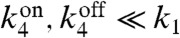, the distribution of activated proteins is always unimodal. In this limit, the measurement time, 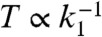, is much longer than the average time a receptor remains in the on or off state, and the biochemical network “time-averages” out the stochastic fluctuations in receptor states. In what follows, we restrict our considerations to this latter regime.

Quantification of Learning

The biochemical circuit in Fig. 1 “computes” the external concentration of a chemical ligand. As emphasized by Berg and Purcell in their seminal paper (12), the chief obstacle in determining external concentration is the stochastic fluctuations in the state of the ligand-binding receptors. Berg and Purcell argued that a reasonable measure of how much cells learn is the uncertainty cells have about external concentration as measured by the variance of the estimated concentration, (δc)². (δc)² measures the uncertainty about the external ligand concentration based on the probability distribution of downstream activated proteins. Using standard arguments, we show below that this uncertainty is directly related to the variance, (δn)², of the corresponding protein probability distribution. This framework allows us to use the results of the last section to quantify how much cells learn about external ligand concentrations as a function of kinetic parameters. The results are plotted in Fig. 2C.

To compute uncertainty, Berg and Purcell assumed that the cell computes the average receptor occupancy by time-averaging over a measurement time T. They showed (12) that

[8]

where , is independent of c, and N_b is the number of binding events during the time T. It was later shown that cells could compute concentration more accurately by implementing MLE with (14, 23)

[9]

The factor of two decrease in uncertainty derives from the fact that MLE ignores noise due to unbinding of ligands from the cell. We note that this "forgetting" of ligand unbinding, in turn, requires the receptors themselves to be out of equilibrium, further contributing to the system’s energy consumption. We do not, however, consider the additional energetic costs of nonequilibrium receptors here.

To quantify learning in our biochemical circuit, we follow Berg and Purcell and estimate the fluctuations in (δc)² as

[10]

with . Substituting and 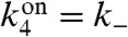and computing the derivative using Eq. 5 gives

[11]

Substituting Eqs. 5 and 6 into Eq. 10 yields

[12]

Similar to the linear-noise calculation, the first term on the right-hand side arises from the Poisson fluctuations in activated protein number, while the second term results from the stochastic fluctuations in the state of receptors. Fig. 2 shows the uncertainty, (δc)²/c², as a function of the degradation rate of activated protein, k₁, when and and .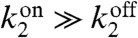

By identifying the degradation rate with the inverse measurement time, k₁ = 2T^-1, we can also compare the results with Berg–Purcell. The factor of two is due to the slight difference in how the variance of the average receptor occupancy is calculated for a biochemical network when compared to the original Berg–Purcell calculation (23). As shown in Fig. 2, when is increased, the Poisson noise in protein production is suppressed and the performance of the cellular network approaches that due to Berg-Purcell. To make the connection with Berg–Purcell more explicit, it is helpful to rewrite Eq. 12 in terms of the average number of binding events, N_b, during the averaging time, T:

[13]

This form allows us to see the approach to the Berg–Purcell limit. When the measurement time is much longer than the timescale of fluctuations in receptor activity, i.e., (or equivalently ) and the average number of activated proteins is large, 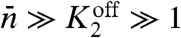, the expression above reduces to (δc)²/c² ≈ 2/N_b in agreement with Eq. 8.

Power Consumption and Entropy Production in Steady State

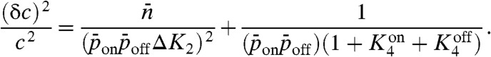
We now compute the energy consumed by the circuit in Fig. 1 as a function of the kinetic parameters. To do so, we exploit the fact that dynamics of the circuit can be formulated as a nonequilbrium Markov process (see Fig. 3). A nonequilibrium steady-state (NESS) necessarily implies the breaking of detailed balance in the underlying Markovian dynamics and, therefore, possesses a nonzero entropy production rate. The entropy production rate is precisely the amount of power consumed by the biochemical circuit in maintaining the nonequilibrium steady state. Thus, by calculating the entropy production rate as function of kinetic parameters, we can calculate the power consumed by the biochemical network implementing the computation. To calculate entropy production, we utilize the full steady-state probability distribution and standard formulas from the theory on nonequilibrium Markov processes.

Fig. 3.

Upper The probabilistic Markov process underlying the circuit in Fig. 1 takes the form of a two-legged ladder. Any nonzero cyclic flux (depicted in red) results in entropy production and power consumption. Lower Power consumption (solid black line) and uncertainty (dashed purple line) as a function of 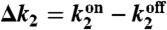when , and .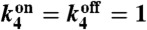

Consider a general Markov process with states labeled by σ and transition probability from σ to σ^′ given by k(σ,σ^′). Defining the steady-state probability of being in state σ by P_σ, the entropy production rate, EP, for a NESS is given by (24)

[14]

For our problem this general formula reduces to

[15]

where we again use (see SI Text). In deriving this formula, we assumed that the receptors were in thermal equilibrium and obeyed detailed balance. Using explicit expressions for the steady-state distributions, p_s(n), we can calculate the energy consumption of the network as a function of kinetic parameters (see SI Text). The physical content of this expression is summarized in Fig. 3. The expression states that any nonzero cyclic flux must necessarily produce entropy. Otherwise, one would have a chemical version of a perpetual motion machine. Figs. 3 and 4 show the power consumption as a function of 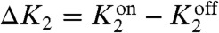and k₁. Notice that the power consumption tends to zero as both these parameters go to zero. Note that we cannot, however, set k₁ = 0 identically because there then no longer exists a steady-state distribution.

Fig. 4.

Total energy per independent measurement () as a function of k₁ when . (Inset) Power consumption as a function of k₁ over the same parameter range. Note that although the system’s power consumption decreases with decreasing k₁, the energy per measurement increases.

Energetics, Information, and Landauer’s Principle

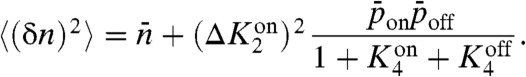
We now highlight the fundamental connection between the energy consumed by the network and the information the network acquires about the environment and briefly discuss its relation to Landauer’s principle. First, note that learning information about the environment requires energy consumption by the network. This relationship can be seen in Fig. 3, which shows that as Δk₂ → 0, the uncertainty about the concentration tends to infinity. Moreover, we show in the SI Text that the entropy production, Eq. 15, is zero if and only if Δk₂ = 0. In conjunction with Eq. 12, which diverges as Δk₂ → 0, these observations imply that learning requires consuming energy. Mathematically, in the limit where Δk₂ = 0, the dynamics of the Markov process in Fig. 3 become “one-dimensional” instead of a two-legged ladder, and the dynamics obeys detailed balance. Physically, in this limit the number of downstream proteins becomes insensitive to external ligand concentrations because all information about concentration is contained in the relative probabilities of being in the on or off state.

Second, as shown in Fig. 4, the power consumption of the circuit tends to zero as k₁ → 0. This result is consistent with, and a manifestation of, Landauer’s principle: Entropy production stems from erasing memory in a computing device. The number of activated proteins serves the function of a memory of ligand concentration, which is erased at the dephosphorylation rate k₁. Thus, as the erasure rate of the memory tends to zero, the device consumes less energy per unit time, as expected. Yet despite the fact that the power consumption tends to zero as k₁ decreases, the total energy consumed per measurement, namely the power times the measurement time, , still increases (see Fig. 4). Thus, learning more requires consuming more total energy despite the fact that power consumption is decreasing. In effect, one is approaching the reversible computing limit where memory is erased adiabatically. Again note, however, that when erasure is performed infinitely slowly, k₁ = 0, the system no longer has an NESS and our formalism does not apply.

Finally, we note that one of the important open problems in our understanding of chemosensation is a full characterization of the constraints placed on the measurement time T. In principle, cells can always learn more by measuring the environment for longer periods of time. However, in most biological systems, these measurement times are observed to be quite short. There are a number of constraints that can limit this measurement time, including rotational diffusion (12) (in the case of swimming bacteria) and the restrictions placed on motility. Here, we highlight another restriction that may be important in resource-starved environments: Sensing external concentration necessarily requires cells to consume energy.

Discussion and Conclusion

Cells often perform computations using elaborate biochemical networks that respond to environmental cues. One of the most common simple networks found in bacteria are two-component networks where a receptor phosphorylates a downstream response regulator (16). In this work, we have shown that these simple two-component networks can implement a noisy version of the Berg–Purcell strategy to compute the concentration of external ligands. Furthermore, by mapping the dynamics of the biochemical network to nonequilibrium steady-states in Markov processes, we explicitly derived expressions for the power consumed by the network and showed that learning requires energy consumption. Taken together, these calculations suggest that, much like man-made and neural computing (3, 9–11), energetic considerations may place important constraints on the design of biochemical networks that implement cellular computations. They also suggest a fundamental tradeoff between the efficiency of cellular computing and the requisite energy consumption.

Bacterial cells such as Bacillus subtilis can sporulate during times of environmental stress and remain metabolically dormant for many years. Although sporulation is relatively well understood, the reverse process of germination is much more difficult to study. One current model for how a spore knows when to germinate in response to external cues involves integrating the signal and triggering commitment when an accumulation threshold is reached (25, 26). Such a scheme corresponds to the limit of vanishingly small k₁ in our model, so that power consumption is minimized at the expense of retaining the entire integrated signal. Our results indicate that this behavior may be due to the extreme energetic constraints imposed on a metabolically dormant spore, rather than an evolutionarily optimized strategy.

An important insight of this work is that even a simple Berg–Purcell strategy for sensing external concentrations requires the consumption of energy. It is likely that more complicated strategies that increase how much cells learn, such as maximum likelihood, require additional energetic inputs. For example, it was argued in (23) that MLE can be implemented by a network similar to the perfect adaptation network where bursts are produced in response to binding events. These bursts break detailed balance and therefore require energy consumption. It will be interesting to investigate further how the tradeoff between learning and energy consumption manifests itself in the design of computational strategies employed by cells.

In this work, we restricted ourselves to the simple case where cells calculate the steady-state concentration of an external signal. In the future, it will be useful to generalize the analysis performed here to other computations such as responding to temporal ramps (23) and spatial gradients (27, 28). It will also be interesting to understand how to generalize the considerations here to arbitrary biochemical networks. An important restriction on our work is that we reduced our considerations to nonequilibrium steady states. It will be interesting to ask how to generalize the work here to biochemical networks with a strong temporal component.

References

- 1.Landauer R. Irreversibility and heat generation in the computing process. IBM J Res Dev. 1961;5:183–191. [Google Scholar]
- 2.Berut A, et al. Experimental verification of Landauers principle linking information and thermodynamics. Nature. 2012;483:187–189. doi: 10.1038/nature10872. [DOI] [PubMed] [Google Scholar]
- 3.Bennett C. The thermodynamics of computation: A review. Int J Theor Phys. 1982;21:905–940. [Google Scholar]
- 4.Del Rio L, Berg J, Renner R, Dahlsten O, Vedral V. The thermodynamic meaning of negative entropy. Nature. 2011;474:61–63. doi: 10.1038/nature10123. [DOI] [PubMed] [Google Scholar]
- 5.Qian H, Reluga T. Nonequilibrium thermodynamics and nonlinear kinetics in a cellular signaling switch. Phys Rev Lett. 2005;94:28101. doi: 10.1103/PhysRevLett.94.028101. [DOI] [PubMed] [Google Scholar]
- 6.Qian H. Thermodynamic and kinetic analysis of sensitivity amplification in biological signal transduction. Biophys Chem. 2003;105:585–593. doi: 10.1016/s0301-4622(03)00068-1. [DOI] [PubMed] [Google Scholar]
- 7.Lan G, Sartori P, Neumann S, Sourjik V, Tu Y. The energy-speed-accuracy trade-off in sensory adaptation. Nat Phys. 2012;8:422–428. doi: 10.1038/nphys2276. [DOI] [PMC free article] [PubMed] [Google Scholar]
- 8.Tu Y. The nonequilibrium mechanism for ultrasensitivity in a biological switch: Sensing by Maxwell’s demons. Proc Natl Acad Sci USA. 2008;105:11737–11741. doi: 10.1073/pnas.0804641105. [DOI] [PMC free article] [PubMed] [Google Scholar]
- 9.Laughlin S. Energy as a constraint on the coding and processing of sensory information. Curr Opin Neurobiol. 2001;11:475–480. doi: 10.1016/s0959-4388(00)00237-3. [DOI] [PubMed] [Google Scholar]
- 10.Laughlin S, van Steveninck R, Anderson J. The metabolic cost of neural information. Nat Neurosci. 1998;1:36–41. doi: 10.1038/236. [DOI] [PubMed] [Google Scholar]
- 11.Balasubramanian V, Kimber D, II M. Metabolically efficient information processing. Neural Comput. 2001;13:799–815. doi: 10.1162/089976601300014358. [DOI] [PubMed] [Google Scholar]
- 12.Berg H, Purcell E. Physics of chemoreception. Biophys J. 1977;20:193–219. doi: 10.1016/S0006-3495(77)85544-6. [DOI] [PMC free article] [PubMed] [Google Scholar]
- 13.Bialek W, Setayeshgar S. Physical limits to biochemical signaling. Proc Natl Acad Sci USA. 2005;102:10040–10045. doi: 10.1073/pnas.0504321102. [DOI] [PMC free article] [PubMed] [Google Scholar]
- 14.Endres R, Wingreen N. Maximum likelihood and the single receptor. Phys Rev Lett. 2009;103:158101. doi: 10.1103/PhysRevLett.103.158101. [DOI] [PubMed] [Google Scholar]
- 15.Magnasco M. Chemical kinetics is turing universal. Phys Rev Lett. 1997;78:1190–1193. [Google Scholar]
- 16.Laub M, Goulian M. Specificity in two-component signal transduction pathways. Annu Rev Genet. 2007;41:121–145. doi: 10.1146/annurev.genet.41.042007.170548. [DOI] [PubMed] [Google Scholar]
- 17.Beard D, Qian H. Chemical biophysics: Quantitative analysis of cellular systems. Cambridge, MA: Cambridge Univ Press; 2008. [Google Scholar]
- 18.Detwiler P, Ramanathan S, Sengupta A, Shraiman B. Engineering aspects of enzymatic signal transduction: Photoreceptors in the retina. Biophys J. 2000;79:2801–2817. doi: 10.1016/S0006-3495(00)76519-2. [DOI] [PMC free article] [PubMed] [Google Scholar]
- 19.Mehta P, Goyal S, Wingreen N. A quantitative comparison of sRNA-based and protein-based gene regulation. Mol Syst Biol. 2008;4:221. doi: 10.1038/msb.2008.58. [DOI] [PMC free article] [PubMed] [Google Scholar]
- 20.Iyer-Biswas S, Hayot F, Jayaprakash C. Stochasticity of gene products from transcriptional pulsing. Phys Rev E. 2009;79:031911. doi: 10.1103/PhysRevE.79.031911. [DOI] [PubMed] [Google Scholar]
- 21.Visco P, Allen R, Evans M. Statistical physics of a model binary genetic switch with linear feedback. Phys Rev E. 2009;79:031923. doi: 10.1103/PhysRevE.79.031923. [DOI] [PubMed] [Google Scholar]
- 22.Hornos JE, et al. Self-regulating gene: An exact solution. Phys Rev E. 2005;72 doi: 10.1103/PhysRevE.72.051907. [DOI] [PubMed] [Google Scholar]
- 23.Mora T, Wingreen N. Limits of sensing temporal concentration changes by single cells. Phys Rev Lett. 2010;104:248101. doi: 10.1103/PhysRevLett.104.248101. [DOI] [PubMed] [Google Scholar]
- 24.Lebowitz J, Spohn H. A gallavotti–cohen-type symmetry in the large deviation functional for stochastic dynamics. J Stat Phys. 1999;95:333–365. [Google Scholar]
- 25.Yi X, Liu J, Faeder J, Setlow P. Synergism between different germinant receptors in the germination of Bacillus subtilis spores. J Bacteriol. 2011;193:4664–4671. doi: 10.1128/JB.05343-11. [DOI] [PMC free article] [PubMed] [Google Scholar]
- 26.Indest K, Buchholz W, Faeder J, Setlow P. Workshop report: Modeling the molecular mechanism of bacterial spore germination and elucidating reasons for germination heterogeneity. J Food Sci. 2009;74:R73–R78. doi: 10.1111/j.1750-3841.2009.01245.x. [DOI] [PubMed] [Google Scholar]
- 27.Endres R, Wingreen N. Accuracy of direct gradient sensing by single cells. Proc Natl Acad Sci USA. 2008;105:15749–15754. doi: 10.1073/pnas.0804688105. [DOI] [PMC free article] [PubMed] [Google Scholar]
- 28.Hu B, Chen W, Rappel W, Levine H. Physical limits on cellular sensing of spatial gradients. Phys Rev Lett. 2010;105:48104. doi: 10.1103/PhysRevLett.105.048104. [DOI] [PMC free article] [PubMed] [Google Scholar]
Associated Data
This section collects any data citations, data availability statements, or supplementary materials included in this article.