Emergence of Selectivity and Tolerance in the Avian Auditory Cortex

Abstract

The ability to recognize auditory objects like words and bird songs is thought to depend on neural responses that are selective between categories of the objects and tolerant of variation within those categories. To determine whether a hierarchy of increasing selectivity and tolerance exists in the avian auditory system, we trained European starlings (Sturnus vulgaris) to differentially recognize sets of songs, then measured extracellular single unit responses under urethane anesthesia in six areas of the auditory cortex. Responses were analyzed with a novel, generalized linear mixed model that provides robust estimates of the variance in responses to different stimuli. There were significant differences between areas in selectivity, tolerance, and the effects of training. The L2b and L1 subdivisions of field L had the least selectivity and tolerance. The caudal nidopallium (NCM) and subdivision L3 of field L were more selective than other areas, whereas the medial and lateral caudal mesopallium were more tolerant than NCM or L2b. L3 had a multimodal distribution of tolerance. Sensitivity to songs that were familiar and those that were not also distinguished the responses of caudomedial mesopallium and NCM. There were significant differences across areas between neurons with wide and narrow spikes. Collectively these results do not fit the traditional hierarchical view of the avian auditory forebrain, but are consistent with emerging concepts homologizing avian cortical and neocortical circuitry. The results suggest a functional divergence within the cortex into processing streams that respond to complementary aspects of the variability in communicative sounds.

Introduction

Neurons in higher, more central areas of sensory processing pathways tend to have more complex response properties as compared with the periphery, including larger, more nonlinear receptive fields (Hubel and Wiesel, 1965; Sen et al., 2001; Escab í and Read, 2003; David et al., 2006); stronger preference for behaviorally relevant stimuli (Leppelsack and Vogt, 1976; Suga, 1978; Desimone et al., 1984; Müller and Leppelsack, 1985); greater selectivity between stimuli of similar complexity (Margoliash, 1986; Kobatake and Tanaka, 1994; Logothetis et al., 1995; Rust and DiCarlo, 2012); and greater tolerance for noise, clutter, and other irrelevant sources of variability (Rolls, 2000; Zoccolan et al., 2007). Selectivity and tolerance are thought to be important for recognizing objects and categories of stimuli (Riesenhuber and Poggio, 2002), and to reflect learning about which sources of variation carry behaviorally relevant information and which do not (Sigala and Logothetis, 2002; Freedman and Assad, 2006).

Auditory systems exhibit hierarchically organized increases in receptive field size and nonlinearity (Sen et al., 2001; Escab í and Read, 2003; Nagel and Doupe, 2008), but the hierarchical organization of stimulus selectivity and tolerance is not as well established. Some auditory signals, like words and phonemes, form natural categories: they are perceived as distinct entities despite substantial variation in how they are produced by different speakers or in different contexts (Hillenbrand et al., 1995). Many bird species also produce complex vocalizations that have distinct behavioral meanings (Falls, 1982; Sharp et al., 2005) even though they vary acoustically from rendition to rendition. For example, European starling (Sturnus vulgaris) songs consist of a sequence of temporally discrete “motifs” (Adret-Hausberger and Jenkins, 1988; Eens et al., 1989). Each starling has a unique repertoire of distinct motif types, which are used in many songs and often repeated in the same song. Motif types are relatively stereotyped, but renditions vary in pitch, duration, and other acoustic features (Gentner, 2004). In behavioral tasks, starlings recognize the songs of other individuals on the basis of motif types while ignoring variability between renditions (Gentner and Hulse, 1998; Gentner, 2004).

Here we examined whether neural selectivity and tolerance emerge at cortical levels of the starling auditory system by recording from six different areas of the auditory pallium, the presumptive homolog to mammalian auditory neocortex (Reiner et al., 2004; Wang et al., 2010; Dugas-Ford et al., 2012). Three areas were subdivisions of field L, the primary thalamorecipient zone (Karten, 1968), and the other three were the caudal nidopallium (NCM), the caudolateral mesopallium (CLM), and the caudomedial mesopallium (CMM) (Fig. 1; Vates et al., 1996), which receive input from field L and exhibit learning-dependent responses (Gentner and Margoliash, 2003; Thompson and Gentner, 2010; Jeanne et al., 2011). Single unit responses were recorded to presentations of conspecific songs, some of which were learned in an auditory discrimination task. We developed a novel modeling methodology to evaluate selectivity, tolerance, and the effects of learning from the distribution of the neural responses across the presented motif types and variants.

Figure 1.

Auditory areas of the avian cortex. Outlines are traced from two parasagittal sections from a European starling at 0.6 mm (a) and 1.8 mm (b) from the midline. Dashed lines indicate boundaries that are defined by gradual transitions between cytoarchitectures. L2a and L2b (light gray) are the primary thalamorecipient areas. Arrows represent connections between areas as described in zebra finches (Vates et al., 1996) and pigeons (Wild et al., 1993); darker arrows indicate connections within larger subdivisions. Hp, hippocampus; LaM, lamina mesopallialis; LAD, lamina arcopallialis dorsalis; all other areas are subdivisions of field L.

Materials and Methods

Fourteen adult European starlings of both sexes (three male, six female, five unknown) were captured from farms in northeastern Illinois or at O'Hare Airport. They were housed in mixed-sex flight aviaries and received food and water ad libitum. The lighting schedule was matched to local daylight hours in Chicago. All animal procedures were performed according to protocols approved by the University of Chicago Institutional Animal Use and Care Committee and consistent with the guidelines of the National Institutes of Health.

Stimuli.

Songs were recorded from three adult male starlings captured and housed under similar conditions as the experimental subjects, but at a much earlier date, with no overlap in tenancy. During recording each bird was housed in isolation, in a 2 m³ double-walled sound isolation booth (Industrial Acoustics). Recordings were made with an AT4071a directional microphone (Audio-Technica) and amplified with a DMP3 microphone preamplifier (M-Audio). Signals were digitized with a DB2000 PCI digital acquisition board (Measurement Computing) with a sampling rate of 20 kHz and resolution of 16 bits per sample, without an anti-aliasing filter. Songs were stored to disk, digitally highpass filtered (12 dB/octave) at 100 Hz, and scaled to 96 dB peak amplitude. Between 100 and 300 complete song bouts were recorded from each bird over the course of several days.

From the song bouts recorded for each bird, 10 representative segments of about 10 s each (hereinafter songs) were extracted, sampling equally from the beginnings, middles, and ends of the bouts. Each song was manually segmented into motifs (11–17 per song segment; median 13.5) based on visual examination of the spectrograms. Motifs are temporally discrete vocal elements between 500 and 1200 ms in length composed of a fairly stereotyped pattern of notes (Eens et al., 1989). We grouped the recorded motifs into types based on note-level similarity, with the rule that motifs sharing <50% of their notes in common, or in which the notes were sung in a markedly different order, were considered different types. In the text to follow, “motif type” and “motif variant” are used to refer to this scheme, whereas motif is used in a more generic sense to refer to a specific recording of a variant but ignoring its type. The term “category” is used exclusively to refer to a behavioral response category imposed by operant training (see next section), or to whether a motif is familiar or unfamiliar. The 373 motifs recorded from all three singers comprised 107 unique types, with 1–13 variants of each type (median 3).

Behavioral training.

Starlings were operantly trained to recognize songs following previously described procedures (Gentner and Margoliash, 2003). Briefly, after the bird probed a detection port to start a trial, one of the song stimuli was presented. After stimulus playback, there was a 2 s window when responses were rewarded with food or punished with a 10 s period when the lights were extinguished and no trials could be initiated. Three sets of stimuli each consisted of six songs from one of the singers. For birds trained on a go-no-go paradigm (n = 12/14), one set was designated as “S+,” meaning that responses were rewarded, and another set was designated as “S−,” meaning that responses were punished. Failure to respond was neither punished nor rewarded. Two birds were trained on a two-alternative-choice paradigm, which required them to peck one of two keys during the response period. One set of stimuli was assigned to each key, and the birds were rewarded if their choice was correct and punished if it was not. The third song set was not presented to the bird at any time before electrophysiological recording. Training was balanced across subjects so that each set was familiar to some birds and unfamiliar to others.

Each bird was trained on the task until it reached an average accuracy of at least 85% over three consecutive blocks of 100 trials. Stimuli were presented randomly with replacement, except during trials after an incorrect response, when the stimulus was the same as on the previous trial. These correction trials help to speed learning and reduce response bias. Discrimination performance was plotted using d-prime (Macmillan et al., 1977), d′ = z(p_hit) − z(p_fa), where z is the z-score, and p_hit and p_fa are the proportion of hit and false alarm responses in the block.

Electrophysiology.

After the birds reached criterion behavioral performance, an annular metal chamber used for head fixation was surgically implanted under anesthesia, either Equithesin (3.75 mL/kg, i.m.) or isoflurane gas (1–2% by volume in air). The scalp and upper layer of skull were removed over the caudal forebrain, and the implant was affixed to the skull using dental acrylic. Birds were allowed to recover in isolation for several days before beginning recording. On recording days, birds were food deprived and anesthetized with urethane (20% by volume, 5 mL/kg, i.m.).

Recordings from field L, NCM, CLM, and CMM in both hemispheres were made using 16-channel single shank silicon multi-electrode arrays with 413 μm² or 117 μm² recording sites separated by 50 μm (models A1x16–5mm50–413 and A1x16–5mm50–117; NeuroNexus Technologies). Recordings were in 1–3 areas per bird (median 2), and each area was recorded in 4–7 birds (median 4.5). Signals were amplified and bandpass filtered between 300 and 3000 Hz (Model 15; Neurodata, Grass Instruments), digitized at 20 kHz (DB3000; Measurement Computing), and stored to computer disk. The spiking responses of single units were extracted from recordings using principal-components-based sorting. Spike clusters were first calculated automatically using KlustaKwik and then manually refined with Klusters (K. Harris, L. Hazan, G. Buzsáki lab, Rutgers, Newark, NJ) (Hazan et al., 2006). A unit was considered to be well isolated only if <0.1% of the interspike intervals were <1 ms and the cluster was significantly separated in the principal component space from all other clusters and the unsorted noise (MANOVA: p < 0.05). Neurons in L2a are small and highly clustered (Fortune and Margoliash, 1992), and only one unit from L2a was sufficiently isolated to meet these criteria, so this area was not included.

Due to the linear geometry of the electrodes, the same unit was sometimes recorded on a different channel after the electrode had been advanced to a new site. Whenever well isolated units were recorded within 25 μm of a previously recorded unit (n = 39), the responses to stimuli presented at both sites (6–24 songs, median = 6) were visually compared to determine whether both recordings had the same response properties (spike shape, average rate, phasicness, etc.) and temporal patterns of evoked activity. In 24/39 cases the responses were essentially identical, and the trials from the two sites were considered as a single unit. In the remaining cases the trials were considered as coming from separate units. Neurons were categorized as wide spike or narrow spike by averaging the spikes for each unit, aligning their peaks, and using affinity propagation clustering (Frey and Dueck, 2007) on the first two principal components (PCs). There were two large clusters in the PC space, one corresponding to spikes with a narrow peak and a narrow, deep trough (hereafter, narrow spikes) and the other to spikes with a broader peak and a broad, shallow trough (wide spikes). Spike shapes for all neurons are shown in Figure 4b. A few neurons in CLM and CMM exhibited a sharp initial dip before the peak of the spike but were otherwise like the wide-spike neurons and were treated as such for this study. The two neuronal classes were well separated in the principal components space (MANOVA: p < 10⁻¹⁵).

Figure 4.

Motif selectivity of wide- and narrow-spike neurons in cortical auditory areas. a, Cumulative distributions of average firing rate evoked by the motifs presented to each neuron (gray lines). Distributions are normalized by the maximum response. Cyan lines correspond to exemplar neurons from Figure 3, and the thick red and blue lines are the average of the distributions for the narrow- and wide-spike neurons in each area. b, Average spike shapes for narrow-spike (red traces) and wide-spike neurons (blue traces). c, Projections of spike waveforms for each neuron onto the first two principal components of the spike shape. d, AF (selectivity) by area and spike type. Areas have been ordered to emphasize increasing selectivity. Circles represent individual neurons, which have been horizontally jittered for clarity. Error bars indicate mean ± SE. NCM and L3 have higher selectivity than the other areas (*p < 0.05), and selectivity is higher for wide-spike neurons (p = 0.01).

Stimuli were presented free-field in an anechoic chamber (IAC-3) from a speaker positioned in front of the bird, at an root mean square amplitude of 67–70 dB sound pressure level, measured from the position of the bird's head. All 18 training songs plus 6 additional songs, representing a total of 296 unique motifs, were used when searching for responsive units. Once sufficient isolation of a single unit was achieved on at least one channel, responses to between 5 and 50 repetitions (median 10) of one or more songs were recorded. For some neurons, 6–19 songs (familiar and unfamiliar) were presented in random order. For other neurons, one of the songs was presented along with stimuli derived from the song, which were used in a different study (Meliza et al., 2010); up to three songs (chosen pseudorandomly to ensure equal sampling of songs from each singer) were tested in this way for as long as the recording remained stable. The number of unique motif types tested on a neuron ranged from 5 to 90 (median 20), with a median of 2 variants per type (range 1–9).

Responses were analyzed by dividing them into intervals corresponding to the component motifs of the song stimuli and counting the number of spikes that occurred in each interval. The intervals spanned from the onset of each motif to the onset of the following motif. (The last interval in the song ended at the offset of the last motif, plus an interval equal to the average gap between motifs in the song.) The number of spikes that occurred during a baseline silent period 2000 ms before the onset of the stimulus was also counted. Motifs were coded as “familiar” if they had been presented in the operant training and “unfamiliar” if they had not. The same analyses were repeated with motifs coded for response association (i.e., S+, S−, unfamiliar; or left, right, unfamiliar), but this greatly reduced statistical power and we failed to find significant differences between familiar response categories.

Histology.

At the end of the recording session, one or two fiduciary lesions were made, and birds were given an overdose of Nembutal (250 mg/kg) and transcardially perfused with heparinized saline followed by 10% formalin. The brains were cryoprotected in 30% sucrose formalin until saturated (2–4 d). Tissue was sectioned at 50 μm parasagittally using a cryostat and stained with cresyl violet. The locations of the recording sites were assigned to areas CMM, CLM, NCM, L1, L3, or L2b, generally following the divisions outlined by Fortune and Margoliash (1992; Fig. 1). Neurons with ambiguous locations were excluded from further analysis (58/431 auditory units). The majority of the excluded neurons came from the border of L2b and L3 (n = 30), where the larger, more widely spaced neurons that distinguish L3 emerge gradually. Neurons from the portion of NCM dorsal to L2b and caudal of CM (n = 13) were also excluded. We deliberately avoided recording near the rostrocaudal boundary of L2b and NCM and the mediolateral boundary of CLM and CMM, which are also gradual. The division between CLM and CMM was taken to be the first section in which L2a could be distinguished (usually 1.0–1.2 mm from the midline). All sites were at least 0.1 mm from the center of any gradual boundary. Some L2b sites may be from the L subdivision (Fortune and Margoliash, 1992), which has cytoarchitecture similar to L2b but is not thought to receive direct thalamic input. Within NCM, 37/50 units (74%) were from the dorsal half. A dorsal/ventral physiological distinction has been noted for NCM (Vates et al., 1996; Thompson and Gentner, 2010).

Measures of selectivity and tolerance.

Neuronal selectivity was initially quantified using a nonparametric measure called activity fraction (AF) or sparseness (Vinje and Gallant, 2000; Lehky et al., 2005), an index calculated from the response of a neuron to each of N stimuli. We used the formula $A=\frac{1-{\left({\displaystyle \sum r_i/N}\right)}^2/{\displaystyle \sum r_i^2/N}}{1-1/N}$, where r_i is the rate of the neuron's response to stimulus i, averaged across trials.

To quantify the degree to which selectivity was due to differences between motif types (between-type) versus differences between variants of the same type (within-type), we used a generalized linear mixed-effects model (GLMM) (Gelman and Hill, 2006). GLMMs are commonly used in ecology and psychology but their application in neuroscience is relatively new, so a detailed description follows.

In essence, a GLMM is a linear regression model in which (1) the distribution of the response variable does not have to be Gaussian and (2) the regressors can modeled as random effects, which are factors that are not under complete experimental control or that otherwise represent a sample from some larger distribution. For example, in most neuronal preparations the spontaneous firing rate drifts over time, which can influence the strength of responses to stimuli presented at different times. Including spontaneous rate as a random effect allows us to factor out this source of variability. Between- and within-type variabilities were also calculated from random effects: we assume that the motifs we presented are samples from the much larger universe of starling motifs, and we are interested in the variance of the neuron's responses over this population. This approach is more reliable than estimating the response to each stimulus (as a fixed effect) and calculating the variance of the estimates, as this calculation may be unduly influenced by outliers or by stimuli that evoke zero spikes (the true firing rate is not known). The GLMM used here is specified by the following probability model:

The response, y_i, is the number of spikes observed in a given trial i and T_i is the duration of the motif (Eq. 1). A trial is defined as the interval corresponding to one presentation of a motif. As y_i must be a non-negative integer, it was modeled as a Poisson random variable with an expected firing rate λ_i. The firing rate is in turn modeled as a linear sum with a log link function (which ensures that λ is non-negative) (Eq. 2). The linear predictors are M_k, the response strength for motif type k (Eq. 3); V_l, the additional response strength associated with motif variant l (Eq. 4); μ_j, the spontaneous rate in the jth song presentation; and ε_i, a residual error term to account for additional sources of variability. The index variables are nested: the trial index i specifies a specific motif variant l[i], of motif type k[l], presented during the j[i]-th song presentation.

The linear regressors are modeled as normal distributions (N), whose means and variances are the parameters of real interest. The parameter μ̄ is the average spontaneous rate, and its variance from presentation to presentation (i.e., across j) is σ_μ². The averaged evoked response is α, and the variance across motif types is σ_type². The variance associated with different renditions of the same motif type (pooled across all motif types) is σ_variant², and the residual variance is σ_ε².

The total stimulus-related variance (i.e., ignoring distinctions between motif types; the variance of M_k + V_l) is the sum of the between- and within-type variances, σ_stim² = σ_type² + σ_variant². The total stimulus-independent variance is given by σ_resid² = 1 + σ_μ² + σ_ε² (1.0 is the residual variance of the Poisson distribution). By analogy to d′, which is often used to compare the discriminability of two stimuli (Theunissen et al., 2004), we defined an overall selectivity metric S′ = σ_stim/σ_resid. Standard deviations are used so that S′ is on the same scale as the response. Like d′, S′ is unitless and indicates how much the responses to a broad range of motifs differ from each other relative to the amount of intrinsic variability. Note that due to the log link function in Equation 2, parameters are interpreted multiplicatively; this reflects the fact that a neuron with a low average rate (and thus a low variance) may carry as much information in small differences of firing rate as a fast-spiking neuron (with high variability) does with large differences. Thus, an S′ of 1.0 would indicate that responses to different stimuli vary by a factor of 2.7 more than responses to the same stimulus. Tolerance was defined as the proportion of the total stimulus-related variance explained by the between-type variance, T = σ_type²/σ_stim². Values of T close to 1.0 indicate that most of the variance in the response strength distribution is explained by differences between motif types and that there is little variability in responses to the same type.

As a test for whether any of the parameters of the model were biased by the number of presented stimuli (which varied substantially among neurons), we chose five neurons that had been presented with 12–19 different songs (comprising 147–228 motifs and 73–90 unique motif types) and subsampled the data, randomly choosing without replacement between 1 and N − 1 of the songs (where N is the total number of songs). The subsampled datasets comprised 9–219 motifs (mean ± SD = 104 ± 61; n = 54–62 subsamples per neuron). The neurons were chosen to span the range of selectivity and tolerance seen in the entire population. The model was fit to each subsample of data, and the effects of sample size on estimates of μ̄, σ_μ², σ_ε², σ_type², σ_variant², S′, and T were assessed with repeated-measures ANCOVAs. Only σ_ε² showed a significant effect from sample size, but the effect was very small, decreasing by –0.01 ± 0.005% per motif (mean ± SE; p = 0.04).

There are several assumptions in the model that may influence interpretation. First, the response is assumed to be conditionally Poisson with additive residual variance, a formulation that can only account for overdispersion. Second and relatedly, the log link function (Eq. 2) implies that the predictors interact multiplicatively. With regard to both of these assumptions, an alternative error model (e.g., truncated Gaussian or gamma; Hsu et al., 2004) with a linear link function may be more appropriate. However, we were not able to fit such a model to a large proportion of the neurons with standard tools. Third, the response strength distribution may not necessarily be log-normal (as a result of the log link function, the normal distribution in Eq. 3 results in a log-normal distribution of the response variable), and thus the variance may not be a full description of the neuron's selectivity. If the response distribution is bimodal or has significant higher moments, an information-theoretic approach may be preferable, but it also requires substantially more data to reliably estimate the shape of the distribution.

GLMM analysis of the effects of learning.

To examine whether learning affected response strength distributions, we modified the GLMM to include an effect for training. Based on preliminary analyses it appeared that learning could affect both the mean and the variance, so we replaced Equations 2 and 4 with the following:

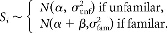The term for motif type and Equation 3 were dropped because the number of familiar and unfamiliar motif types was insufficient to give good estimates for the effects of learning on both between- and within-type variances. The parameter β is the difference in the neuron's average response to familiar and unfamiliar stimuli, and the parameters σ_fam² and σ_unf² are related to the selectivity within each category of motifs.

Model fitting and inference.

Each neuron was fit to the GLMM using JAGS (http://www-fis.iarc.fr/∼martyn/software/jags; version 3.1), a Bayesian modeling toolkit that allows specification of GLMMs and other complex models using a simple equation-like syntax. JAGS uses a Markov Chain Monte Carlo (MCMC) algorithm to sample from the posterior distribution of the model parameters, which are the values of the parameters most likely to give rise to the data.

Bayesian analysis requires prior distributions, which are essentially statements about what values of the parameters are reasonable and likely. The prior for μ, the average spontaneous rate, was N(0, 6.0), a broad distribution with 95% of its density between ∼0.01 and 100 Hz. This range extends well beyond the maximum observed spontaneous rate (25 Hz) in these recordings, while at the lower end the prior serves to regularize the model for the small number of neurons (n = 5) that fired no spikes during baseline recordings. When additional data were available (from recordings of the neuron not used in this analysis), the prior was further refined by setting the prior mean to the empirical spontaneous rate in these recordings, and reducing the prior variance to 1.0 to reflect a higher degree of confidence about the value of μ̄. The prior for α was set to N(1.0, 2.0), corresponding to a belief that for 95% of the neurons the average evoked response would be between ∼0.2 and 40 times the spontaneous rate. When β was included in the model, its prior was N(0.0, 4.0). Noninformative inverse gamma priors were used for the variance parameters.

Posterior distributions were sampled with three independent MCMC chains starting from different initial guesses. After a burn-in period of 25,000 iterations, 30,000 iterations were calculated, keeping every 100th sample. Convergence and stationarity for the parameters of interest were assessed visually and using the Gelman-Rubin diagnostic with R < 1.2 (Brooks and Gelman, 1998). We also generated posterior predictive distributions (samples of the responses we would expect given the data and the model) and compared them to the actual data to visually assess the quality of the fit.

Neurons were considered auditory if there was at least one motif with response strength greater or less than zero (at 95% confidence). Out of a total of 410 well-isolated single units recorded in the target areas, 373 (91%) met this criterion. An additional 21 auditory units were recorded, but could not be unambiguously assigned to one of the target areas and were excluded. Overall selectivity and tolerance were calculated on a sample-by-sample basis from the posterior distributions. It would be possible to add an additional level to the model to compare the distributions of selectivity at the population level, asking, for example, whether different neurons responded to different motifs. Given the great increase in computational complexity such an analysis would imply and lacking strong reasons to assume anything about these distributions, we used point estimates (medians) of the parameters for each neuron. To compare values among areas and spike types, two-way ANOVAs were used followed by post hoc Tukey's tests. Dependent measures were log-transformed or rank-transformed as necessary to achieve normality (assessed by Shapiro–Wilk tests with α = 0.05). When p values for pairwise comparisons are reported in sets, only the largest value is given. To infer the effects of training, we used planned, orthogonal comparisons within each area, i.e., a linear regression of β or σ_fam − σ_unf versus area. The same results obtained using independent t tests in each area, but the linear regression allowed us to test if training affected wide- or narrow-spiking neurons differently, by adding spike type (and its interaction with area) to the regression and evaluating whether the fit improved using ANOVA.

Results

Fourteen adult European starlings of both sexes were trained to recognize two sets of conspecific songs in an operant discrimination task (Gentner and Margoliash, 2003). All the birds achieved accuracies significantly better than chance within 3–11 blocks (mean ± SD = 6.5 ± 2.4; 100 trials per block), 1.0–4.8 d after the start of training (mean ± SD = 2.2 ± 1.1). Birds completed trials at an average rate of 470 ± 110 trials/d (mean ± SD, n = 14). Discrimination performance reached asymptotic levels around block 20 (Fig. 2), with a final d′ of 2.88 ± 0.70 (mean ± SD, n = 14).

Figure 2.

Behavioral performance of starlings during operant discrimination training. Symbols show mean d′ with 95% confidence intervals across birds (n = 14), estimated by bootstrapping. Blocks are 100 trials each.

After training, the responses of 373 auditory single units (7–63 per bird; mean ± SD = 26.6 ± 17.4) were recorded under urethane anesthesia in CLM (n = 75 units from four birds), CMM (63, 6), NCM (49, 5), and subdivisions L1 (39, 4), L2b (39, 7), and L3 (108, 4) of field L. Recorded spikes had either a broad peak and a broad, shallow trough (wide spikes, n = 275), or a narrower peak and a narrow, deep trough (narrow spikes, n = 98). Both classes of neurons were found in all areas, but narrow spikes were more frequently recorded in L1 (n = 16 units, 41%) and L2a (21, 54%) than in CLM (10, 13%), CMM (12, 19%), NCM (14, 29%), or L3 (25, 25%). The nonuniform distribution of narrow and wide spikes across regions was statistically significant (χ² = 29, df = 5, p = 0.0001).

Representative examples of the response patterns evoked by conspecific song stimuli are shown in Figure 3. In all areas, responses were generally characterized by phasic excitatory and suppressive episodes associated with specific acoustic features of the songs. For example, the L2b neuron responded strongly coincident with a low-frequency broadband element present in several motifs and both songs (Fig. 3b), while the L3 neuron responded strongly at the ends of only four of the motifs (Fig. 3c). These responses may reflect tuning to simple low-level acoustic features, as seen earlier in the auditory pathway (Woolley et al., 2009), tuning to more complex vocal elements, as previously reported for CMM neurons (Meliza et al., 2010), or some combination of these properties. Until further testing, such hypotheses are speculative, but from these data one can objectively ascertain that the L3 neuron was more selective, in the sense that it responded only during a small proportion of the presented stimuli. In contrast, the L2b neuron was active almost throughout all stimuli.

Figure 3.

Responses of exemplar neurons. a, Spectrograms (top) show two of the song stimuli presented to the six neurons below, each a representative from one of the six auditory areas. Responses are shown as raster plots, with vertical ticks indicating the spike times and each row corresponding to the response on a different trial. Vertical gray lines mark the onsets of the component motifs. Traces on the far right show the average shape of each neuron's spikes. The CMM and L2b spikes were classified as narrow; the others were wide (see Materials and Methods). b, Detail of motifs 4–5 and 9–10 in the first and second songs, respectively, with histogram of the L2b neuron's response below (bin size = 20 ms). c, Detail of motifs 1–4 in the second song, with histogram of the L3 neuron's response. Detail spectrograms have same frequency scale as in a.

Motif selectivity differs between areas

To quantify selectivity, the responses were divided into intervals corresponding to motifs (Fig. 3a, vertical gray lines), and the average firing rate during each interval was taken as the response strength for the corresponding motif. The distribution of response strength over the set of presented motifs gives a measure of its selectivity. Selective neurons responded strongly to a few motifs and weakly to the rest, resulting in narrow distributions with long tails (for example, Fig. 4a, L3, cyan trace). Nonselective neurons responded similarly to all the motifs, resulting in broad response distributions (Fig. 4a, L2b, cyan trace). Comparing these distributions between areas, there were clear qualitative differences. All the areas exhibited a fairly broad range of selectivity, but L1 and L2b had few of the highly selective units seen in the other areas. CLM and CMM had the broadest range of selectivities, and in NCM and L3 the distribution appeared to be skewed toward more selective neurons. When the neurons in each area were separated into groups based on spike shape (Fig. 4b,c), the wide-spike neurons appeared to be more selective on average (Fig. 4a, compare blue and red lines).

To quantify differences in the shapes of response strength distributions, we first used the AF or sparseness index (Vinje and Gallant, 2000; Lehky et al., 2005; see Materials and Methods). This index is 0 if a neuron responds the same to all stimuli, and 1 if it responds to only one. There were significant differences in selectivity among areas (Fig. 4d; two-way rank-transformed ANOVA: F_(5,361) = 14.28, p = 10⁻¹⁴). Selectivity in L3 and NCM was greater than in the other areas (Tukey's tests: p ≤ 0.01), but not significantly different between L3 and NCM or between any of the other areas. This result was unexpected, given that L3 is often considered to be at a similar level of the auditory hierarchy as L1. Across areas, wide-spiking neurons were more selective than narrow-spiking neurons (F_(1,361) = 6.66, p = 0.01), and there was no significant interaction between area and spike type (F_(5,361) = 0.23, p = 0.95).

Selectivity between and within motif types differs among areas

A concern in using AF to quantify selectivity is that the stimuli are not equally different from each other. Starling songs often contain repeated renditions of the same motif type that vary slightly in pitch, duration, and note complement (Figs. 3b,c, 5a). Some neurons were more tolerant of this within-type variability than others. For example, the CMM neuron in Figure 5a gave similar responses to each variant of motif types A and B, whereas the NCM neuron responded more strongly to the first instance of A and most strongly to the last instance of B. This difference can be clearly observed in plots of the response distribution where motifs are grouped by type. For the CMM neuron (Fig. 5b) the within-type variance was low, indicated by points closely scattered about the means for each type. In contrast, the NCM neuron (Fig. 5c) had a high within-type variance, indicated by the large scatter about the means for each type.

Figure 5.

Variability within motif types and neuronal tolerance. a, Spectrogram of a song segment comprising two distinct motif types (A, B) repeated with variations in acoustic structure. Below are rasters of responses from a CMM and an NCM neuron demonstrating tolerance (CMM) and sensitivity (NCM) to motif variability. b, Mean response of the CMM neuron to each of the presented motif variants (gray circles), grouped by type. Hollow squares indicate the average for each type, and the x-axis is in ascending order of these averages. A and B labels correspond to the motif types shown in a. Horizontal gray line indicates spontaneous firing rate. c, The motif type and variant distribution for the exemplar NCM neuron, illustrating the greater variance in its responses to motif variants. Both neurons were presented with the same set of motifs.

To quantify the between- and within-type variances, we developed a GLMM. This model partitions the variance in the responses of single units into two stimulus-dependent terms, the motif type and variant, and two stimulus-independent terms associated with the spontaneous rate and other stochastic factors (see Materials and Methods). For the example CMM neuron (Fig. 5b), the model indicated a between-type variance of 0.45 and a within-type variance of 0.02; for the NCM neuron (Fig. 5c), the between-type variance was 0.24 and the within-type variance was 1.04.

As a test of the model, we first looked at the overall selectivity of the neurons by pooling the between- and within-type variances and normalizing by the stimulus-independent variance (S′; see Materials and Methods). Similar to the results obtained using AF, S′ indicated significant increases in selectivity from L1 and L2b to L3 and NCM (Fig. 6a). The two metrics were highly correlated (r = 0.80; t₍₃₇₁₎ = 25.3, p < 10⁻¹⁵) and their distributions in each area were similar (compare Figs. 4d, 6a). One notable exception was for the wide-spike neurons in L3. Whereas AF for these neurons was uniformly distributed across the range of the metric, S′ was skewed such that a large proportion of the neurons had selectivity less than the mean. Other areas did not show this degree of compression. We hypothesize that this difference reflects the way the two metrics handle stimulus-independent variability. AF uses point estimates of the response strength for each stimulus. Increased intertrial variability results in increased variance of these estimates, and thus AF can be positively biased by noise (Rust and DiCarlo, 2012). In contrast, the GLMM explicitly includes terms for stimulus-independent variability, which are factored out to provide unbiased estimates of stimulus-dependent variability. Consistent with this hypothesis, wide-spiking neurons had higher stimulus-independent variability than narrow-spiking neurons, particularly in L3 (Fig. 6b). The functional significance of greater intertrial variability in some areas and classes of neurons is unclear, but may reflect more nonlinear integration or increased input from nonauditory areas.

Figure 6.

Selectivity and stimulus-independent variance of neural responses in different regions of the auditory cortex. a, Overall selectivity (S′; see Materials and Methods) of neurons by area and spike type (red symbols, narrow spikes; blue symbols, wide spikes). There are significant differences among areas (two-way log-transformed ANOVA: F_(5,361) = 12.27, p = 10⁻¹⁰), but not between spike types (F_(1,361) = 0.50, p = 0.48) or for their interaction (F_(5,361) = 1.61, p = 0.16). b, Stimulus-independent variability. Differences among areas and between spike types are significant (two-way rank-transformed ANOVA: F_(5,361) = 9.26, p = 10⁻⁷; F_(1,361) = 27.40, p = 10⁻⁶), but the interaction is not (F_(5,361) = 1.89, p = 0.10). In a and b, circles are individual neurons (horizontally jittered for clarity). Error bars indicate mean ± SE. Areas are ordered as in Figure 4d. *, Significant post hoc differences between areas, with p < 0.05.

When examined separately, between- and within-type selectivity had the same generally increasing trend as seen for overall selectivity. However, the relative contributions of these terms differed among areas. Between-type selectivity was lower in L1 and L2b and higher in CMM, NCM, and L3 (Fig. 7a). There also appeared to be a large number of wide-spiking neurons in CLM that had high between-type selectivity, but as there was no significant interaction between area and spike type, no statistical inferences about this difference could be made. In contrast, within-type selectivity was low in L1, L2b, CLM, and CMM, and high in NCM and L3 (Fig. 7b), indicating that neurons in CLM and CMM were sensitive to the differences among types and tolerant of the differences among variants, whereas NCM and L3 neurons were sensitive to differences both among and within types. This increased selectivity between variants of the same type might indicate a sensitivity to small-scale acoustic differences as well as sensitivity to larger scale differences in the sequence and context of the motifs.

Figure 7.

Tolerance for within-type variability differs among areas. a, Selectivity between motif types by area and spike type (red symbols, narrow spikes; blue symbols, wide spikes). Differences among areas are significant (two-way rank-transformed ANOVA: F_(5,361) = 8.24, p = 10⁻⁶), but not between spike types (F_(1,361) = 1.56, p = 0.21) or for the interaction (F_(5,361) = 0.78, p = 0.57). b, Selectivity between variants of the same motif type. Differences among areas are significant (two-way rank-transformed ANOVA: F_(5,361) = 11.64, p = 10⁻⁹; Tukey's tests: p ≤ 0.04), but not the effect of spike type (F_(1,361) = 0.15, p = 0.70) or the interaction (F_(1,361) = 1.31, p = 0.26). c, Tolerance, defined as the ratio of between-type variance to the total stimulus-dependent variance. Differences among areas and between spike types are significant (two-way rank-transformed ANOVA: F_(5,361) = 5.98, p = 0.0003; F_(1,361) = 3.89, p = 0.049), but the interaction is not (F_(5,361) = 0.91, p = 0.48). In a–c, circles are individual neurons (horizontally jittered for clarity). Error bars indicate mean ± SE. Areas are ordered as in Figure 4d. *, Significant post hoc differences between areas, with p < 0.05.

To test whether individual neurons were more sensitive to between- or within-type differences, we calculated a tolerance index, defined as the ratio of between-type variance to the total stimulus-dependent variance: T = σ_type²/(σ_type² + σ_variant²). For a perfectly tolerant neuron that responded identically to every variant of all the motif types, the between-type variance would be equal to the total variance, giving T = 1. As within-type variance increases, T approaches zero. For the exemplar CMM and NCM neurons (Fig. 5), T was 0.96 and 0.18, respectively. As seen in Figure 7c, CLM and CMM were both highly tolerant relative to other areas, and wide-spike neurons were more tolerant (mean ± SE = 0.51 ± 0.02) than narrow-spike neurons (0.40 ± 0.03; F_(1,361) = 3.89, p = 0.049). In L3, the tolerance did not differ significantly from any of the other areas, but among wide-spike neurons the distribution appeared to be multimodal, with large clusters of neurons tending to have low, medium, or high tolerance.

NCM is considered to be secondary auditory cortex, yet it exhibited particularly low tolerance (Fig. 7c). One possibility is that differences in its responses to the same motif types might in fact reflect sensitivity for sequence or context, in which case neurons might respond preferentially to the first or last variant in a run (Fig. 5a). As a post hoc test of this hypothesis, we used a simple mixed-effects model to determine whether the first or last variants in runs of the same type were stronger or weaker than motifs from the middle. The effect was not significant (p = 0.89), indicating that there was no consistent primacy or recency effect in NCM. However, a stronger test, in which the order of variants is manipulated, is necessary to determine whether NCM is sensitive to more global contextual features.

Spontaneous firing rates were lower in L3 than any other area (two-way ANOVA: F_(5,361) = 12.33, p = 10⁻¹⁰; Tukey's tests: p ≤ 0.002), and lower for wide-spiking neurons (F_1,361 = 5.44, p = 0.02), but there was no significant interaction between spike type and area. Across areas and spike types, there was a negative correlation between spontaneous rate and selectivity (r = –0.6, t₍₃₇₁₎ = −14, p = 10⁻¹⁵); when the data were split into separate areas the correlation was significant in all areas except L1. Across areas, there was no significant correlation between tolerance (T) and selectivity (S′; r = 0.02, p = 0.66), but when the data were split by area the correlation within CMM was significantly negative (r = –0.32, p = 0.01).

Learning affects selectivity and average response strength in CMM and NCM

Out of the 373 auditory units, 323 (87%) remained isolated long enough to record sufficient responses to both familiar and unfamiliar stimuli (n = 73, 55, 41, 31, 28, 95 units in areas CLM, CMM, NCM, L1, L2b, and L3). For many neurons, there were striking differences in the distribution of responses to the two categories. Some neurons were more selective within one category of stimuli than the other. For example, the CMM neuron shown in Figure 8a had nearly the same average response to familiar motifs (open circles) as to unfamiliar motifs (filled squares), but the variance was much higher among the familiar motifs (compare error bars). Other neurons, like the NCM neuron in Figure 8b, were more similar in their selectivity within each category, but showed a difference in the means (i.e., a bias for one category over the other).

Figure 8.

Effects of training on response distributions. a, Response strength distribution of exemplar CMM neuron (from Fig. 3) with motifs coded for familiarity (open circles) and unfamiliarity (filled squares). Larger symbols indicate mean ± SD for each category. Horizontal gray line, average spontaneous rate. b, The same plot for the exemplar NCM neuron. c, Bias, the difference in mean response to familiar and unfamiliar motifs, by area. Circles represent individual neurons. Horizontal bars, mean for each area with 95% confidence intervals. *p < 0.05. d, SD between familiar motifs is plotted against SD between unfamiliar motifs for each area. The diagonal line indicates equality. Circles are individual neurons; squares indicate the mean difference with 95% confidence intervals. **p < 0.01. Both axes are on a log scale for visual clarity. No significant effect of spike type was observed on bias or the difference in selectivity, so the two classes of neurons are pooled in this figure.

To quantify these effects, we modified the GLMM to include an independent mean and variance term for each category of motifs. We also removed the term associated with motif types, as the number of unique motif types in each category was not large enough to give reliable estimates for all the parameters. Using this model for the exemplar CMM neuron (Fig. 8a), the difference in means (bias) was –0.06 log Hz and the difference in selectivity (S′) was 0.39. In contrast, the NCM neuron (Fig. 8b) had a bias of –0.14 log Hz and a selectivity difference of –0.23, indicating that both the mean and variance were lower for familiar motifs.

In NCM, the average bias was significantly less than zero (mean ± SE = –0.23 ± 0.10 log Hz; planned contrast: p = 0.029; Fig. 8c), indicating that response strengths were 20% lower on average for familiar motifs. There was a tendency in all areas for the magnitude of the bias to increase with selectivity because of sampling variability (for the neurons that responded to few motifs, the probability that those motifs would be evenly balanced between familiar and unfamiliar was low even if the true bias was zero). However, the average bias was not significantly different from zero in any other area but NCM. The effect of spike type was not significant (ANOVA: F_(6,311) = 1.52; p = 0.17).

CMM neurons, on the other hand, were consistently more selective between familiar motifs than between unfamiliar motifs (Fig. 8d). As with bias, many individual neurons in all areas showed large differences in within-category selectivity by chance. Only in CMM was there a significant difference in the population (mean difference ± SE = 0.21 ± 0.08; planned contrast: p = 0.005). As with bias, there was no significant difference in the effect of training on wide- and narrow-spiking neurons (ANOVA: F_(6,311) = 0.84; p = 0.54). The increase in selectivity due to familiarity, without a concomitant increase in average response strength, suggests that learning led to increased excitation for some motifs and increased suppression for others, as in Figure 8a.

Discussion

These results demonstrate differences in selectivity and tolerance between areas of the starling auditory cortex. Areas L1 and L2b exhibited low selectivity, responding similarly across a broad range of stimuli. L3 and NCM were distinctly more selective than other areas. CLM and CMM exhibited intermediate levels of selectivity, but they were more tolerant than other areas of differences between renditions of the same motif types. The effects of perceptual song learning were evident principally in CMM and NCM. Our results support a functional hierarchical view of the avian auditory cortex but motivate a revision of that view, and indicate a divergence within the cortical hierarchy into parallel, functionally distinct streams.

Selectivity and tolerance in the avian auditory system

In songbirds, conspecific songs elicit responses from neurons throughout the auditory cortex, including higher order areas where many neurons respond selectively to a subset of songs (Leppelsack and Vogt, 1976; Müller and Leppelsack, 1985; Chew et al., 1996). One method of assessing selectivity is through receptive field (RF) models, which represent neuronal responses as functions of low-level acoustic properties of the stimulus. Models based on the spectrotemporal envelope (Theunissen et al., 2001) have provided significant insight into processing in the midbrain, thalamus, and primary thalamorecipient cortex (Woolley et al., 2009), but at higher levels RFs become more nonlinear and more difficult to model (Sen et al., 2001; Sharpee et al., 2011). Here, rather than attempt to characterize RFs, we took a complementary approach of characterizing the distributions of neuronal responses over a broad range of representative stimuli. These distributions reflect the relationship between the neuron's RF and the distribution of features in the stimuli.

We assessed response selectivity using a statistical framework to evaluate the sources of variation in the neuronal responses. We hypothesized that neurons would differ in sensitivity to variability between motif types and variability within motif types, and that neurons would differ across areas in the amount of information they carried about motif types. The novel mixed-effects model-based approach we developed allowed us to measure the variance in the neuronal responses to different motif types along with the variance due to other stimulus-dependent and -independent factors.

This model yielded similar measures of overall selectivity as AF (or sparseness; Vinje and Gallant, 2000), a commonly used nonparametric selectivity index. In its approach to factoring out stimulus-independent variance, it is similar in principle to mutual information (Rolls et al., 1997; Nelken and Chechik, 2007), but where mutual information quantifies the amount of response entropy that depends on stimulus identity, the mixed-effects model uses only the variance. The advantages of the model-based approach are that the variance estimates are robust and almost completely unbiased (see Materials and Methods) and can be flexibly partitioned to reflect structure in the task or stimuli.

The results indicate three groupings of starling auditory areas. L1 and L2b had low selectivity within and among motif types, indicating that they responded to features common to many stimuli. CMM and a subpopulation of wide-spiking neurons in CLM exhibited increased selectivity among types, suggesting that they were more sensitive to features that differed among types. NCM and L3 were more selective among types than L1 or L2b, but were also more selective among variants of the same types. This sensitivity, or lack of tolerance, could be to local differences in the pitch, duration, or complement of notes in the variants, to the song context in which the variant occurs, or to both.

We note that these data are from urethane-anesthetized birds, which facilitated collecting relatively large samples in single experiments from each bird. In earlier CMM recordings (Meliza et al., 2010), we found that urethane reduced spike precision and intertrial correlation but did not significantly affect selectivity. In the midbrain, urethane reduces intrinsic excitability but does not affect selectivity (Schumacher et al., 2011), and studies in field L have also found no effect on selectivity (Narayan et al., 2006). We expect that some measures of selectivity may be higher in awake birds as a result of decreased stimulus-independent variability, but that relative differences between areas are likely to remain unchanged.

Effects of learning on response distributions

Motifs were also grouped into categories based on whether the animal had learned them in an operant task. Familiar motifs were behaviorally salient, associated with specific responses and reward contingencies, whereas unfamiliar motifs had no such associations. In NCM, responses were significantly weaker to familiar motifs (Thompson and Gentner, 2010). In CMM, the selectivity among familiar motifs was higher than for unfamiliar motifs (Gentner and Margoliash, 2003; Jeanne et al., 2011). This effect is likely to reflect increased selectivity between stimuli associated with different behavioral responses (i.e., left vs right, or S+ vs S−) as well as increased selectivity within each of these categories (Jeanne et al., 2011). Additional experiments are necessary to determine whether training affects within-type and within-category tolerance in a manner that would support the emergence of learned categorical perception (Sigala and Logothetis, 2002).

Divergent hierarchical processing in support of natural category recognition

Our results fit into a hierarchical view of the physiological organization of the avian cortex but modify the prevailing conception of that hierarchy. Taken together, anatomical and physiological studies have been interpreted to support a feedforward hierarchy with L2a at the lowest level; L2b, L1, and L3 at intermediate levels; and CLM, CMM, and NCM at the highest (Theunissen and Shaevitz, 2006). The present results are consistent with some aspects of this model. The secondary areas NCM, CLM, and CMM are more selective among types and/or variants than L1 and L2b, and both NCM and CMM exhibited the expected learning-dependent effects. Strikingly, however, L3 was much more selective than L1, L2b, and even CLM. Previous studies of field L did not report differences between L1 and L3 in starlings (Bonke et al., 1979; Scheich et al., 1979; Müller and Leppelsack, 1985) or zebra finches (Sen et al., 2001; Nagel and Doupe, 2008), and many studies pool results from all of field L (excluding L2a). The spectrotemporal RF models used in more recent studies, however, predict <25% of the variance of responses outside L2a and may have failed to capture critical nonlinearities that contribute to differences in selectivity. Additionally, the most selective neurons in L3 have extremely low spontaneous rates (Scheich et al., 1979) and were typically only detected on other channels of the electrode after recording was started. Single channel electrodes may introduce greater biases against sampling such neurons.

The differences in selectivity and tolerance seen in this study can be related to recent insights into the connectivity within the avian auditory cortex. In chicks, projections within field L and CM are radially organized and span both areas (Wang et al., 2010). The pattern of connections between subdivisions is similar to the canonical interlaminar circuit in mammalian auditory cortex (A1), from thalamorecipient L2a to superficial L1 and CLM and then deeper to L3 (Fig. 9). The broad range of selectivity in CLM including possible differences between narrow- and wide-spiking neurons (which are thought to correspond to inhibitory interneurons and excitatory projection neurons (McCormick et al., 1985; Atencio and Schreiner, 2008), suggest that local processing may result in increased selectivity among motif types. Local connectivity is high within CLM (Vates et al., 1996), as it is in layer 2/3 of neocortex (Douglas and Martin, 2004). High selectivity in L3 is consistent with its position as an output of the avian auditory cortex. L3 selectivity may be inherited from CLM and passed on to NCM and descending pathways.

Figure 9.

Cortical model of avian auditory processing. Canonical interlaminar connectivity of primary mammalian auditory cortex. Connectivity among subdivisions of field L, CM, and NCM. The primary (lateral) areas show a similar pattern of connectivity from thalamorecipient to superficial to deep layers. There are separate connections from superficial and deep areas of the field L/CLM complex to the putative secondary areas CMM and NCM. Adapted from Wang et al. (2010) with addition of L2b, CMM, and NCM. The blue line represents thalamic input, the red circles and arrows indicate intrinsic connections, and the cyan arrow indicates descending projections. For clarity, the projection from L2b to NCM has been omitted, as well as connections from the shell of ovoidalis to L1, L3, and NCM, which are more diffuse and not tonotopic.

Both NCM and CMM showed effects of learning in their responses, a hallmark of secondary sensory areas (Kobatake et al., 1998; Freedman et al., 2006). In this view, connections between CLM and CMM, and between L3 and NCM might represent corticocortical connections to secondary or auxiliary auditory cortex (Fig. 9). Interestingly, the two mesopallial areas exhibited high selectivity and high tolerance, whereas L3 and NCM in the nidopallium were characterized by high selectivity and low tolerance. We propose that auditory processing diverges within CLM into functionally specialized nidopallial and mesopallial pathways culminating in CMM and NCM. In NCM, neurons were sensitive to differences within motif types and responded more to novel stimuli, suggesting that it may act as a novelty detector. In contrast, learning increased selectivity in CMM. Learning may play a role in the acquisition of tolerance in the mesopallium, if the learned features are ones that vary between different motif types. CMM may form invariant representations of motif types that can be associated with specific behavioral categories.

The proposed processing hierarchy shares several features with the mammalian auditory cortex (Fig. 9) (Atencio et al., 2009). The pattern of connections is consistent with recent molecular evidence homologizing regions of avian forebrain with neocortex (Dugas-Ford et al., 2012). We propose that object and category recognition rely on circuit mechanisms that are conserved across modalities and phylogenetic taxa.

References

- Adret-Hausberger M, Jenkins P. Complex organization of the warbling song in starlings. Behaviour. 1988;107:138–156. [Google Scholar]
- Atencio CA, Schreiner CE. Spectrotemporal processing differences between auditory cortical fast-spiking and regular-spiking neurons. J Neurosci. 2008;28:3897–3910. doi: 10.1523/JNEUROSCI.5366-07.2008. [DOI] [PMC free article] [PubMed] [Google Scholar]
- Atencio CA, Sharpee TO, Schreiner CE. Hierarchical computation in the canonical auditory cortical circuit. Proc Natl Acad Sci U S A. 2009;106:21894–21899. doi: 10.1073/pnas.0908383106. [DOI] [PMC free article] [PubMed] [Google Scholar]
- Bonke D, Scheich H, Langner G. Responsiveness of units in the auditory neostriatum of the guinea fowl (Numida meleagris) to species-specific calls and synthetic stimuli. I. Tonotopy and functional zones. J Comp Physiol. 1979;132:243–255. [Google Scholar]
- Brooks SP, Gelman A. General methods for monitoring convergence of iterative simulations. J Comput Graph Stat. 1998;7:434–455. [Google Scholar]
- Chew SJ, Vicario DS, Nottebohm F. A large-capacity memory system that recognizes the calls and songs of individual birds. Proc Natl Acad Sci U S A. 1996;93:1950–1955. doi: 10.1073/pnas.93.5.1950. [DOI] [PMC free article] [PubMed] [Google Scholar]
- David SV, Hayden BY, Gallant JL. Spectral receptive field properties explain shape selectivity in area V4. J Neurophysiol. 2006;96:3492–3505. doi: 10.1152/jn.00575.2006. [DOI] [PubMed] [Google Scholar]
- Desimone R, Albright TD, Gross CG, Bruce C. Stimulus-selective properties of inferior temporal neurons in the macaque. J Neurosci. 1984;4:2051–2062. doi: 10.1523/JNEUROSCI.04-08-02051.1984. [DOI] [PMC free article] [PubMed] [Google Scholar]
- Douglas RJ, Martin KA. Neuronal circuits of the neocortex. Annu Rev Neurosci. 2004;27:419–451. doi: 10.1146/annurev.neuro.27.070203.144152. [DOI] [PubMed] [Google Scholar]
- Dugas-Ford J, Rowell JJ, Ragsdale CW. Cell type homologies and the origins of the neocortex. Proc Natl Acad Sci U S A. 2012 doi: 10.1073/pnas.1204773109. in press. [DOI] [PMC free article] [PubMed] [Google Scholar]
- Eens M, Pinxten R, Verheyen RF. Temporal and sequential organization of song bouts in the European starling. Ardea. 1989;77:75–86. [Google Scholar]
- Escabí MA, Read HL. Representation of spectrotemporal sound information in the ascending auditory pathway. Biol Cybern. 2003;89:350–362. doi: 10.1007/s00422-003-0440-8. [DOI] [PubMed] [Google Scholar]
- Falls JB. Individual recognition by sound in birds. In: Kroodsma DE, Miller EH, editors. Acoustic communication in birds. New York: Academic; 1982. pp. 237–278. [Google Scholar]
- Fortune ES, Margoliash D. Cytoarchitectonic organization and morphology of cells of the field L complex in male zebra finches (Taenopygia guttata) J Comp Neurol. 1992;325:388–404. doi: 10.1002/cne.903250306. [DOI] [PubMed] [Google Scholar]
- Freedman DJ, Assad JA. Experience-dependent representation of visual categories in parietal cortex. Nature. 2006;443:85–88. doi: 10.1038/nature05078. [DOI] [PubMed] [Google Scholar]
- Freedman DJ, Riesenhuber M, Poggio T, Miller EK. Experience-dependent sharpening of visual shape selectivity in inferior temporal cortex. Cereb Cortex. 2006;16:1631–1644. doi: 10.1093/cercor/bhj100. [DOI] [PubMed] [Google Scholar]
- Frey BJ, Dueck D. Clustering by passing messages between data points. Science. 2007;315:972–976. doi: 10.1126/science.1136800. [DOI] [PubMed] [Google Scholar]
- Gelman A, Hill J. Data analysis using regression and multilevel/hierarchical models. Cambridge, UK: Cambridge UP; 2006. [Google Scholar]
- Gentner TQ. Neural systems for individual song recognition in adult birds. Ann N Y Acad Sci. 2004;1016:282–302. doi: 10.1196/annals.1298.008. [DOI] [PubMed] [Google Scholar]
- Gentner TQ, Hulse SH. Perceptual mechanisms for individual vocal recognition in European starlings, Sturnus vulgaris. Anim Behav. 1998;56:579–594. doi: 10.1006/anbe.1998.0810. [DOI] [PubMed] [Google Scholar]
- Gentner TQ, Margoliash D. Neuronal populations and single cells representing learned auditory objects. Nature. 2003;424:669–674. doi: 10.1038/nature01731. [DOI] [PMC free article] [PubMed] [Google Scholar]
- Hazan L, Zugaro M, Buzsáki G. Klusters, NeuroScope, NDManager: a free software suite for neurophysiological data processing and visualization. J Neurosci Methods. 2006;155:207–216. doi: 10.1016/j.jneumeth.2006.01.017. [DOI] [PubMed] [Google Scholar]
- Hillenbrand J, Getty LA, Clark MJ, Wheeler K. Acoustic characteristics of American English vowels. J Acoust Soc Am. 1995;97:3099–3111. doi: 10.1121/1.411872. [DOI] [PubMed] [Google Scholar]
- Hsu A, Woolley SM, Fremouw TE, Theunissen FE. Modulation power and phase spectrum of natural sounds enhance neural encoding performed by single auditory neurons. J Neurosci. 2004;24:9201–9211. doi: 10.1523/JNEUROSCI.2449-04.2004. [DOI] [PMC free article] [PubMed] [Google Scholar]
- Hubel DH, Wiesel TN. Receptive fields and functional architecture in two nonstriate visual areas (18 and 19) of the cat. J Neurophysiol. 1965;28:229–289. doi: 10.1152/jn.1965.28.2.229. [DOI] [PubMed] [Google Scholar]
- Jeanne JM, Thompson JV, Sharpee TO, Gentner TQ. Emergence of learned categorical representations within an auditory forebrain circuit. J Neurosci. 2011;31:2595–2606. doi: 10.1523/JNEUROSCI.3930-10.2011. [DOI] [PMC free article] [PubMed] [Google Scholar]
- Karten HJ. The ascending auditory pathway in the pigeon (Columba livia). II. Telencephalic projections of the nucleus ovoidalis thalami. Brain Res. 1968;11:134–153. doi: 10.1016/0006-8993(68)90078-4. [DOI] [PubMed] [Google Scholar]
- Kobatake E, Tanaka K. Neuronal selectivities to complex object features in the ventral visual pathway of the macaque cerebral cortex. J Neurophysiol. 1994;71:856–867. doi: 10.1152/jn.1994.71.3.856. [DOI] [PubMed] [Google Scholar]
- Kobatake E, Wang G, Tanaka K. Effects of shape-discrimination training on the selectivity of inferotemporal cells in adult monkeys. J Neurophysiol. 1998;80:324–330. doi: 10.1152/jn.1998.80.1.324. [DOI] [PubMed] [Google Scholar]
- Lehky SR, Sejnowski TJ, Desimone R. Selectivity and sparseness in the responses of striate complex cells. Vision Res. 2005;45:57–73. doi: 10.1016/j.visres.2004.07.021. [DOI] [PMC free article] [PubMed] [Google Scholar]
- Leppelsack HJ, Vogt M. Responses of auditory neurons in the forebrain of a songbird to stimulation with species-specific sounds. J Comp Physiol. 1976;107:263–274. [Google Scholar]
- Logothetis NK, Pauls J, Poggio T. Shape representation in the inferior temporal cortex of monkeys. Curr Biol. 1995;5:552–563. doi: 10.1016/s0960-9822(95)00108-4. [DOI] [PubMed] [Google Scholar]
- Macmillan NA, Kaplan HL, Creelman CD. The psychophysics of categorical perception. Psychol Rev. 1977;84:452–471. [PubMed] [Google Scholar]
- Margoliash D. Preference for autogenous song by auditory neurons in a song system nucleus of the white-crowned sparrow. J Neurosci. 1986;6:1643–1661. doi: 10.1523/JNEUROSCI.06-06-01643.1986. [DOI] [PMC free article] [PubMed] [Google Scholar]
- McCormick DA, Connors BW, Lighthall JW, Prince DA. Comparative electrophysiology of pyramidal and sparsely spiny stellate neurons of the neocortex. J Neurophysiol. 1985;54:782–806. doi: 10.1152/jn.1985.54.4.782. [DOI] [PubMed] [Google Scholar]
- Meliza CD, Chi Z, Margoliash D. Representations of conspecific song by starling secondary forebrain auditory neurons: towards a hierarchical framework. J Neurophysiol. 2010;103:1195–1208. doi: 10.1152/jn.00464.2009. [DOI] [PMC free article] [PubMed] [Google Scholar]
- Müller CM, Leppelsack HJ. Feature extraction and tonotopic organization in the avian auditory forebrain. Exp Brain Res. 1985;59:587–599. doi: 10.1007/BF00261351. [DOI] [PubMed] [Google Scholar]
- Nagel KI, Doupe AJ. Organizing principles of spectro-temporal encoding in the avian primary auditory area field L. Neuron. 2008;58:938–955. doi: 10.1016/j.neuron.2008.04.028. [DOI] [PMC free article] [PubMed] [Google Scholar]
- Narayan R, Graña G, Sen K. Distinct time scales in cortical discrimination of natural sounds in songbirds. J Neurophysiol. 2006;96:252–258. doi: 10.1152/jn.01257.2005. [DOI] [PubMed] [Google Scholar]
- Nelken I, Chechik G. Information theory in auditory research. Hear Res. 2007;229:94–105. doi: 10.1016/j.heares.2007.01.012. [DOI] [PubMed] [Google Scholar]
- Reiner A, et al. Revised nomenclature for avian telencephalon and some related brainstem nuclei. J Comp Neurol. 2004;473:377–414. doi: 10.1002/cne.20118. [DOI] [PMC free article] [PubMed] [Google Scholar]
- Riesenhuber M, Poggio T. Neural mechanisms of object recognition. Curr Opin Neurobiol. 2002;12:162–168. doi: 10.1016/s0959-4388(02)00304-5. [DOI] [PubMed] [Google Scholar]
- Rolls ET. Functions of the primate temporal lobe cortical visual areas in invariant visual object and face recognition. Neuron. 2000;27:205–218. doi: 10.1016/s0896-6273(00)00030-1. [DOI] [PubMed] [Google Scholar]
- Rolls ET, Treves A, Tovee MJ, Panzeri S. Information in the neuronal representation of individual stimuli in the primate temporal visual cortex. J Comput Neurosci. 1997;4:309–333. doi: 10.1023/a:1008899916425. [DOI] [PubMed] [Google Scholar]
- Rust NC, Dicarlo JJ. Balanced increases in selectivity and tolerance produce constant sparseness along the ventral visual stream. J Neurosci. 2012;32:10170–10182. doi: 10.1523/JNEUROSCI.6125-11.2012. [DOI] [PMC free article] [PubMed] [Google Scholar]
- Scheich H, Langner G, Bonke D. Responsiveness of units in the auditory neostriatum of the Guinea fowl (Numida meleagris) to species-specific calls and synthetic stimuli. II. Discrimination of iambus-like calls. J Comp Physiol. 1979;132:257–276. [Google Scholar]
- Schumacher JW, Schneider DM, Woolley SM. Anesthetic state modulates excitability but not spectral tuning or neural discrimination in single auditory midbrain neurons. J Neurophysiol. 2011;106:500–514. doi: 10.1152/jn.01072.2010. [DOI] [PMC free article] [PubMed] [Google Scholar]
- Sen K, Theunissen FE, Doupe AJ. Feature analysis of natural sounds in the songbird auditory forebrain. J Neurophysiol. 2001;86:1445–1458. doi: 10.1152/jn.2001.86.3.1445. [DOI] [PubMed] [Google Scholar]
- Sharp SP, McGowan A, Wood MJ, Hatchwell BJ. Learned kin recognition cues in a social bird. Nature. 2005;434:1127–1130. doi: 10.1038/nature03522. [DOI] [PubMed] [Google Scholar]
- Sharpee TO, Atencio CA, Schreiner CE. Hierarchical representations in the auditory cortex. Curr Opin Neurobiol. 2011;21:761–767. doi: 10.1016/j.conb.2011.05.027. [DOI] [PMC free article] [PubMed] [Google Scholar]
- Sigala N, Logothetis NK. Visual categorization shapes feature selectivity in the primate temporal cortex. Nature. 2002;415:318–320. doi: 10.1038/415318a. [DOI] [PubMed] [Google Scholar]
- Suga N. Specialization of the auditory system for reception and processing of species-specific sounds. Fed Proc. 1978;37:2342–2354. [PubMed] [Google Scholar]
- Theunissen FE, Shaevitz SS. Auditory processing of vocal sounds in birds. Curr Opin Neurobiol. 2006;16:400–407. doi: 10.1016/j.conb.2006.07.003. [DOI] [PubMed] [Google Scholar]
- Theunissen FE, David SV, Singh NC, Hsu A, Vinje WE, Gallant JL. Estimating spatio-temporal receptive fields of auditory and visual neurons from their responses to natural stimuli. Network. 2001;12:289–316. [PubMed] [Google Scholar]
- Theunissen FE, Woolley SM, Hsu A, Fremouw T. Methods for the analysis of auditory processing in the brain. Ann N Y Acad Sci. 2004;1016:187–207. doi: 10.1196/annals.1298.020. [DOI] [PubMed] [Google Scholar]
- Thompson JV, Gentner TQ. Song recognition learning and stimulus-specific weakening of neural responses in the avian auditory forebrain. J Neurophysiol. 2010;103:1785–1797. doi: 10.1152/jn.00885.2009. [DOI] [PMC free article] [PubMed] [Google Scholar]
- Vates GE, Broome BM, Mello CV, Nottebohm F. Auditory pathways of caudal telencephalon and their relation to the song system of adult male zebra finches. J Comp Neurol. 1996;366:613–642. doi: 10.1002/(SICI)1096-9861(19960318)366:4<613::AID-CNE5>3.0.CO;2-7. [DOI] [PubMed] [Google Scholar]
- Vinje WE, Gallant JL. Sparse coding and decorrelation in primary visual cortex during natural vision. Science. 2000;287:1273–1276. doi: 10.1126/science.287.5456.1273. [DOI] [PubMed] [Google Scholar]
- Wang Y, Brzozowska-Prechtl A, Karten HJ. Laminar and columnar auditory cortex in avian brain. Proc Natl Acad Sci U S A. 2010;107:12676–12681. doi: 10.1073/pnas.1006645107. [DOI] [PMC free article] [PubMed] [Google Scholar]
- Wild JM, Karten HJ, Frost BJ. Connections of the auditory forebrain in the pigeon (Columba livia) J Comp Neurol. 1993;337:32–62. doi: 10.1002/cne.903370103. [DOI] [PubMed] [Google Scholar]
- Woolley SM, Gill PR, Fremouw T, Theunissen FE. Functional groups in the avian auditory system. J Neurosci. 2009;29:2780–2793. doi: 10.1523/JNEUROSCI.2042-08.2009. [DOI] [PMC free article] [PubMed] [Google Scholar]
- Zoccolan D, Kouh M, Poggio T, DiCarlo JJ. Trade-off between object selectivity and tolerance in monkey inferotemporal cortex. J Neurosci. 2007;27:12292–12307. doi: 10.1523/JNEUROSCI.1897-07.2007. [DOI] [PMC free article] [PubMed] [Google Scholar]