Automatic montage of SD-OCT data sets

Abstract

This paper proposes an automatic algorithm for the montage of OCT data sets, which produces a composite 3D OCT image over a large field of view out of several separate, partially overlapping OCT data sets. First the OCT fundus images (OFIs) are registered, using blood vessel ridges as the feature of interest and a two step iterative procedure to minimize the distance between all matching point pairs over the set of OFIs. Then the OCT data sets are merged to form a full 3D montage using cross-correlation. The algorithm was tested using an imaging protocol consisting of 8 OCT images for each eye, overlapping to cover a total retinal region of approximately 50x35 degrees. The results for 3 normal eyes and 3 eyes with retinal degeneration are analyzed, showing registration errors of 1.5±0.3 and 2.0±0.8 pixels respectively.

1. Introduction

Spectral domain optical coherence tomography (SD-OCT) is a technology that can be used to acquire 3D in vivo images of the retina. Over the last few years it has become widely used in ophthalmology. A raster scan data set from one of the currently available commercial SD-OCT instruments can cover a field of view (FOV) of about 20x20 degrees with a reasonably dense sampling grid (~40,000 points). Although this is a remarkable advance with respect to previous generations of OCT instruments, it still represents a relatively small retinal area in absolute terms. It would clearly be clinically desirable to be able to image a wider FOV and investigate retinal features across large regions [1]. The main factor limiting the FOV is the scanning speed of the instrument, since the image acquisition time is constrained by the patient’s ability to fixate without eye movements (typically less than two seconds). While some research SD-OCT instruments can operate at scanning speeds several times higher than the commercial instruments [2–4], they are not now widely available and may not be for some time. A different strategy for obtaining wide-field OCT images is creating a montage. This involves the post-acquisition merging of a number of partially overlapping OCT data sets to create a new, composite OCT data set, covering a larger retinal region than any of the original OCT data sets.

A number of recent papers have analyzed stitching algorithms for 3D microscopic images [5–7]. In general these algorithms are restricted to translations and are not well suited to work with clinical OCT images, where the position of the eye and the instrument alignment can vary substantially and unpredictably across different scans, even during a single imaging session. Furthermore OCT data sets suffer from axial eye motions which cause shifts (and sometimes rotations) between different B-scans. Therefore OCT data sets cannot really be registered through rigid 3D transformations. A paper [8] about increasing OCT FOV involves a very different type of OCT data sets and it is very much in the spirit of stitching of microscopic images.

Each 3D OCT data set has an associated 2D OCT fundus image (OFI) obtained by summing the OCT intensities along the A-scans [9–12]. OFIs are qualitatively similar to traditional en face retinal images and many of the standard retinal features visible on fundus photography can be recognized, in particular the retinal vasculature. This paper proposes an automated algorithm for the montage of OCT data sets based on a montage of the corresponding OFIs. Once a 2D OFI montage is obtained, a process involving resampling, interpolation, and cross-correlation of appropriate portions of the original OCT data sets can be used to construct a full 3D OCT montage data set, whose OFI is the given OFI montage.

The literature on 2D montage algorithms is extensive [13–17]. There are numerous works on the specific application of montage to traditional retinal images, such as color fundus photographs [18–25]. However, we are not aware of any reports in the literature on montage of OFIs. A typical montage algorithm consists of three steps: registration feature selection, choice of transformation models, and alignment methods. Specifically, for retinal images, Mahurkar et al. [18] used manually identified features such as blood vessel crossings or atrophic lesions. In previous investigations [20, 21], features of branching and crossover points of retinal blood vessels were automatically detected. Cattin et al. [19] argued that methods based on features of blood vessels are limited to cases with clearly visible vascular structure. To overcome this limitation, they adopted specially defined speeded up robust features (SURF) based on intensities. Similar interest point detection/description schemes include SIFT [26], SFR [27] and others. Nevertheless, features based on intensities have their own weakness; sometimes they fail to identify correct corresponding features due to changes in illumination or imaging modalities.

When working with OFIs we need to consider issues like changes in illumination and/or reflectivity unrelated to retinal characteristics, as well as speckle noise [28]. Therefore methods based on intensity correlation or SURF are not likely to produce optimal results. Blood vessels still appear to be a good candidate for registration features. Since we have previously [29] shown that blood vessel ridges can be used successfully to register OFIs, we decided to use them here as the relevant features for a montage algorithm.

Similarity, affine and quadratic transformation models were typical choices in retinal image registration [21, 29–31]. Mahurkar et al. [18] examined fundus photograph montage using a set of five first- and second-degree polynomial warp models, including the quadratic model. The radial distortion correction model [32] was used to correct the radial distortion due to the spherical-to-planar projection during retinal imaging. Our previous experience [29] with OFI registration indicated that higher order transformation models are prone to suffer from overfitting. Therefore, we use the linear model to montage OFIs in this study.

It is well known that constructing a montage by simply registering series of individual image pairs together does not provide satisfying results [15]. Global alignment by minimizing the distance between matched features is widely used [15, 20, 21]. The method by Can et al [21] uses features of blood vessel branching points and is likely to have no registration constraints for two images with small overlap. Yang et al. [23] improved the method by generating new constraints driven by the covariance matrix for image pairs after initial alignment. Sofka et al. [33] compared the performance of generating point correspondences between the method of Covariance Driven Correspondences (CDC) and Iterative Closest Point (ICP) algorithms. Since the CDC method makes use of gradient information of the registration error map, it has a broader domain of convergence than ICP algorithms; however the number of unknowns increases quadratically with the number of transformation parameters.

We used a montage technique similar to Yang et al. [23] by adding new constraints for image pairs with small overlap. However, several modifications are made to adapt the montage technique to our particular application. We use a type of ICP algorithm in the global alignment step to avoid extra computation time incurred by the CDC method. Furthermore we update all registration constraints (including the ones for the image pairs first aligned by pairwise registration) at each iteration.

A standard OFI is obtained summing the OCT intensities along the A-scans in the OCT data set. However, it has been shown that filtering, for instance using only the intensities corresponding to pixels close to the retinal pigment epithelium (RPE), can produce images with improved blood vessel contrast [9, 11, 12]. We use a similar preprocessing step, based on a quick and rough RPE segmentation, before applying the montage algorithm.

2. Methods

For the purposes of this paper we will assume that we have a number n of partially overlapping OCT data sets I₁,…,I_n of a given eye. The corresponding OFIs give us a set of partially overlapping 2D images O₁,…,O_n. As an example we utilized an imaging protocol consisting of 8 images as shown in Fig. 1 .

Fig. 1.

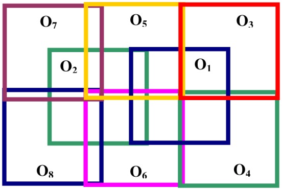
Protocol for sample image acquisition. This montage involves 8 partially overlapping OCT data sets for a given eye.

Our goal is to merge the various OCT data sets into a single large, 3D OCT data set covering an extended retinal region. In order to achieve this we first register every pair of OFIs with sufficient overlap, using blood vessel ridges as described in [29,34]. A global alignment step then creates an initial OFI montage and the process is iterated, updating the registration constraints at every step. Once the OFIs are globally registered, a fairly straightforward process of resampling, interpolation, and cross-correlation can be used to merge the full OCT data sets.

2.1. Preprocessing

It is well known that it is possible to improve the contrast of various features in the OFI by the use of A-scan filters adapted to the retinal anatomy [9]. For our purposes we decided to use a quick and simple approach, based on the location of the intensity peaks in the A-scans, to obtain a rough, but satisfactory RPE segmentation. After some smoothing we can select essentially the second (from the top) large peak in the A-scan (with some error correction using a continuity constraint, as well as a spacing constraint between peaks; the details are not essential) as a surrogate RPE surface and use a window of 20 pixels above and 100 pixels below the surface to build the enhanced OFI (Fig. 2 ). In this context it is not crucial for the RPE segmentation to be extremely accurate and speed is a more important factor in the choice of algorithm.

Fig. 2.

Comparison between the OFI (sum of all intensities along the A-scans) and the enhanced OFI for two sample data sets. Panel A shows a typical B-scan. The same B-scan appears in B with a superimposed RPE segmentation line. C.1 and D.1 are the OFIs. C.2 and D.2 are the corresponding enhanced OFIs. Notice that our very simple algorithm can results in some artifacts (arrows), but its performance is quite satisfactory for the present purposes.

2.2. Registration between individual image pairs

We consider all pairs of OFIs (O_i,O_j) in our sample and select those with sufficient overlap. We will assume that our set of images is such that for each two images O_i and O_j in it there is a connecting chain of images between them, that is a series of images O_K1,…,O_Km, such that O_i = O_K1, O_j = O_Km, and each image in the chain has sufficient overlap with the image following it. Typically, an overlap of more than a quarter of the image area was defined to be sufficient overlap [33]. This requirement can be relaxed somewhat by using for instance some a priori information on the relative location of the images. For instance, when using a precise acquisition protocol like the one described in Fig. 1, we can be more efficient in covering the retina and use an approximately 20% overlap as sufficient.

For all pairs (O_i,O_j) with sufficient overlap we can compute a linear transformation T_j,i that registers T_j,i(O_j) with O_i directly, using the approach described in [29]. Blood vessel ridges (roughly the center lines of blood vessels) are detected. A ridge pixel in O_i and the ridge pixel in T_j,i(O_j) closest to it form a pair of matching pixels and a similarity function is introduced, based on a specially defined distance between pairs of matching pixels. The registration transformation T_j,i is obtained by minimizing this similarity function. For all other pairs, a (potentially not unique) transformation T_j,i can be defined indirectly using a connecting chain of images between them.

2.3. Global alignment

For simplicity we select O₁ as the anchor image: we keep this image fixed and register all the other images to it. Also the transformations T_j,1 will be simply denoted by T_j from now on. Based on the registration parameters T_j (j = 2,…,n) between the other OFIs and the anchor OFI, the transformed OFIs can be pieced together to construct a montage (see Fig. 3 ).

Fig. 3.

Global alignment for a simplified montage of three OFIs. (A) A direct registration relationship exists for two image pairs: (O_a, O_c), and (O_b, O_c). (B) Let O_a be the anchor, and construct a montage. (C) Consider every possible combination of overlapping image pairs, and identify matching point pairs for each. New registration constraints are introduced for the image pair (O_a,O_b).

We can now examine the overlap between images without sufficient overlap and define new registration constraints for these image pairs. These registration constraints are analogous to the ones used for the direct registration, i.e. a set of matching point pairs is determined on the region of overlap [27]. For a ridge pixel on the reference image, we find the closest pixel on the registered target image; if their distance (determined by the Euclidean distance and the difference between the normal directions of the two pixels along each of their vessel ridge curves [29]) is less than a given threshold (experimentally determined, about 0.4 degrees of FOV), the pair of pixels is a matching point pair and is included in the updated registration constraints.

We can now compute new transformations T_j using a global minimization of the distance between all the matching point pairs (the ones used in the direct registration and the additional new ones). Let (x,y) be a point in O_j and (X,Y) its image after the transformation T_j. We can write the linear transformation relationship T_j as:

$$[X,Y,1]=[x,y,1]T_j=[x,y,1]\left[\begin{array}{ccc}{a}_{1,j}& -a_{2,j}& 0\\ a_{2,j}& a_{1,j}& 0\\ a_{3,j}& a_{4,j}& 1\end{array}\right]$$

If (x,y) and (x',y') are the coordinates of a pair of matching points in O_i and O_j respectively, the global alignment problem involves minimizing the sum of the distances (over all pairs of matching points) between [x,y,1]T_i and [x',y',1]T_j. This is easily set up as a linear least square problem. Let ${\rm N}$denote the column vector of montage parameters with 4(n-1) parameters, i.e.

$${\rm N} ={\left({\text{A}}_{\text{2}},\dots ,{\text{A}}_n\right)}^{\text{T}}.$$

where A_j = $\left(a_{1,j},a_{2,j},a_{3,j},a_{4,j}\right)$, for j = 2,…,n, contains the 4 parameters defining the transformation T_j.

Let $M$ be a 2k by 4(n-1) matrix, $b$ a 2k column vector, where k is the total number of matching point pairs, and (x,y), (x',y'), be the coordinates, respectively in O_i and O_j, of the m-th pair of matching points. The (m-1)-th and m-th rows of $M$are given by the following matrix:

$$\left(\begin{array}{l}\cdots 0\cdots ,x,y,1,0,\cdots 0\cdots ,-x\text{'},-y\text{'},-1,0,\cdots 0\cdots \\ \cdots 0\cdots ,y,-x,0,1,\cdots 0\cdots ,-y\text{'},x\text{'},0,-1,\cdots 0\cdots \end{array}\right)$$

where the only non zero blocks start at the (4i-3)-th and (4j-3)-th position. The corresponding entries in $b$are 0s. (The entries in M and b are slightly different when one of the indexes i, j is equal to 1. We leave the easy adjustments to the reader). The parameters for the global montage ${\rm N}$can be obtained as the least square solution to the linear system

$$MN=b$$

This global alignment is iterated several times (3 in our experimental setting) updating the registration constraints after each iteration. This iterative procedure is a kind of iterative closest point (ICP) algorithm.

2.4. 3D registration

Once we have obtained a montage of the OFIs, we can use it to piece together the full OCT data sets using a procedure based on resampling, interpolation, and cross-correlation. Let x and y be coordinates in the en face plane, defined by the axes of the anchor OFI O₁ (with x along the instrument scanning direction), while z denotes the coordinate in the axial direction. Let R be a rectangle in the x-y plane covering the entire OFI montage and with sides parallel to the x and y axes. We can then define a set of n+1 (where n is the number of OCT data sets) connected, non overlapping regions R_j such that R_j is contained in T_jO_j for j = 1,...,n and R₁ $\cup \cdots \cup$R_n+1 = R. A new global sampling grid s_ij (where the second index runs along the x direction) over R is generated by extending homogeneously the orthogonal sampling grid of the anchor image. The montage OCT is built by defining an A-scan for each point in the grid s_ij.

Let m₁, m₂ be the dimensions of the grid over R. For each given value of i, 1≤i≤m₁, let B_i be the B-scan over s_ij, for j = 1,…,m₂. For the sake of simplicity we can assume that B_i only intersects R₁ and R₂, i.e. s_ij $\subset$R₁ for j = 1,…,m and s_ij $\subset$R₂ for j = m+1,…,m₂. Then essentially the first m A-scans in B_i can be obtained using a weighted closest point interpolation of the A-scans in I₁ and the rest by a weighted closest point interpolation of the A-scans in I₂. In order to have the A-scans match smoothly across the transition some consistency constraints are needed. We define a transition region (a few grid points around s_im which are contained both in T₁O₁ and T₂O₂) and at each point in this region we use cross-correlation to find the optimal shift that matches the A-scan in I₂ with the corresponding A-scan in I₁. A linear fit of the shifts in the transitional region is used to compute shifts over s_ij for j=m+1,…,m₂. This approach can be extended in a straightforward manner to the case when a B-scan intersects several or the sets in the partition of R and, correspondingly, multiple transitional regions.

3. Experimental Results

We tested the algorithm in this paper using an imaging protocol that consisted of 8 partially overlapping OCT data sets as shown in Fig. 1. For each eye, the 8 OCT data sets were acquired in a single imaging session, using a Cirrus HD-OCT (Carl Zeiss Meditec Inc, Dublin, California). Each data set consisted of a raster scan covering a 6 X 6 mm area with 200 X 200 A-scans. The scans O₁ and O₂ are centered at the fovea and the optic disc respectively (or vice versa, depending whether it was a right or left eye). The total retinal area covered is approximately 50x35 degrees. Approval for the collection and analysis of SDOCT images was obtained from the Institutional Review Board at the University of Miami Miller School of Medicine and all participants signed research informed consent.

We analyzed the sets of OCT images of 3 normal eyes and 3 eyes with retinal degeneration. Figure 4 shows the results of the montage algorithm on the OFIs for one normal eye and eye with retinitis pigmentosa, while Fig. 5 shows a B-scan in the OCT montage of a normal eye.

Fig. 4.

Example montage results of enhanced OFIs for one normal eye (left) and one eye with retinitis pigmentosa (right).

Fig. 5.

OFI montage (left) and a B-scan (right) from the corresponding OCT montage. The position of the B-scan is shown by the red horizontal line. The width of the transition regions is a single pixel.

Registration errors are measured by calculating the average root mean square error (RMSE) of manually labeled matching point pairs. Matching point pairs are normally blood vessel branching points, and we manually label all point pairs that can be identified, typically several point pairs for each image pair (see [29]). Using our imaging protocol we have 13 (non trivially) overlapping image pairs. Table 1 shows the means and standard deviations of RMSE values for the individual image pairs, as well as for the whole montage.

Table 1. Averages and standard deviations (within parentheses) of RMSE values (in pixels) for the different image pairs as well as the whole montage. For our data sets a pixel corresponds to 30 µm.

	7&5	7&2	8&2	8&6	2&5	2&6	2&1	5&3	5&1	6&4	6&1	1&3	1&4	all
Normal Eyes	1.9 (0.7)	1.6 (1.0)	1.6 (1.2)	2.0 (1.4)	1.4 (0.6)	1.2 (0.4)	1.7 (0.7)	1.2 (0.5)	1.1 (0.4)	1.0 (0.9)	1.5 (0.5)	1.2 (0.6)	1.7 (0.8)	1.5 (0.3)
Diseased Eyes	0.9 (0.8)	1.4 (0.3)	2.1 (2.4)	6.5 (4.9)	1.5 (1.0)	2.5 (1.4)	2.3 (0.2)	2.4 (0.3)	1.2 (0.8)	0.9 (0.2)	1.9 (1.1)	0.8 (0.3)	1.3 (0.5)	2.0 (0.8)

4. Discussion and Conclusion

SD-OCT can acquire 3D retinal images whose FOV is limited by the scanning speed of the instrument. This paper proposes an automatic algorithm for the montage of 3D OCT data sets. Our algorithm merges together a number of partially overlapping OCT data sets to form a new, wide-field, 3D OCT data set. Although there is an extensive literature related to the montage of images, including traditional retinal images such as color fundus photographs, to the best of our knowledge this is the first work on the montage of OCT data sets or even OFIs. Our algorithm was tested on data sets consisting of 8 OCT images, covering a total FOV of about 50x35 degrees. We measured registration errors of 1.5±0.3 and 2.0±0.8 pixels for 3 normal eyes and 3 eyes with retinal degeneration, respectively.

The core of our montage algorithm is a 2D montage algorithm for OFIs. The 2D montage algorithm is similar to the one in Yang et al. [23], which addresses the montage of traditional retinal images such as color fundus photographs. For the specific application to OFIs, the choice of registration feature can be somewhat problematic. Blood vessel ridges are selected here as registration feature due to their relative stability [29]. However, standard OFIs can sometime show (areas of) poor blood vessel contrast which, when used in the montage algorithm, can lead to incorrect results. In order to overcome this problem, we use a simple and efficient approximate RPE boundary detection, and enhance the OFIs by filtering out the OCT intensities away from the segmentation. Of course a more sophisticated RPE segmentation algorithm [35–37], and/or filtering approach, could be used here, but we did not want to introduce unnecessary complexities and, although our segmentation algorithm is very basic, the resulting OFIs show a sufficient improvement in contrast for our purposes.

Yang et al. [23] did not update the constraints for the image pairs that were registered directly (step 2.2), because they claimed that the pairwise constraints are sufficient for accurate results in the joint alignment step. This does not appear to be the case for the application to OFIs. Hence, we update registration constraints for every image pair with overlap. In addition, the ICP is used instead of the CDC in [23], to save computation time. In practice information about the approximate location of an OCT data set with respect to fixed retinal landmarks is stored during image acquisition and could be available to the montage algorithm, therefore the improvement in convergence domain associated with CDC was not considered a crucial feature.

Eye movements during acquisition are an important factor producing artifacts/distortions in OCT data sets. These types of artifacts are often easily recognizable in the OFIs and the affected data sets can be discarded by a skilled operator during the imaging session. In principle it would be possible to split a data sets marred by eye-motion artifacts in several artifact free pieces and (as long as the single pieces contained enough recognizable features) use these pieces as input for the montage algorithm.

When building the full OCT montage (step 2.4) there are typically several different possible choices for the partition R₁ $\cup \cdots \cup$R_{n + 1} = R. Different choices of partition sets will result in slightly different OCT montages. Normally these differences are non essential (equivalent to taking two different OCT images of the same eye), but there are situations when the choice of one OCT image has definite advantages over its competitors on a region of overlap, i.e. better image quality, absence of artifacts, etc. In these cases it can make sense to pursue an optimal choice of partition. One possible way to accomplish it is by defining weights over (regions of) each individual OFI. These weight could incorporate both objective information (image quality scores, local OCT intensity values) and subjective judgment from the operator.

During image acquisition, factors like the beam entrance point in the pupil and the location of the fixation target can influence considerably the retinal tilt in the imaging cube. It is then reasonable to be concerned about possible higher order discontinuities (kinks in the retinal geometry) in the OCT montage across the boundaries of the partition sets. Our definition of transition regions is meant to perform a first order correction for this potential issue by introducing an additional linear adjustment of the imaging plane in each individual OCT data set. In practice though it turns out that it is almost always sufficient (at least in our experience, operator’s skill and other factors may play a role) to consider transition regions of width equal to a single pixel, corresponding to a zero order correction of the imaging plane (i.e. a simple uniform shift in the z-direction across each OCT data set).

The ability to montage OCT data sets implies the possibility to piece together any kind of information about the underlying OCT data sets. For instance it is certainly possible to extend segmentations maps of each OCT data sets to the montage. Figure 6 shows the retinal thickness maps for the OCT montage of a normal eye obtained from the individual retinal thickness maps.

Fig. 6.

Retinal thickness maps montage for a normal eye.

The algorithm was realized in MATLAB. No effort was made to optimize for speed. Given a set of 8 OCT data sets, as described in Fig. 1, the computation time for the montage was approximately 8 minutes.