A comparative assessment of univariate longevity measures using zoological animal records

Summary

Comparative biogerontology evaluates cellular, molecular, physiological, and genomic properties that distinguish short-lived from long-lived species. These studies typically use maximum reported lifespan (MRLS) as the index against which to compare traits, but there is a general awareness that MRLS is not ideal due to statistical shortcomings that include bias resulting from small sample sizes. Nevertheless, MRLS has enough species-specific information to show strong associations with many other species-specific traits, such as body mass, stress resistance, and codon usage. The major goal of this study was to see if we could identify surrogate measures with better statistical properties than MRLS but that still capture inter-species differences in extreme lifespan. Using zoological records of 181 bird and mammal species, we evaluated 16 univariate metrics of aging and longevity, including non-parametric quantile-based measures and parameters derived from demographic models of aging, for three desirable statistical properties. We wished to identify those measures that: 1) correlated well with MRLS when the biasing effects of sample size were removed; 2) correlated weakly with population size; and 3) are highly robust to the effects of sampling error. Non-parametric univariate descriptors of the distribution of lifespans clearly outperformed the measures derived from demographic analyses. Mean adult lifespan and quantile-based measures, and in particular the 90^th quantile of longevity, performed particularly well, demonstrating far less sensitivity to small-sample size effects than MRLS while preserving much of the information contained in the maximum lifespan measure. These measures should take the place of MRLS in comparative studies of lifespan.

Introduction

Aging is a process that gradually impairs vigorous mature adults and renders them more susceptible to a wide range of diseases and disabilities, leading to a progressive increase in mortality risk. Maximum recorded lifespan (MRLS) is the standard comparative metric used in experimental and observational research into the causes of aging (Comfort 1979; Austad & Fischer 1991; Holmes & Austad 1995; Wilkinson & South 2002; Hulbert et al. 2007), and it is often taken as the key endpoint in comparisons among species, genotypes, or groups exposed to different environmental manipulations. Comparative biogerontologists have long made use of MRLS as a surrogate for species-specific aging rate, and much effort has gone into compiling tables of MRLS values for this purpose (Finch 1990; Carey & Judge 2000; de Magalhaes & Costa 2009).

It is widely appreciated, however, that MRLS is a problematic indicator for several reasons. First, MRLS is a downwardly biased indicator of extreme lifespan. As sample sizes increase, expected MRLS values are expected to increase as well. Second, the sample variance associated with estimates of population MRLS may be high, especially with small sample sizes. These two issues may present serious problems in comparative studies involving rare non-laboratory animals. Consequently, MRLS may differ across species owing to differences in the number of species records used to determine longevity as well as to inherent differences in the physiology and ecology of the species. Third, MRLS does not use data effectively in situations where records are incomplete, which is often the case in many observational studies where the terminal recorded event for an individual may not be death (i.e., right-censoring). Lastly, it reflects lifespan of a single individual per species, grossly overestimating the characteristics of other members of the species. Given the concern that some record-breaking lifespans may be exaggerated (Steven Austad, pers. comm.), such extreme dependence on single outliers is undesirable.

Other metrics have been introduced in attempts to improve upon MRLS by applying multivariate demographic models of aging, such as Gompertz or Weibull functions, to survival data (Promislow 1991; Wilson 1994; Ricklefs & Scheuerlein 2002). In some cases, these parameters have been assigned controversial biological interpretations, as, for example, when the slope of a Gompertz plot is interpreted as a measure of the rate at which aging occurs (Finch et al. 1990; Pletcher et al. 2000; Bronikowski et al. 2011), and the intercept of a Gompertz plot is interpreted as the inherent frailty of the members of the population (Spencer & Promislow 2005; Maklakov et al. 2006; Flatt & Kawecki 2007). In other cases, parameter estimates derived from these models are combined, for example by multiplication, to arrive at a univariate summary of aging rates (Ricklefs 1998; Ricklefs & Scheuerlein 2001). Non-parametric methods have also been proposed that summarize the lifespan distribution of an elite subset of the population into quantiles and/or means (Wang et al. 2004; Gao et al. 2008). One significant advantage of these alternative methods over MRLS is that their application is not limited to the empirical distributions of complete lifespans; they can benefit from the use of the Kaplan-Meier estimator, which allows the use of censored data. Each of these estimators, and their combinations, has only an indirect relationship to the underlying biological processes of aging, and it is unclear how well these longevity metrics perform compared to MRLS as an index of differences of the pace of age-related change among biologically interesting populations.

Questions about the evolution of different aging rates and the cellular and molecular processes that can lead to striking differences in longevity among related species are the central arena for comparative biogerontology. Within orders of mammals, MRLS values among species of rodents or primates can vary 4- to 8-fold. Many evaluations of hypotheses about comparative aging among species have depended on MRLS as the index of inter-species differences in aging rate, despite the measure's well-known defects. Our goal in this project was to make use of population data, obtained from zoo populations of nearly 200 bird and mammal species, to explore the sampling properties of various univariate aging and longevity metrics. Some of these metrics have been proposed by others, but some have not previously been applied to questions in the comparative biology of aging. We wished to understand how well each measure indicates extreme lifespan across a phylogenetically diverse range of species that differ in life history and data quality. In addition, we wanted to understand how robust each metric is to sampling effects, namely sampling variance and bias arising from small population sizes. A major goal of this study was to understand the limitations of MRLS as a comparative longevity metric and, if possible, identify an alternative measure for MRLS that minimizes the sampling issues and data-use restrictions associated with that measure.

The datasets available to test hypotheses in the comparative biology of aging differ in the proportion of missing values and in the extent of erroneous data. The data often combine records from wild and captive populations that differ in environmental factors (housing conditions, food availability, reproductive histories, predation and infection levels, etc.) that can have strong effects on mortality risks through both age-dependent and age-independent pathways. Although tables of MRLS values across species contain a good deal of information critical to testing ideas about the biology of aging, there is a pressing need to develop improved demographic endpoints for biogerontology.

Results

Onset of aging

Although it is not clear whether the aging process begins at any defined life history transition (birth, puberty, age at first reproduction), we assume here that deaths at the earliest ages, for example perinatal deaths and deaths of juveniles, are unlikely to be informative about inter-population variances in aging rates. We therefore used two methods to determine the age before which mortality should be ignored, and we report the results derived from both methods. We analyzed the subset of individuals from each species with events (deaths or last observations) that met or exceeded one of two species-specific truncation ages: 1) T_1, the age of reproductive maturity for that species, or 2) T_2, the age at which the mortality rate reaches a minimum (see Table S1 for species, relevant life history information, and T estimates). Across the 163 species that had at least 50 adults defined by both threshold definitions (T₁ and T₂), the truncation ages correlated reasonably well (ρ = 0.53, p < 0.0001, Spearman's rank correlation; see Figure 1). Nearly two-thirds of the species with both T₁ and T₂ estimates had an age at minimal mortality that exceeded the age at reproductive onset (108 of 163 species). This pattern is consistent with Promislow's (1991) earlier analysis of a much smaller set of species records in which he showed T₁ < T₂ in 75% (18 of 24) of cases where age at maturity and age at minimal mortality differed. More recent life history analyses also show that the onset of aging tends to follow the timing of reproductive maturity (Jones et al. 2008; Peron et al. 2010). The correlation between T₁ and T₂ estimates strengthened slightly when the collection of species was reduced to include only the 125 species with 150 or more adults (ρ = 0.58, p < 0.0001). While the positive correlation was encouraging, it seemed prudent to analyze the sampling properties of the various metrics using each T-definition independently. As we show below, however, the choice of T-definition had little effect on the sampling properties of the metrics.

Figure 1. Two methods of determining age of onset.

shows the joint distribution between 1) the oldest of the two sex-specific values for the first age of reproduction and 2) age at minimal mortality for 163 species with 50 or more adults (as defined by both definitions). The line defines the T₂ = T₁ relationship.

Metric estimates

Using both threshold definitions, we estimated sixteen univariate longevity values (defined in Table 1) for each of the 175 (T₁) and 165 (T₂) species, respectively, that had at least 50 adult individuals (as defined by each T-definition) with recorded events (Supplement Tables S2A and S2B). For a few cases of the T₁ treatment, the Weibull function failed to converge. This may have resulted from too few adult deaths in the dataset (Ricklefs 1998) or from inclusion of part of the early age range typified by elevated mortality (by definition, this would not be a problem using the T₁ criterion).

Table 1.

Univariate longevity metrics

	Parametric?	Details
MxLS	no	Mean lifespan of the x longest-lived individuals x=1,4,8,16, 32 (where M1LS represents MRLS)
GA	yes	intercept of the maximum likelihood Gompertz model (μ = AeBx)
GB	yes	slope of the maximum likelihood Gompertz model
WA	yes	intercept of the maximum likelihood Weibull model (μ = AxB)
WB	yes	slope of the maximum likelihood Weibull model
Ω	yes	Omega index based upon a Weibull model Ω = A1/(B+1)
QX	no	The xth lifespan quantile x = .5, .9, .95
e x	no	The mean lifespan above the xth lifespan quantile x = 0, .9, .95

Correlations among metrics

We correlated estimates across species using both truncation methods (Table 2) holding population size constant (a full correlation matrix, in which sample size is not corrected for, is presented in Table S3 of the Supplemental Information). In general, the nonparametric measures of lifespan were highly correlated among each other (0.869 or better). Except for the mean (e₀) and median lifespan (Q₅₀), the lowest partial correlations among non-parametric estimators were between MRLS and Q₉₀ (0.950 for T₁ and 0.941 for T₂). The partial correlation between MRLS and Q₉₅ was also 0.950 using the T₁ criterion but higher (.957) for T₂. With the exception of the Weibull intercept, W_A, and Ω (a function of the slope and intercept of the Weibull model), parametric measures of mortality correlated negatively with MRLS and the other nonparametric measures of longevity. This is to be expected, because these are aging parameters, and aging and longevity are negatively associated. Of these, only the Gompertz and Weibull intercepts (G_A and W_A) correlated reasonably well with MRLS (-0.789 and -0.698 for G_A and -0.928 and -0.938 for W_A). Slopes and intercepts were poorly correlated for both the Gompertz and Weibull models. Independence between G_A and G_B estimates has been previously recently reported across eight primate species (Bronikowski et al. 2011).

Table 2.

Partial correlations using ISIS species data, holding sample size constant

MRLS	.992	.986	.977	.964	-.789	-.570	-.928	.280	-.238	.883	.950	.950	.927	.973	.980
.991	M4LS	.997	.991	.980	-.802	-.563	-.937	.297	-.223	.890	.961	.974	.936	.984	.990
.983	.997	M8LS	.997	.989	-.808	-.550	-.936	.314	-.204	.896	.967	.977	.941	.986	.990
.970	.989	.996	M16LS	.996	-.817	-.534	-.938	.331	-.186	.905	.973	.980	.950	.986	.988
.958	.980	.989	.997	M32LS	-.825	-.511	-.934	.348	-.168	.913	.975	.977	.955	.981	.979
-.698	-.719	-.727	-.739	-.755	GA	.148	.880	-.641	-.143	-.912	-.856	-.842	-.902	-.837	-.824
-.733	-.718	-.704	-.681	-.652	.186	GB	.627	.390	.779	-.270	-.485	-.522	-.373	-.533	-.550
-.938	-.948	-.947	-.946	-.942	.828	.628	WA	-.300	.243	-.912	-.951	-.959	-.940	-.957	-.953
.120	.148	.162	.185	.217	-.635	.452	-.206	WB	.811	.522	.378	.345	.462	.336	.314
-.297	-.273	-.258	-.234	-.201	-.252	.770	.230	.877	Ω	.028	-.141	-.176	-.045	-.187	-.209
.869	.883	.889	.901	.913	-.858	-.442	-.914	.421	.027	Q50	.939	.919	.986	.921	.907
.941	.956	.964	.972	.975	-.793	-.604	-.956	.244	-.170	.947	Q90	.991	.978	.990	.979
.957	.973	.979	.983	.983	-.773	-.643	-.959	.214	-.204	.930	.994	Q95	.965	.997	.993
.907	.922	.928	.937	.945	-.844	-.511	-.941	.362	-.044	.991	.974	.963	e0	.966	.954
.971	.982	.985	.985	.981	-.766	-.633	-.963	.195	-.224	.924	.990	.997	.958	e90	.997
.981	.990	.989	.984	.977	-.748	-.690	-.961	.170	-.251	.907	.976	.989	.944	.996	e95

Each cell gives the partial correlation between two measures of longevity taken over ISIS species, holding sample sizes constant. The diagonal cells define the measures. Elements above the diagonal report the corresponding partial correlation using the T₁ truncation method and those below use the T₂ method. For example, the cell at row 1, column 2 is the partial correlation between MRLS and M4LS, which is .992 using T₁. Using T₂, the cell at row 2 and column 1 indicates that correlation between these measures is .991. Shaded cells indicate metric pairs where the absolute value of the partial correlation coefficient is at least 0.95.

Correlations between metrics and population sizes

We correlated metric estimates with population sizes (n) using both T₁ and T₂ criteria (Figure 2). In most cases, metrics that were estimated using T₁ were less strongly associated with n than those estimated using T₂. As expected, we found positive correlations between n and MRLS (+0.105 and +0.162). Positive correlations increased with increasing x in MxLS (the mean lifespan of the x longest-lived individuals), reaching +0.276 and +0.312 with M32LS. For these metrics, the T₂ treatment yielded slightly greater correlations that the T₁ treatment. With the exception of W_A, parametric measures were very sensitive to the choice of T. The Weibull and Gompertz slopes, as well as the Weibull omega measure, yielded moderately negative correlations with n in the T₂ treatment (-0.358, -0.480, and -0.480, respectively). Using T₁, however, these correlations remained negative but markedly decreased in magnitude (-0.039, -0.127, and -0.089). The Weibull and Gompertz intercepts were weakly and positively correlated with population size, except for G_A estimated with T_2, which was the highest correlation that we observed (+0.313). Promislow et al (1999) also report little association between Gompertz parameters and population size in simulated populations using a defined age of onset (similar to our T₁ treatment). The more extreme quantile-based measures (Q₉₀, Q₉₅, e₉₀, and e₉₅) showed the weakest associations with sample size (correlations ranged between -0.037 and +0.018). The measures of central tendency (Q₅₀ and e₀) correlated weakly and negatively with n using T₁ (-0.066 for both) and correlated more strongly with T₂ (-0.174 and -0.147). Correlations involving these measures, and using either T₁ or T₂, most closely resembled those generated from the extreme quantile-based measures.

Figure 2. Correlations between longevity metrics and population size.

illustrates the correlations between candidate metrics and population size. Correlations are sensitive to the definition of adult (T) used to estimate the measures. For each measure, bars connect the T₁ and T₂-derived estimates. Long bars indicate high sensitivity of the correlation to the choice of T.

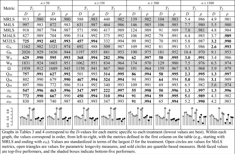
Rank persistence

We next asked how finite population size affected the ranking of lifespan metrics across all study species. Every population (for our purposes, a population was considered the worldwide collection of animals of the same species, and we use species and population interchangeably) was re-sampled n_i times with replacement, where n_i was each species’ sample size, and each species was ranked in order of each longevity value (resulting in 16 metric-specific ranking vectors). For example, a MRLS vector may be ordered species A > species B > species C > species D and a W_A vector may rank species B > D > A > C. This procedure was repeated, and each pair of metric-specific ranking vectors was analyzed for stability. Rank persistence, as inferred by a low Spearman's Footrule Distance D and a high Spearman's ranked correlation coefficient ρ, quantified how robust each measure was to sampling variation. We investigated four population size treatments. The n ≥ 50 treatment included all species populations with at least 50 observed adult deaths (n_T1,50 = 175, n_T2,50 = 165). We performed three other rank persistence analyses using the same resampling approach, except that we made the minimal sample size requirement more stringent each time. We considered species with n ≥ 150 (n_T1,150 = 147, n_T2,150 = 126), n ≥ 500 (n_T1,500 = 66, n_T2,500 = 56), and n ≥ 1500 (n_T1,1500 = 15, n_T2,1500 = 13). Note that the treatments differed only in the choice of which species to use; any species chosen for a treatment had all of its individuals included in the analysis. Rank persistence averaged over 1000 resampled population pairs is described in Table 3. For each treatment, robustness measure, and T-definition, the five most persistent metrics are indicated in boldface and the five least persistent metrics are shaded.

Table 3.

Rank persistence analysis (fixed population size)

In general, the non-parametric estimators outperformed the parametric estimators in nearly every treatment. The sole exception was that the Weibull intercept W_A was a frequent top-five performer. The Gompertz intercept G_A performed well at the highest population size treatment using the T₂ definition. G_B, W_B, and Ω were always among the least persistent metrics. Of the nonparametric estimators, the quantile-based approaches demonstrated the most persistence. This was especially evident in the metrics that described central tendency (e₀ and, to a lesser degree, Q₅₀). More extreme values of longevity, Q₉₀ and e₉₀, also performed very well across all treatments. The M32LS method performed very well at low sample sizes but less so at the n ≥ 500 and n ≥ 1500 treatments.

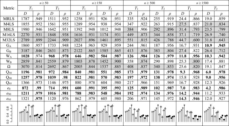
All of the metrics under consideration are subject to sample size bias. For this reason, we reasoned that the species rankings reflected both inherent differences in the biology of species as well as variation in the size of the pooled zoo animal population datasets provided by ISIS. We note that datasets available for testing hypotheses about species differences in aging and longevity are also likely to contain a preponderance of small populations, similar in this way to the datasets available through ISIS. We attempted to remove the latter source of variation from our rank persistence analysis by randomizing sample size. As before, a rank persistence analysis was performed using populations with adult numbers of at least 50, 150, 500, and 1500 individuals. In this treatment, however, the resampling procedure was changed. Instead of taking n_i samples from each species i, the number of samples was randomized; the exponential of some uniformly distributed number of samples x_i were drawn with replacement over the interval ln(50) ≤ ln(x_i) ≤ ln(n_i) (this sets the range at between 50 and n_i with most samples near the low end of the range). As before, adults were those individuals with terminal events (deaths or last observations) defined by T₁ or T₂ and rank persistence was quantified by D and ρ. Mean persistence values are shown in Table 4.

Table 4.

Rank persistence analysis (randomized population size)

The randomized treatments demonstrated weaker rank persistence. This is what we would expect if randomizing sample size eliminated that component of the fixed species rank determined by population size. This was consistent with our goal of removing sample size as predictor of longevity. In general, the quantile-based nonparametric estimators appeared to preserve rank best, although the Weibull intercept W_A again showed relatively high rank persistence. Interestingly, the relative advantage of these nonparametric estimators over the alternatives appeared to be greater with randomized population sizes. This finding suggests that sample size variation has a greater effect on parametric measures of longevity than on non-parametric measures. As before, W_A and the more intermediate quantile measures, Q₅₀ and e₀, performed best and Q₉₀ and e₉₀ performed next best. As a group, parametric methods continued to appear to be the worst performers (excepting W_A). At high sample sizes, however, the Gompertz intercept G_A performed relatively well, providing species ranks that were roughly as persistent as the quantile-based measures. The largest change in relative performance involved nonparametric measures M16LS and M32LS; these were middling-to-good performers with fixed populations sizes but very poor performers when sample sizes are randomized. It appeared that for metrics MxLS, increasing x made for better metrics when samples sizes were fixed but worse metrics when sample sizes varied. This makes sense when we consider that, in terms of population lifespan quantiles, MxLS has different meanings as population size changes. Using unrealistically low population sizes to illustrate this point, MRLS is Q₉₅ in a population of 20 but equal to Q₅₀ (the longevity median) in a population of two.

Results were largely unaffected by our choice of T-definitions and persistence metric (D or ρ). In no case did altering these choices change a top-five performing metric (in terms of rank persistence) into a bottom-five performer. Ranked correlations between D and ρ values were very high in all population size treatments and using both T-definitions, with ranked correlation coefficients among persistence measures ranging between 0.941 and 0.988 (Table 5, “fixed” and “D and ρ” headings; “fixed” refers to the condition of this treatment where population sizes are preserved and not randomized, as in the following treatment). Likewise, persistence values were highly correlated across T-definitions. Ranked correlations ranged from 0.950 to 0.994 (Table 5, “fixed” and “T₁ and T₂” headings) in the three treatments with lowest population sizes. In the highest population size treatment, n ≥ 1500, the ranked correlations ranged somewhat lower, 0.721 and 0.812.

Table 5.

Sensitivity of metric performance to treatment and assessment changes

population size	fixed				random
	D and ρ		T1 and T2		D and ρ		T1 and T2
	T 1	T 2	D	ρ	T 1	T 2	D	ρ
n ≥ 50	.950	.979	.994	.965	.950	.979	.994	.976
n ≥ 150	.968	.985	.974	.950	.976	.988	.988	.982
n ≥ 500	.982	.988	.976	.950	.979	.997	.997	.976
n ≥ 1500	.941	.974	.812	.721	.965	.994	.956	.891

Discussion

A wide range of bird and mammal species have evolved that differ widely in life histories, including variation in the rate at which aging leads to increased risks of mortality due to disease and infirmity. This rich set of related species could, in principle, be used to generate and evaluate hypotheses about the cellular and physiological factors that time the aging process, factors that make it very unlikely that a particular mouse will survive 5 years, a dog survive 20 years, and a human survive 110 years. Lifespan is a convenient, if flawed, surrogate for addressing hypotheses about the biological basis for aging rates because many factors besides age change can lead to death, and because aging leads to many consequences in addition to changes in mortality risk. Ideally, hypotheses about the distribution of aging rates and age-dependent changes across species could be tested by a database in which multiple age-sensitive traits had been tested in hundreds of individuals across a wide range of diverse species. In practice, however, physiological data of this kind are available only for a handful of species, and for most species the only available data relevant to questions of comparative aging rate are in the form of survival tables. The obvious problem is to determine the best way to summarize these population–specific tables and provide a comparative metric that preserves relevant biological information relating to lifespan while disregarding the effects of extraneous or confounding factors, such as population size.

Despite the widespread appreciation of its statistical association with population size, the maximum recorded lifespan (MRLS) is favored by comparative biologists because it is believed to measure an individuals’ intrinsic potential for long life. The degree to which the other metrics measured this maximum, without regard for the biasing effects of small sample size, is quantified by the partial correlations between candidate metrics and MRLS, holding population size constant. Population size bias is addressed more directly by the total correlation between sample size and metric value. Ideally, the best measures of extreme lifespan are those with the greatest magnitude of partial correlations with MRLS and the least magnitude of the total correlation between the measure and sample size. By these criteria, the best are those that nonparametrically define some well-defined elite fraction of the population: Q₉₀, Q₉₅, e₉₀, and e₉₅. Given that adult lifespans are typically right-skewed, we expected that measures of central tendency should be affected least by sample size. Instead, we found negative correlations between these measures and n that were slightly stronger than those obtained from Q₉₀, Q₉₅, e₉₀, and e₉₅. Good evidence has been collected to suggest that animal size and lifespan are positively associated. If zoos favor larger collections of smaller animals (a feasible expectation given resource limitations), then these negative correlations between n and mean and median lifespans may reflect true associations between intrinsic aging and population size and not simply bias. Such associations would cause effects that act in opposition to the effects of sample size bias on MRLS estimates. Put differently, maximum recorded lifespan would be more sensitive to n than reflected by our correlation estimate. We note, however, that regardless of whether we choose the ideal correlation to be zero or slightly negative, Q₉₀, Q₉₅, e₉₀, and e₉₅ still appear to best satisfy these criteria for best longevity metrics.

Because MRLS observations depend upon the identification of single individuals, it seemed reasonable to expect that estimates would suffer from high sampling error. Indeed, our re-sampling analysis indicated that MRLS had a larger sampling variance than the quantile-based measures at all sample sizes. The difference intensified when species were disassociated from population sizes, suggesting that small sample bias may contribute to the sampling error for MRLS. Most parametric estimates suffered from high sample variance. The quantile-based measures produced the most reliable estimates, especially when population sizes were allowed to vary. Excluding those that describe the central tendency, we see that the least extreme measures Q₉₀ and e₉₀ are the least variable.

The 90^th quantile of adult lifespan, Q₉₀, and the average of the top 10^th percentile of adult lifespan, e₉₀, appear to be the best alternatives to using MRLS as a comparative metric for extreme lifespan. Both correlate well with MRLS when sample size is corrected for, correlate weakly with population size, and demonstrate relatively little sampling variance. Furthermore, both can accommodate right-censored data. Neither measure seems to have a clear advantage over the other based upon the sampling characteristics analyzed here. However, one may prefer Q₉₀ over e₉₀ if extreme lifespan exaggeration was considered to be a problem, because Q₉₀ is expected to be more robust to this effect than e₉₀. We recommend that future aging studies consider using the 90^th quantile lifespan as a comparative metric.

The metrics that took the average of a set number of elite individuals (MxLS) performed poorly as candidate metrics for extreme lifespan. Not surprisingly, MxLS measures correlated extremely well with MRLS when population size was held constant. However, the positive correlation between the measure and population size increased for this family of measures. Our rank persistence analysis illustrated problems inherent in the use of MxLS as a comparative metric. When population sizes were not randomized, MRLS and the closely related M4LS performed well, as indicated by high rank persistence to resampling. Similar methods that correlate well to MRLS (M16LS and M32LS) also performed well under these conditions. However, when population sizes were randomized to decouple the effects of biology and animal collection size, these performed very poorly compared to other measures. The reason for this is evident if we recognize that MxLS is the mean of the top 1 – (n-x)/n percentile of the population. Because the threshold for inclusion is sensitive to population size, variation in population size varies the lifespans of the individuals included in the measure.

Judged as univariate descriptors of longevity, measures based upon parameterized demographic models performed poorly as a group, with the exception of the Weibull intercepts, W_A. Estimates of these metrics seemed to be more sensitive to our choice of method for delineating the aging and non-aging segments of each species life history. These metrics correlated poorly with MRLS, holding population size constant. With respect to the Weibull-based omega values, our results (using T₁ as our definition of adulthood, the partial correlation was -0.238 and the total correlation was -0.464) contrast sharply with a full correlation between and MRLS of -.83 across 150 captive vertebrate species recently reported by Ricklefs (2010b). At least two reasons may account for this discrepancy. First, our analytical methods differ: Ricklefs uses least-squares regression to fit a three-parameter Weibull model to death records at all ages (we use maximum likelihood to fit a two parameter model to adult events) and he does not consider right-censored observations (we do). Second, the numbers of animal records per species tend to be far greater in our study. If small sample sizes upwardly bias estimates of omega (this is speculation on our part), then the variance in sample size across species (such as both studies find) will generate excess negative correlations between omega and MRLS. The results from the rank persistence analyses suggested that the demographic parameters, especially those that describe the slopes of mortality functions, are subject to high sampling variance. The Weibull intercept, however, demonstrated high partial correlations with MRLS and low sampling variances. Our only reason for not recommending this measure is that it correlated more strongly with population size, which suggests that it is a more biased measure than some of the nonparameteric alternatives.

While much attention in comparative biogerontology focuses on measures of extreme lifespan, investigators might consider using measures of central tendencies instead. There are at several reasons for doing so. First, as we show here, mean adult lifespan exhibits the least amount of sampling variance. It is the most repeatable measure that we investigated. Second, compared to MRLS, there is far less association between population size and metric estimates. As we have argued, there is reason to believe that mean lifespan should be the measure that is least biased by small sample size. Third, mean lifespan is highly correlated with MRLS (correcting for population size), with a partial correlation coefficient of between 0.91 and 0.93. Other measures, such as Q₉₀, may perform better in this respect, but it appears that a great deal of the biological information that is parameterized by maximum lifespan is also expressed by the mean lifespan of those animals that live at least as long as the ages measured by T₁ and T₂. Last, the most familiar definitions and predictions of the evolutionary change of phenotypes from one generation to the next are expressed as changes in the means (Robertson 1966; Price 1970; Price 1972; Lande & Arnold 1983). In evolutionary biology, it is changes in the means, and occasionally the variances, of phenotypes that are nearly always the subject of study. We note, though, that the means and medians used for our calculations are for samples that exclude perinatal and a high proportion of juvenile mortality, and cannot be used to evaluate issues related to life expectancy at birth or proportions of offspring surviving to reproductive age.

Ultimately, the choice of whether to compare means or extremes may depend upon the nature of the comparative question that is under study. We recommend, however, that this decision is made explicit and justified by each study. Comparative biogerontologists have prepared extensive compilations of MRLS data, and for many meta-analyses MRLS may, unfortunately, be the only available measure currently available. Compilation of similar lists of Q₉₀ values and mean lifespans of animals surviving at least to T₁ or T₂, would be a worthwhile project for field biologists and zoo consortia to tackle as a service to aging research, and we recommend that such statistics be routinely included in reports about lifespan and aging in wild, captive, and experimental populations. In this respect, our study makes an important contribution by providing these estimates for nearly 200 bird and mammal species.

Experimental procedures

Obtaining animal records

We obtained records for 200 species of captive-born birds and mammals from the International Species Information System (ISIS), an international non-profit membership organization of zoos and aquariums. ISIS maintains an extensive database derived from over 800 zoological institutions in 77 countries, including life history information on over 2.4 million individual animals, of which over 1.5 million have exactly recorded birthdates. ISIS data has contributed to previous studies of demographic parameters related to lifespan evolution (Ricklefs 2000; Ricklefs 2010a; Ricklefs 2010b), in which the absence of predation in zoological settings was believed to be an advantage in determining intrinsic mortality rates. Because information in the ISIS database differs greatly among species in the number of individuals, the degree of right censoring, the extent of missing data, and the pooling of information from zoos of varying size and environmental characteristics, these data provide an excellent opportunity to compare statistical estimates of extreme longevity in a realistic context.

Animal records included sex, birth dates and death dates (or last recorded observations). Animals with unknown or estimated birth dates were removed from the analysis. We also removed all animals with life-spans that exceeded 120% of the maximum recorded lifespan as reported by AnAge (de Magalhaes & Costa 2009). We chose this value to allow for the possibility that the ISIS records included valid ages of animals that exceeded the AnAge values (many record-breaking individuals were identified), but we did not want to include records of animals that were suspiciously old. We used two methods (explained below) to determine the initial age of our analysis of aging (T) for each species. Most (181 species) had 50 or more individuals (n ≥ 50) with ages at death that exceeded T –values determined by one or both methods. These species (Supplemental Table 1) were chosen for further analysis.

Determining T

Populations from the ISIS datasets exhibited U-shaped mortality functions of age. The close monitoring of individual animals in the zoological setting, especially starting with birth or hatch, generates data on early mortality. As we were only interested in the distribution of lifespans that are associated with senescence, we discarded deaths that occurred before the onset of aging (T). This age was determined in two different ways: First, we ignored all deaths that occurred before the age of first reproduction as determined by the literature (see Table S1 in the Supplemental Information). When sex-specific ages of first reproduction were available and different, we took the greater of the two ages to be the truncation age (T₁) for both sexes.

The second method found the age at which mortality was minimized (T₂). For each reduced population, we used a simple iterative routine to find T₂:

1. We calculated L_X values using the ‘Survival’ package in R 2.11.0 (R Development Core Team 2011; Therneau & Lumley 2011). Individuals with known death dates (complete) and dates of last observation (right-censored) were used. We binned the population into groups of similar lifespans, defined by regular age intervals. The bin number is defined by the “Sturges” algorithm (Sturges 1926), where the number of classes is a function of sample size, N = 1+log₂(n). This function is commonly used to construct histograms.

2. The age mid-point of the class with the lowest mortality value was the provisional T₂ value.

3. A new population was defined by individuals from this class and those from either of the flanking classes.

4. We repeated steps 1-3 using the new population until age bins appeared with no deaths or until the Sturges function no longer returned more than two classes.

5. The estimate of the mortality minimum was the last meaningful T₂ value (Table S1).

Estimating metrics

We estimated longevity using the post-T (aging) populations. Longevity metrics were of two types. Non-parametric estimates were functions of longevity quantiles, based upon survival curves generated from the survival analysis described above. Parametric estimates derived from functions of Gompertz or Weibull parameters fit to each aging population. Model fitting was accomplished using the ‘Survomatic’ package in R 2.11.0 (Bokov & Gelfond 2010; R Development Core Team 2011). Metrics are described in detail in Table 1, and estimates are presented in Supplemental Table S2.

Rank persistence

We were interested in discriminating between populations represented by their longest-lived individuals. One way to evaluate the merits of candidate metrics is to perform rank persistence analyses of re-sampled species-specific populations. We began with a collection of P species, each of size N_p. We re-sampled each species twice with replacement, taking N_p draws from each population p. For each metric m, there was a ranking sequence specific to each sample set. For example, the MRLS rankings for five sample species (p = 1 to 5) may have been

$$\begin{array}{cc}\hfill R1(m=MRLS)& =\{1,2,3,4,5\}\hfill \\ \hfill R2(m=MRLS)& =\{1,3,4,2,5\}\hfill \end{array}$$

In this case, species 1 always has the longest-lived individual and species 5 always has the lowest maximum aged individual. Species 2, 3, and 4 exchange rank. Using the same re-sampled data, a metric other than MRLS might return rankings that are more persistent:

$$\begin{array}{cc}\hfill R1(m=X)& =\{1,3,2,4,5\}\hfill \\ \hfill R2(m=X)& =\{1,2,3,4,5\}\hfill \end{array}$$

We can quantify rank persistence using two slightly different measures. The first measure is Spearman's Footrule Distance: $D_{ij}={\sum }_{k=1}^n\mid x_{ik}-x_{jk}\mid$, where i and j are R1 and R2, x is the rank and k is the population. For the examples above, D_R1R2 (MRLS) = 4 and D_R1R2 (X) = 2. Persistence increases with decreased D (low values are superior to high values). The second measure is r_ij, the rank correlation across the samples, which increases with rank persistence (high values are superior to low values). In our example, r_R1R2 (MRLS) = +0.7 and r_R1R2 (X) = +0.9. Note that the measures are very similar; the only fundamental difference between the two measures is that r weights changes in rank by the square of the change and D scales the changes linearly. By both measures, the rankings derived using metric X would seem to more robust to changes in the populations resulting from re-sampling. In terms of rank persistence alone, we would conclude that X is a superior longevity metric to MRLS.

Literature Cited

- Austad SN, Fischer KE. Mammalian aging, metabolism, and ecology: evidence from the bats and marsupials. J Gerontol. 1991;46:B47–53. doi: 10.1093/geronj/46.2.b47. [DOI] [PubMed] [Google Scholar]
- Bokov AF, Gelfond J. Survomatic: Analysis of longevity dataed^eds) 2010.
- Bronikowski AM, Altmann J, Brockman DK, Cords M, Fedigan LM, Pusey A, Stoinski T, Morris WF, Strier KB, Alberts SC. Aging in the natural world: comparative data reveal similar mortality patterns across primates. Science (New York, N.Y. 2011;331:1325–1328. doi: 10.1126/science.1201571. [DOI] [PMC free article] [PubMed] [Google Scholar]
- Carey JR, Judge DS. Longevity Records: Monographs On Population Aging Vol 8: Life Spans Of Mammals, Birds, Amphibians, Reptiles, And Fish. University Press Of Southern Denmark; Odense: 2000. [Google Scholar]
- Comfort A. The biology of senescence. Churchill Livingstone; London: 1979. [Google Scholar]
- de Magalhaes JP, Costa J. A database of vertebrate longevity records and their relation to other life-history traits. Journal of Evolutionary Biology. 2009;28:1770–1774. doi: 10.1111/j.1420-9101.2009.01783.x. [DOI] [PubMed] [Google Scholar]
- Finch CE. Longevity, Senescence, and the Genome. University of Chicago Press; Chicago: 1990. [Google Scholar]
- Finch CE, Pike MC, Witten M. Slow mortality-rate accelerations during aging in some animals approximate that of humans. Science (New York, N.Y. 1990;249:902–905. doi: 10.1126/science.2392680. [DOI] [PubMed] [Google Scholar]
- Flatt T, Kawecki TJ. Juvenile hormone as a regulator of the trade-off between reproduction and life span in Drosophila melanogaster. Evolution. 2007;61:1980–1991. doi: 10.1111/j.1558-5646.2007.00151.x. [DOI] [PubMed] [Google Scholar]
- Gao GM, Wan W, Zhang SJ, Redden DT, Allison DB. Testing for differences in distribution tails to test for differences in ‘maximum’ lifespan. Bmc Med Res Methodol. 2008;8:49–58. doi: 10.1186/1471-2288-8-49. [DOI] [PMC free article] [PubMed] [Google Scholar]
- Holmes DJ, Austad SN. The evolution of avian senescence patterns - implications for understanding primary aging processes. American Zoologist. 1995;35:307–317. [Google Scholar]
- Hulbert AJ, Pamplona R, Buffenstein R, Buttemer WA. Life and death: Metabolic rate, membrane composition, and life span of animals. Physiol Rev. 2007;87:1175–1213. doi: 10.1152/physrev.00047.2006. [DOI] [PubMed] [Google Scholar]
- Jones OR, Gaillard JM, Tuljapurkar S, Alho JS, Armitage KB, Becker PH, Bize P, Brommer J, Charmantier A, Charpentier M, Clutton-Brock T, Dobson FS, Festa-Bianchet M, Gustafsson L, Jensen H, Jones CG, Lillandt BG, McCleery R, Merila J, Neuhaus P, Nicoll MAC, Norris K, Oli MK, Pemberton J, Pietiainen H, Ringsby TH, Roulin A, Saether BE, Setchell JM, Sheldon BC, Thompson PM, Weimerskirch H, Wickings EJ, Coulson T. Senescence rates are determined by ranking on the fast-slow life-history continuum. Ecol Lett. 2008;11:664–673. doi: 10.1111/j.1461-0248.2008.01187.x. [DOI] [PubMed] [Google Scholar]
- Lande R, Arnold SJ. The measurement of selection on correlated characters. Evolution. 1983;37:1210–1226. doi: 10.1111/j.1558-5646.1983.tb00236.x. [DOI] [PubMed] [Google Scholar]
- Maklakov AA, Friberg U, Dowling DK, Arnqvist G. Within-population variation in cytoplasmic genes affects female life span and aging in Drosophila melanogaster. Evolution. 2006;60:2081–2086. [PubMed] [Google Scholar]
- Peron G, Gimenez O, Charmantier A, Gaillard JM, Crochet PA. Age at the onset of senescence in birds and mammals is predicted by early-life performance. P Roy Soc B-Biol Sci. 2010;277:2849–2856. doi: 10.1098/rspb.2010.0530. [DOI] [PMC free article] [PubMed] [Google Scholar]
- Pletcher SD, Khazaeli AA, Curtsinger JW. Why do life spans differ? Partitioning mean longevity differences in terms of age-specific mortality parameters. The journals of gerontology. 2000;55:B381–389. doi: 10.1093/gerona/55.8.b381. [DOI] [PubMed] [Google Scholar]
- Price GR. Selection and covariance. Nature. 1970;227:520–521. doi: 10.1038/227520a0. [DOI] [PubMed] [Google Scholar]
- Price GR. Extension of covariance selection mathematics. Annals of Human Genetics. 1972;35:485–490. doi: 10.1111/j.1469-1809.1957.tb01874.x. [DOI] [PubMed] [Google Scholar]
- Promislow DEL. Senescence in natural populations of mammals - a comparative-study. Evolution. 1991;45:1869–1887. doi: 10.1111/j.1558-5646.1991.tb02693.x. [DOI] [PubMed] [Google Scholar]
- Promislow DEL, Tatar M, Pletcher S, Carey JR. Below threshold mortality: implications for studies in evolution, ecology and demography. Journal of Evolutionary Biology. 1999;12:314–328. [Google Scholar]
- R Development Core Team . R: A language and environment for statistical computing. The R Foundation for Statistical Computing; Vienna, Austria: 2011. [Google Scholar]
- Ricklefs RE. Evolutionary theories of aging: Confirmation of a fundamental prediction, with implications for the genetic basis and evolution of life span. American Naturalist. 1998;152:24–44. doi: 10.1086/286147. [DOI] [PubMed] [Google Scholar]
- Ricklefs RE. Intrinsic aging-related mortality in birds. J Avian Biol. 2000;31:103–111. [Google Scholar]
- Ricklefs RE. Insights from comparative analyses of aging in birds and mammals. Aging cell. 2010a;9:273–284. doi: 10.1111/j.1474-9726.2009.00542.x. [DOI] [PMC free article] [PubMed] [Google Scholar]
- Ricklefs RE. Life-history connections to rates of aging in terrestrial vertebrates. Proceedings of the National Academy of Sciences of the United States of America. 2010b;107:10314–10319. doi: 10.1073/pnas.1005862107. [DOI] [PMC free article] [PubMed] [Google Scholar]
- Ricklefs RE, Scheuerlein A. Comparison of aging-related mortality among birds and mammals. Exp Gerontol. 2001;36:845–857. doi: 10.1016/s0531-5565(00)00245-x. [DOI] [PubMed] [Google Scholar]
- Ricklefs RE, Scheuerlein A. Biological implications of the Weibull and Gompertz models of aging. The journals of gerontology. 2002;57:B69–76. doi: 10.1093/gerona/57.2.b69. [DOI] [PubMed] [Google Scholar]
- Robertson A. A mathematical model of culling process in dairy cattle. Animal Production. 1966;8:95–108. [Google Scholar]
- Spencer CC, Promislow DEL. Age-specific changes in epistatic effects on mortality rate in Drosophila melanogaster. Journal of Heredity. 2005;96:513–521. doi: 10.1093/jhered/esi071. [DOI] [PubMed] [Google Scholar]
- Sturges HA. The choice of a class interval Case I Computations involving a single. J Am Stat Assoc. 1926;21:65–66. [Google Scholar]
- Therneau T, Lumley T. survival: Survival analysis, including penalised likelihood. 2011.
- Wang C, Li Q, Redden DT, Weindruch R, Allison DB. Statistical methods for testing effects on “maximum lifespan”. Mech Ageing Dev. 2004;125:629–632. doi: 10.1016/j.mad.2004.07.003. [DOI] [PubMed] [Google Scholar]
- Wilkinson GS, South JM. Life history, ecology and longevity in bats. Aging cell. 2002;1:124–131. doi: 10.1046/j.1474-9728.2002.00020.x. [DOI] [PubMed] [Google Scholar]
- Wilson DL. The analysis of survival (mortality) data: fitting Gompertz, Weibull, and logistic functions. Mech Ageing Dev. 1994;74:15–33. doi: 10.1016/0047-6374(94)90095-7. [DOI] [PubMed] [Google Scholar]
Associated Data
This section collects any data citations, data availability statements, or supplementary materials included in this article.