A Computational Growth Model for Measuring Dynamic Cortical Development in the First Year of Life

Abstract

Human cerebral cortex develops extremely fast in the first year of life. Quantitative measurement of cortical development during this early stage plays an important role in revealing the relationship between cortical structural and high-level functional development. This paper presents a computational growth model to simulate the dynamic development of the cerebral cortex from birth to 1 year old by modeling the cerebral cortex as a deformable elastoplasticity surface driven via a growth model. To achieve a high accuracy, a guidance model is also incorporated to estimate the growth parameters and cortical shapes at later developmental stages. The proposed growth model has been applied to 10 healthy subjects with longitudinal brain MR images acquired at every 3 months from birth to 1 year old. The experimental results show that our proposed method can capture the dynamic developmental process of the cortex, with the average surface distance error smaller than 0.6 mm compared with the ground truth surfaces, and the results also show that 1) the curvedness and sharpness decrease from 2 weeks to 12 months and 2) the frontal lobe shows rapidly increasing cortical folding during this period, with relatively slower increase of the cortical folding in the occipital and parietal lobes.

Introduction

The human cerebral cortex develops from the smooth neural tube, but its folding pattern is extremely complex and variable across different individuals (Talairach and Tournoux 1988). Although the primary and secondary folding structures have been developed before birth, the tertiary folding structures are still undergoing rapid development (Toro and Burnod 2005), together with the high-level function, after birth. On the other hand, with the acquisition of more and more high-resolution brain MR images from infants (Shaw et al. 2007; Dubois et al. 2008; Kaukola et al. 2009; Awate et al. 2010; Schumann et al. 2010; Shen et al. 2010), it becomes possible to partially reveal the relationship between morphological and functional development of the cerebral cortex in the first year of life (Dubois et al. 2008; Awate et al. 2010) and to characterize certain brain disorders that occur during this stage (Shaw et al. 2007; Kaukola et al. 2009; Schumann et al. 2010) by analysis of longitudinal cortical development.

For early brain development study, all images acquired at different developmental stages need to be warped onto a common space. This is generally achieved by image- or surface-based registration methods (Woods et al. 1998; Shen and Davatzikos 2002; Liu et al. 2004; Vercauteren et al. 2009). However, these registration methods usually use intensity- or feature-based similarity to locate correspondences, which may lead to incorrect correspondence detection especially in the flat cortical surface regions and thus eventually affecting the accurate measurement of cortical development.

Accordingly, several computational mechanical models have been proposed to study the mechanisms of the cortical folding (Toro and Burnod 2005; Geng et al. 2009; Nie et al. 2010). Specifically, in Toro and Burnod (2005), the dynamics of the cortical folding was modeled by a 2D computational mechanical model to study the fundamental mechanisms of the cortical folding. In a recent study (Geng et al. 2009), a finite element method was proposed to model the cortical folding (regulated by tension forces) in which diffusion tensor imaging (DTI) data of the fetal sheep brain was adopted as a cue to model the tension forces that regulate the cortical folding. Recently, the dynamics of the cortical folding was modeled by a deformable computational mechanical model (Nie et al. 2010), in which the cortex is modeled as a deformable surface deforming in the 3D space. The surface-based deformable mechanical model, which we use for cortical development simulation in this paper, is widely adopted for dynamic mechanical simulation, such as cloth and paper (Grinspun et al. 2003), and thus suitable for cortical growth since the cortex (with the thickness between 1 and 5 mm) can also be considered as a thin sheet (Van Essen and Maunsell 1980; Fischl et al. 1999; Xu et al. 1999). By appropriate estimation of mechanical parameters, the real dynamics of the cortical development could be simulated. In particular, during the simulation, each element of the cortex can be easily tracked, and its deformation can be captured by the mechanical model. Thus, these mechanical models can provide not only the dynamics of the cortical development but also more accurate temporal correspondences for the cortex across different brain developmental stages.

In this paper, we present a novel computational growth model for capturing human cortical development in the first year of life. Specifically, a mechanical model is adopted to describe the mechanical properties of the cortex, and also the classic logistic growth function (Murray 1993) is adopted to describe the growth of the cortex. To achieve an accurate simulation, a guidance model is further incorporated into the mechanical model to estimate parameters and guide the simulation. Our proposed method has been tested on 10 healthy subjects with longitudinal brain MR images acquired at every 3 months from birth to 1 year old. The experimental results show that the simulated cortical surfaces are highly similar to the individual’s cortical surfaces reconstructed from MR images at different developmental stages (in terms of both shapes and positions), and also our proposed method can provide a better way of measuring cortical correspondences at any time point in the first year of life.

Materials and Methods

Data Set and Preprocessing

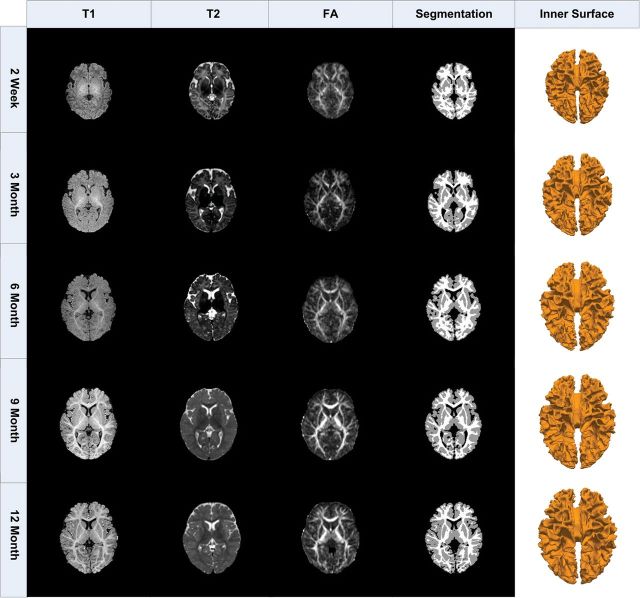
Longitudinal T1, T2, and diffusion-weighted MR images of 10 healthy subjects were acquired at every 3 months from birth to 1 year old, using a 3-T head-only MR scanner. The imaging parameters for T1 images (with 160 axial slices) are as follows: time repetition [TR] = 1900 ms, time echo [TE] = 4.38 ms, flip angle = 7, acquisition matrix = 256 × 192, and voxel resolution = 1 × 1 × 1 mm³; the imaging parameters for T2 images (with 70 axial slices) are as follows: TR = 7380 ms, TE = 119 ms, flip angle = 150, acquisition matrix = 256 × 128, and voxel resolution = 1.25 × 1.25 × 1.95 mm³; and the imaging parameters for diffusion-weighted images (with 60 axial slices) are as follows: TR/TE = 7680/82 ms, matrix size = 128 × 96, 42 noncollinear diffusion gradients, and diffusion weighting b = 1000 s/mm². T2 image is linearly aligned onto the respective T1 image of the same subject and further resampled to 1 × 1 × 1 mm³. Fractional anisotropy (FA) image is reconstructed from the DTI image and then aligned onto the T1 image of the same subject and further resampled to 1 × 1 × 1 mm³. For each set of the aligned T1, T2, and FA images, the skull stripping is first performed to remove noncerebral tissues, and also the cerebellum and brain stem are removed by the in-house–developed tools (as shown at the first, second, and third columns of Fig. 1). Since the delineation of the gray–white interface at 6 months of age is difficult due to low tissue contrast in the T1 and T2 MR images (as shown in Fig. 1), the DTI images, especially the FA images, are further adopted (as in Liu et al. (2007)) to improve the segmentation of white matter (WM), especially for 6-month images. Specifically, the combined T1, T2, and FA image information is used to segment the brain image into gray matter (GM), WM, and cerebrospinal fluid regions (Wang et al. 2011), as shown at the fourth column of Figure 1. The results in Wang et al. (2011), which compare the automatic segmentation results with manual segmentation results, show that the average Dice overlay ratio of cortex is about 0.9 at 6 months, which is similar to the average Dice overlay ratio of 0.9 at 3, 9, 12 months.

Figure 1.

Longitudinal T1, T2, and FA images of the same subject along with its inner cortical surfaces reconstructed from tissue segmentation results.

After topology correction of WM volume (Shattuck and Leahy 2001), the inner cortical surface (i.e., the interface between WM and GM) at different developmental stages can be reconstructed and represented by the triangular meshes composed of a set of vertices and triangles (as shown at the fifth column of Fig. 1). Since the transient subplate zone, which is interposed between the immature cortical plate and WM, may still exist at 2 weeks after birth, the inner cortical surface at 2 weeks is defined as the interface between the cortex plate and WM zone (including WM and transient subplate zone). Due to the effect of partial volume in MR images, the outer surface is relatively hard to be accurately reconstructed, especially in the deep sulcal regions (Fischl et al. 1999; Xu et al. 1999). Thus, the inner cortical surface at birth is used as the initial surface in our model to simulate the cortical development in the first year of life, as detailed below.

Computational Growth Model

In our computational growth model, the cerebral cortex is represented by its inner cortical surface and modeled by a deformable sheet with elastoplasticity property. In this way, the cortical surface can be deformed into dynamic shapes via mechanical forces and can also be restored to its original shape (elasticity) or maintain the dynamic shape permanently (plasticity). Specifically, the development of the cortical surface is modeled by a growth model, which generates the driving force by increasing the “rest” area of the cortical surface (here “rest” indicates the steady status of the cortical surface under no external force). To reduce the simulation error, a guidance model is then introduced to estimate both the growth parameters and the cortical shapes at later developmental stages. Also, a volumetric constraint model is adopted to prevent the cortical surface from deforming into other brain tissues and self-collision. These models are finally incorporated into a time-varying system and further solved by the Newmark scheme (Newmark 1959).

In the following, we will use $S_{t_0}$, $S_{t_1}$, $S_{t_2}$, $S_{t_3}$, and $S_{t_4}$ to denote the inner cortical surfaces reconstructed from the longitudinal images acquired at 2 weeks, 3, 6, 9, and 12 months old of each subject, respectively. We also use $\left\{S_{t_k},k=0,1,2,3,4\right\}$ to represent them. Note that our goal is to develop a growth model that can simulate the continuous cortical development under certain mechanical constraints and also approach all those given cortical surfaces at the known time points.

Deformable Mechanical Model

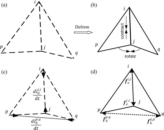
The elastoplasticity model is adopted on each edge of the triangulated inner cortical surface to model the mechanical properties of the developing cortex. For each edge, both “elastic property” and “bending elastic property” are introduced to restore it to its rest shape, and also both plastic property and bending plastic property are introduced to maintain the current shape. An illustration of elastoplasticity property is shown in Figure 2. For each edge element (i, j) and its 2 neighboring triangles Δpij and Δqij, after contracting and bending to a new shape (Fig. 2b) from the original shape (Fig. 2a), the elastic forces are generated on both the edge (i, j) and the virtual edge (p, q) to restore it to its original shape (Fig. 2d), and the rest lengths of the edge (i, j) and the virtual edge (p, q) are adapted to the current lengths by the plastic property (Fig. 2c).

Figure 2.

Illustration of the elastoplasticity properties defined on each edge (i, j), and also the bending properties for the edge (i, j) defined on the virtual edge (p, q). (a) The original shape of edge (i, j) and its 2 neighboring triangles Δpij and Δqij. (b) Edge (i, j) and its 2 neighboring triangles are deformed by, respectively, contracting the edge (i, j) and rotating the 2 triangles. (c) The plasticity of the original lengths $l_0^{i,j}$ and $l_0^{p,q}$ under the current deformation. (d) The elastic forces on the edge (i, j) and the virtual edge (p, q) under the current deformation.

Elastic property and plastic property. At the developmental stage t, the elastic property f_e on each edge (i, j) of the triangulated inner surface is modeled as:

$$f_{\text{e}}^{i,j}\text{(}t\text{)}=K_{\text{e}}\frac{\left(l_0^{i,j}\text{(}t\text{)}-l_{\text{c}}^{i,j}\text{(}t\text{)}\right)}{l_0^{i,j}\text{(}t\text{)}}\frac{\left(x_{\text{c}}^i\text{(}t\text{)}-x_{\text{c}}^j\text{(}t\text{)}\right)}{l_{\text{c}}^{i,j}\text{(}t\text{)}},$$ (1)

where i and j are the 2 ending points on the edge (i, j) as shown in Figure 2a, $l_0^{i,j}\text{(}t\text{)}$is the rest length of the edge (i, j), $l_{\text{c}}^{i,j}\text{(}t\text{)}=\parallel x_{\text{c}}^i\text{(}t\text{)}-x_{\text{c}}^j\text{(}t\text{)}\parallel$ is the current length of the edge (i, j), and $x_{\text{c}}^i\text{(}t\text{)}$ and $x_{\text{c}}^j\text{(}t\text{)}$ are the current coordinates of the vertices i and j, respectively. K_e is the elastic constant that controls the elasticity of the edge (i, j). At the initial stage (t = 0), we have $l_0^{i,j}\text{(}t\text{)}=\parallel x_{\text{c}}^i\text{(}t=0\text{)}-x_{\text{c}}^j\text{(}t=0\text{)}\parallel$, where $x_{\text{c}}^i\text{(}t=0\text{)}$ and $x_{\text{c}}^j\text{(}t=0\text{)}$are the original coordinates of vertices i and j on the inner cortical surface $S_{t_0}$(as described above), respectively. Note that this elastic property will drive each edge to restore to its rest length during the cortical development, as shown in Figure 2d.

At the same time, the plastic property on each edge (i, j) (as shown in Fig. 2c) for maintaining the developed length of the edge is modeled as the adaptation of the rest length $l_{\text{0}}^{i,j}\text{(}t\text{)}$to the deformed length $l_{\text{c}}^{i,j}\text{(}t\text{)}$:

$$\frac{\text{d}{l}_0^{i,j}\text{(}t\text{)}}{\mathrm{d}t}\hspace{0.5em}=\hspace{0.5em}\frac{1}{{\mathrm{\tau }}_{\text{e}}}\left(l_{\text{c}}^{i,j}\text{(}t\text{)}\mathrm{-}{l}_0^{i,j}\text{(}t\text{)}\right),$$ (2)

where τ_e is the time constant for the plasticity (Toro and Burnod 2005).

Bending elastic property and bending plastic property. To model the rigidity of the cortex, the “bending” elastoplasticity property is also defined on each edge (i, j), through a virtual edge (p, $q$) as shown in Figure 2c, where p and q are the vertices that share the same 2 triangles with the edge (i, j). When the angle between the triangles Δpij and Δqij changes, as shown in Figure 2b, the distance between vertices p and q will change accordingly. Thus, similar to equation (1), the bending elastic property f_b on each virtual edge (p, q) is modeled as:

$$f_{\text{b}}^{p,q}\text{(}t\text{)}=K_{\text{b}}\frac{(l_0^{p,q}\text{(}t\text{)}-l_{\text{c}}^{p,q}\text{(}t\text{)})}{l_0^{p,q}\text{(}t\text{)}}\frac{(x_{\text{c}}^p\text{(}t\text{)}-x_{\text{c}}^q\text{(}t\text{)})}{l_{\text{c}}^{p,q}\text{(}t\text{)}},$$ (3)

where $l_0^{p,q}\text{(}t\text{)}$is the rest length of the virtual edge (p, q), $l_{\text{c}}^{p,q}\text{(}t\text{)}=\parallel x_{\text{c}}^p\text{(}t\text{)}-x_{\text{c}}^q\text{(}t\text{)}\parallel$ is the current length of the virtual edge (p, q), and K_b is the elastic constant that controls the bending elasticity of the cortex. At the initial stage (t = 0), we have $l_0^{p,q}\text{(}t\text{)}=\parallel x_{\text{c}}^p\text{(}t=0\text{)}-x_{\text{c}}^q\text{(}t=0\text{)}\parallel$, where $x_{\text{c}}^p\text{(}t=0\text{)}$and $x_{\text{c}}^q\text{(}t=0\text{)}$are the original coordinates of vertices p and q on the cortical surface $S_{t_0}$. Similar to equation (2), the bending plasticity property can be modeled as the adaptation of the rest length $l_0^{p,q}\text{(}t\text{)}$ to the deformed length $l_{\text{c}}^{p,q}\text{(}t\text{)}$:

$$\frac{\text{d}{l}_0^{p,q}\text{(}t\text{)}}{\text{d}t}=\frac{1}{{\mathrm{\tau }}_{\text{b}}}\left(l_{\text{c}}^{p,q}\text{(}t\text{)}\mathrm{-}{l}_0^{p,q}\text{(}t\text{)}\right),$$ (4)

where τ_b is the time constant for the bending plasticity property (Nie et al. 2010).

Cortex Growth Model

Although most neuronal proliferation and migration have been completed before birth (Brown et al. 2002), the volume of the cortex and the size of the brain still keep developing until adolescence because of the further postnatal growth of neuronal dendrites, myelination, and gliogenesis and angiogenesis. Given the later developed surface area of the cortex $A_{S_{t_k}}$, the cortex growth model at time t can be described as the classic logistic growth function (Murray 1993; Toro and Burnod 2005):

$$\frac{\text{d}{A}_{\text{c}}\text{(}t\text{)}}{\text{d}t}=A_{\text{c}}\text{(}t\text{)}·g·\left(\text{1}\mathrm{-}\frac{A_{\text{c}}\text{(}t\text{)}}{A_{S_{t_k}}}\right),t_{k-1}\mathrm{<}t\mathrm{<}{t}_k\mathrm{,}k\mathrm{\ge 1,}$$ (5)

where A_c(t) is the current area of the cortex, and g is known as the Malthusian parameter, and $A_{S_{t_k}}$ is the carrying capacity of the system (Murray 1993), which is defined as the surface area of the later developed cortex $S_{t_k}$. By changing the rest area of each triangle, the rest lengths of the 3 corresponding edges on the triangle will also change accordingly. Thus, the cortical growth will generate a mechanical stress to partially drive the deformation of the cortical surface. At the initial stage, we increase the rest length of each edge element according to the cortical growth function, thus the initial stress could be calculated according to the difference between the current length and rest length of each element.

Guidance Model

Since we have reconstructed cortical surfaces from the later developed stages $\left\{S_{t_k}\text{,}{t}_{k-1}<t<t_k\text{,}k\ge 1\right\}$, these cortical surfaces can be used to guide the cortical development in 2 aspects. First, the parameter in equation (5) can be estimated based on the area of the surface $S_{t_k}$. Second, the simulation to the realistic cortical shape and position can be guided by the shape and position of the cortical surface $S_{t_k}$.

The initial cortical surface $S_{t_0}$is first warped into the space of the target cortical surface $S_{t_k}$ (i.e., the inner cortical surface at 3, 6, 9, and 12 months) by a high-dimensional nonlinear hybrid (volumetric/surface) registration method (Shen and Davatzikos 2002; Liu et al. 2004). Thus, for each vertex i with the position $x_{\text{c}}^i\text{(}t=0\text{)}$ on the initial cortical surface $S_{t_0}$, a rough corresponding vertex ${\left(x_k^i\right)}^{\prime }$ can be found on the target cortical surface $S_{t_k}$. Then, the guidance force $f_{\text{g}}^i$ can be modeled as:

$$f_{\text{g}}^i\text{(}t\text{)}=w({\left(x^i\right)}^{\prime }\text{(}t\text{)}-x_{\text{c}}^i\text{(}t\text{)}),$$ (6)

where w is the weight of the guidance force varying at different cortical regions, and the setting of w will be detailed later. And ${\left(x^i\right)}^{\prime }\text{(}t\text{)}$is the attraction point determined by the later developed cortical surfaces and computed as:

$${\left(x^i\right)}^{\prime }\text{(}t\text{)}=\mathrm{\beta }\text{(}t\text{)}·{\left(x_k^i\right)}^{\prime }+\text{(}1-\mathrm{\beta }\text{(}t\text{))}·{\left(x_{k+1}^i\right)}^{\prime },t_{k-1}<t<t_k,$$ (7)

where ${\left(x_k^i\right)}^{\prime }$ and ${\left(x_{k+1}^i\right)}^{\prime }$ are the correspondences of vertex i at time points k and k + 1 determined by the registration method, respectively; and ${\left(x^i\right)}^{\prime }$ is a linear combination of these 2 correspondences weighted by β(t) as defined below:

$$\mathrm{\beta }\text{(}t\text{)}=\{\begin{array}{cc}\text{1}& \frac{A_{S_{t_k}}-A_{\text{c}}\text{(}t\text{)}}{A_{S_{t_{k+1}}}-A_{S_{t_k}}}>{\mathrm{\beta }}_{\text{th}}\\ \frac{\text{1}}{{\mathrm{\beta }}_{\text{th}}}·\frac{A_{S_{t_k}}-A_{\text{c}}\text{(}t\text{)}}{A_{S_{t_{k+1}}}-A_{S_{t_k}}}& \frac{A_{S_{t_k}}-A_{\text{c}}\text{(}t\text{)}}{A_{S_{t_{k+1}}}-A_{S_{t_k}}}\le {\mathrm{\beta }}_{\text{th}}\end{array},$$ (8)

where β_th is a threshold controlling when the surface $S_{t_{k+1}}$ could be involved into the guidance model. Specifically, when comparing to the area difference between the next 2 target surfaces $\left(A_{S_{t_{k+1}}}-A_{S_{t_k}}\right)$, if the area of the current surface $(A_{\text{c}}\text{(}t\text{))}$ is much smaller than the area of the next target surface $\left(A_{S_{t_k}}\right)$, only the next target surface $S_{t_k}$ will be used to guide the simulation (β(t) = 1). Otherwise, if the current surface area is close to the next target surface area (i.e., $\frac{A_{S_{t_k}}-A_{\text{c}}\text{(}t\text{)}}{A_{S_{t_{k+1}}}-A_{S_{t_k}}}\le {\mathrm{\beta }}_{\text{th}}$), the correspondences on the surface at time k + 1 could also be involved to further guide the simulation. In this way, the corresponding vertex ${\left(x^i\right)}^{\prime }\text{(}t\text{)}$ will smoothly change across different time points.

Since the correspondences in the flat cortical region with low curvature value, such as sulcal wall, determined by the hybrid registration method (Liu et al. 2004) is usually not as accurate as those in the highly bended cortical region with high curvature value, such as gyral crest and sulcal bottom (Li et al. 2009), the weight of the guidance force should be set larger at the highly bended region. Therefore, the weight of the guidance force w is defined as:

$$w=w_1+w_2\text{tanh}(\mathrm{\alpha }·(\text{max}\left(\text{|}{C}_{\text{max}}^i\right|\text{,|}{C}_{\text{min}}^i\text{|})-C_m)),$$ (9)

where w₁, w₂, and α are the weight values, $C_{\text{max}}^i$ and $C_{\text{min}}^i$ are the maximum and minimum principal curvatures of the vertex i, and C_m is a curvature constant. Thus, the guidance model would be smooth during the simulation. Since the force $f_{\text{g}}^i$ is an artificial force that does not truly exist, the weights w₁ and w₂ are both set as small values during the simulation.

Constraints

To prevent the cortical surface from self-collision and deforming into other brain tissues, such as the skull, basal ganglia/thalami, and cerebellum, these tissues and the current deformed cortical surface are first rasterized into a volumetric model (Nie et al. 2010). Then, the deformation of each cortical vertex is prevented from self-collision and deforming into these tissues in this volumetric model.

For each vertex with the current position $x_{\text{c}}^i\text{(}t\text{)}$, when it’s being deformed to a new position $x_{\text{c}}^i\text{(}t\mathrm{+}\Delta t\text{)}$, 2 conditions should be checked: 1) The new position $x_{\text{c}}^i\text{(}t\mathrm{+}\Delta t\text{)}$ cannot be inside of the developing skull or other brain tissue volume as mentioned before and 2) The deformation of the current vertex should not cause its neighboring triangles to intersect with the rasterized surfaces in other neighborhoods. If any of the 2 conditions is violated, a new deformed position ${\tilde{x}}_{\text{c}}^i\text{(}t+\Delta t\text{)}$ is identified as the closest valid position to $x_{\text{c}}^i\text{(}t+\Delta t\text{)}$ on the straight line between $x_{\text{c}}^i\text{(}t\text{)}$ and $x_{\text{c}}^i\text{(}t+\Delta t\text{)}$ as defined below:

$${\tilde{x}}_{\text{c}}^i\text{(}t+\Delta t\text{)}=\mathrm{\theta }{x}_{\mathrm{c}}^i\text{(}t\text{)}+\text{(1}\mathrm{-\theta }\text{)}{x}_{\text{c}}^i\text{(}t+\Delta t\text{),}\mathrm{\theta }\in \text{[0,1]}\text{.}$$ (10)

Note that, after updating the position of a vertex, its neighborhood is re-rasterized.

Model Solver

Since we are applying a mechanical model on the cortex, the dynamics of the cortical surface can be formulated as Newton’s laws:

$$\ddot{\mathbf{x}}={\mathbf{M}}^{-1}F(\mathbf{x},\dot{\mathbf{x}}),$$ (11)

where x, $\dot{\mathbf{x}}$, and $\ddot{\mathbf{x}}$ are the position, velocity, and acceleration of all n vertices on the cortical surface, respectively. M is a 3n × 3n diagonal mass matrix with $\text{diag(}\mathbf{M})=(m_1,m_1,m_1,m_2,m_2,m_2,\dots ,m_n,m_n,m_n),$ where m_i is the mass of the vertex i, calculated as the sum of one thirds of the masses of all one-ring triangles around the vertex i. $F\text{(}\mathbf{x},\dot{\mathbf{x}})$ is the force vector that combines all forces on vertices. For the vertex, i, $F^i\text{(}\mathbf{x},\dot{\mathbf{x}})$is calculated as:

$$F^i\text{(}\mathbf{x}\text{,}\dot{\mathbf{x}}\text{)}={\displaystyle \sum _{j\in N^i}{f}_{\text{e}}^{i,j}\text{(}t\text{)}}+{\displaystyle \sum _{\text{(}p=i\text{)},q}{f}_{\text{b}}^{p,q}\text{(}t\text{)}}+f_{\text{g}}^i\text{(}t\text{),}$$ (12)

where $N^i$ is the one-ring neighboring vertices of the vertex i, and ${\displaystyle {\sum }_{\text{(}p=i\text{)},q}{f}_{\text{b}}^{p,q}\text{(}t\text{)}}$ is the sum of all bending forces involved on the vertex i.

The explicit Newmark scheme (Newmark 1959) is adopted to solve the above dynamic model. Using the position and velocity given in the previous time t, the developed cortical surface at the next time $t+\Delta t$ can be estimated as:

$$\dot{\mathbf{x}}\text{(}t+\Delta t\text{)}=\dot{\mathbf{x}}\text{(}t\text{)}+\Delta t\ddot{\mathbf{x}}\text{(}t\text{),}$$ (13)

$$\mathbf{x}\text{(}t+\Delta t\text{)}=\mathbf{x}\text{(}t\text{)}+\Delta t\dot{\mathbf{x}}\text{(}t+\Delta t\text{)}+\frac{\Delta t^2}{2}\ddot{\mathbf{x}}\text{(}t\text{),}$$ (14)

where $\Delta t$ is the time step. Note that, before estimating the cortical surface at new time, the rest lengths of each edge and each virtual edge are updated by equations (3–5).

Longitudinal Cortical Folding Measurement

With the proposed cortical growth model, we can measure and study the longitudinal changes of the cortical folding. Several quantitative methods for measuring cortical folding have been proposed in the literature. For example, the traditional gyrification index was firstly proposed in Zilles et al. (1988) to measure the cortical folding in a 2D slice and recently extended to the 3D local gyrification by measuring the cortical surface area in a sphere (Schaer et al. 2008; Toro et al. 2008). Meanwhile, curvature-based methods have also been proposed to measure the complexity of the cortical folding especially in the developing brain (Rodriguez-Carranza et al. 2007; Pienaar et al. 2008). Recent comparison on the curvature-based measurement and the gyrification index (Rodriguez-Carranza et al. 2007) also shows that these 2 types of measurements perform similarly on the inner cortical surfaces.

In this paper, 2 curvature-based measures, for example, the curvedness (Koenderink and van Doorn 1992) and sharpness (Pienaar et al. 2008), are adopted to characterize the local change of the cortical folding:

$$c^i\text{(}t\text{)}=\sqrt[\text{2}]{\frac{{\left(C_{\text{max}}^i\text{(}t\text{)}\right)}^2+{\left(C_{\text{min}}^i\text{(}t\text{)}\right)}^2}{\text{2}}},$$ (15)

$$s^i\text{(}t\text{)}={\left(C_{\text{max}}^i\text{(}t\text{)}\mathrm{-}{C}_{\text{min}}^i\text{(}t\text{)}\right)}^2,$$ (16)

where $C_{\text{max}}^i\text{(}t\text{)}$, $C_{\text{min}}^i\text{(}t\text{)}$, $c^i\text{(}t\text{)}$, and $s^i\text{(}t\text{)}$ are the maximum principal curvature, minimum principal curvature, curvedness (Koenderink and van Doorn 1992), and sharpness (Pienaar et al. 2008) of vertex i at time t, respectively. The sharpness $s^i\text{(}t\text{)}$ which emphasizes the difference between 2 principle curvatures is suitable to reveal the large primary folds of the cortex, while the curvedness $c^i\text{(}t\text{)}$ can reveal small bumps and ridges of the cortex (Pienaar et al. 2008).

To measure the changes of curvedness and sharpness in cortical regions, the cortical surface is parcellated into a set of regions of interest (ROIs) by an atlas-based warping method (Shen and Davatzikos 2002), and the relative curvedness and sharpness changes in each ROI are defined, respectively, as:

$${\text{RC}}_{\text{ROI}}\text{(}t\text{)}=\frac{{\displaystyle {\sum }_{i\in \text{ROI}}{c}^i\text{(}t\text{)}}}{{\displaystyle {\sum }_{i\in \text{ROI}}{c}^i\text{(}{t}_0\text{)}}},$$ (17)

$${\text{RS}}_{\text{ROI}}\text{(}t\text{)}=\frac{{\displaystyle {\sum }_{i\in \text{ROI}}{s}^i\text{(}t\text{)}}}{{\displaystyle {\sum }_{i\in \text{ROI}}{s}^i\text{(}{t}_0\text{)}}},$$ (18)

where $t_0$ is the initial time of the cortex development in the cortical growth model, ${\text{RC}}_{\text{ROI}}\text{(}t\text{)}$ and ${\text{RS}}_{\text{ROI}}\text{(}t\text{)}$ are, respectively, the average curvedness and sharpness in one ROI, normalized by their initial values at time t₀ (in order to account for the initial differences among subjects).

Since the curvature decreases with the increase of the cortical surface area even in the case of linear cortical growth, the change of cortical surface area should be normalized in order to measure the cortical folding relatively. Therefore, the normalized relative curvedness and sharpness changes in each ROI can be defined as below:

$${\text{NRC}}_{\text{ROI}}\text{(}{t}_k\text{,}{t}_{k\mathrm{-}\text{1}}\text{)}=\frac{{\displaystyle {\sum }_{i\in \text{ROI}}{c}^i\text{(}{t}_k\text{)}}}{{\displaystyle {\sum }_{i\in \text{ROI}}{c}^i\text{(}{t}_{k-1}\text{)}}}·\sqrt{\frac{A_{\text{ROI}}\text{(}{t}_k\text{)}}{A_{\text{ROI}}\text{(}{t}_{k-1}\text{)}}},$$ (19)

$${\text{NRS}}_{\text{ROI}}\text{(}{t}_k\text{,}{t}_{k\mathrm{-}\text{1}}\text{)}=\frac{{\displaystyle {\sum }_{i\in \text{ROI}}{s}^i\text{(}{t}_k\text{)}}}{{\displaystyle {\sum }_{i\in \text{ROI}}{s}^i\text{(}{t}_{k-1}\text{)}}}·\frac{A_{\text{ROI}}\text{(}{t}_k\text{)}}{A_{\text{ROI}}\text{(}{t}_{k-1}\text{)}},$$ (20)

where $A_{\text{ROI}}\text{(}{t}_k\text{)}$ is the area of ROI at time $t_k$, ${\text{NRC}}_{\text{ROI}}\text{(}{t}_k\text{,}{t}_{k\mathrm{-}\text{1}}\text{)}$ and ${\text{NRS}}_{\text{ROI}}\text{(}{t}_k\text{,}{t}_{k\mathrm{-}\text{1}}\text{)}$ are the normalized change rate of curvedness and sharpness between times $t_k$ and $t_{k\mathrm{-}\text{1}}$, respectively.

Results

The performance of our proposed cortical growth model is evaluated both qualitatively and quantitatively on 10 healthy subjects (each with longitudinal images collected at 2 weeks, 3, 6, 9, and 12 months old) and is further compared with a high-dimensional nonlinear hybrid (volumetric/surface) registration algorithm (Liu et al. 2004). In our method, we use the inner cortical surfaces at 6 and 12 months old to help build our cortical growth model and then use the inner cortical surfaces reconstructed at 3 and 9 months old as the ground truth to evaluate the prediction power of our model. Note that, after building our cortical growth model, given any time in the first year, we can immediately estimate its corresponding cortical surface, that is, at 3 or 9 months old. Similarly, for the hybrid registration algorithm, we can also build its respective brain growth model by registering the 2-week-old image to the 6-month-old image and then to the 12-month-old image. In this case, the brain image at 3 or 9 months old can be estimated by resampling the estimated deformation fields by constraining the respective cortical surface area to be the same as that in the ground truth 3- or 9-month-old cortical surface. It is worth noting that this cortical surface area information is not used in our model when estimating cortical surfaces at 3 and 9 months.

In all experiments, the same parameters are used, that is, K_e = 0.1, τ_e = 50, K_b = 0.1, τ_b = 50, g = 0.01, w₁ = 0.006, w₂ = 0.004, β_th = 2.0, C_m = 0.7, α = 3.0, and Δt = 0.05. We use 240 iterations in building the cortical growth model for the first year, thus the real-world unit for time in our implementation is month (each with 20 iterations). Our model takes about 4 h to build the cortical growth model for each subject on a PC with Inter Xeon 2.26 Ghz CPU and 4 GB memory.

Visual Inspection of the Accuracy

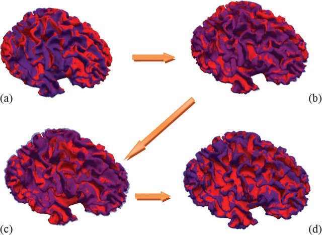
Figure 3 gives a comparison between the cortical surfaces predicted by our model (red color) and the ground truth (light blue color) reconstructed at 3, 6, 9, and 12 months old. Note that the ground truth surfaces are set to be transparent for better visual inspection. With the cortical surface guidance at 6 and 12 months old, our predicted cortical surfaces have the similar shapes and positions to the ground truth at the respective time points, as shown in Figure 3b,d, respectively. Also, at other time points without any guidance, our predicted cortical surfaces still have the similar shapes and positions to the ground truth, as shown in Figure 3a,c.

Figure 3.

Comparison between the cortical surfaces predicted by our model (red colors) and the ground truth cortical surfaces (light blue colors) at 3, 6, 9, and 12 months old, as shown from (a) to (d), respectively.

Quantitative Evaluation of the Accuracy

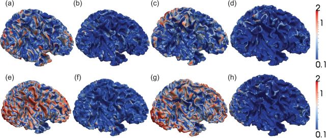
To quantitatively evaluate our model and further compare its performance with the hybrid registration algorithm (Liu et al. 2004), we measure the surface distance error between the predicted surface and the ground truth surface at each time point (from 3 to 12 months old) on all 10 subjects. Note that the surface distance is symmetrically computed between the 2 surfaces under comparison. Figure 4 shows a comparison of surface distance errors between our method and the hybrid registration method on one subject at 4 different time points. It can be observed that the surface distance errors between the cortical surfaces predicted by our model and the ground truth cortical surfaces at 3, 6, 9, and 12 months old, as shown in Figure 4a–d, respectively, are much smaller than the surface distance errors between the cortical surfaces predicted by the hybrid registration algorithm and the ground truth cortical surfaces at 3, 6, 9, and 12 months old, as shown in Figure 4e–h, respectively.

Figure 4.

Comparison of surface distances errors (mm) of one subject at 4 time points from 3 to 12 months old. (a–d) are the surface distance errors between the cortical surfaces predicted by our model and the ground truth cortical surfaces at 3, 6, 9, and 12 months old, respectively. (e–h) are the surface distance errors between the cortical surfaces predicted by the hybrid registration algorithm and the ground truth cortical surfaces at 3, 6, 9, and 12 months old, respectively. The color bars are shown on the right.

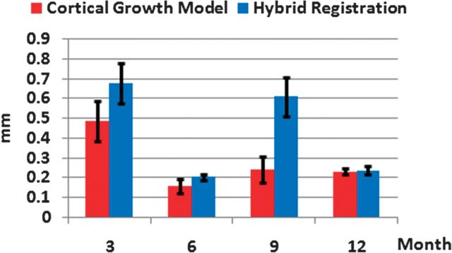
The comparison of the averages and standard deviations of surface distance errors of 10 subjects between our model and the hybrid registration algorithm at 4 time points (from 3 to 12 months old) is shown in Figure 5. With the surface guidance at 6 and 12 months old, the average surface distance for all subjects is smaller than 0.25 mm by both our model and the hybrid registration algorithm, which also use the 6- and 12-month-old images and surfaces to guide the registration. For the time points without surface guidance such as at 3 and 9 months old, the average surface distances for all subjects are 0.48 ± 0.10 and 0.24 ± 0.06 mm by our model, respectively, and 0.68 ± 0.10 and 0.61 ± 0.10 mm by the hybrid registration algorithm, respectively. Considering the small brain size in the first year of life, this improvement is significant for early brain development study. This experiment demonstrates that our proposed model can predict more accurate cortical surfaces with use of the mechanical models compared with the hybrid registration algorithm that considers only the image- and surface-derived information in the registration.

Figure 5.

Comparison of the averages and standard deviations of surface distance errors of 10 subjects between our model (red bars) and the hybrid registration algorithm (blue bars) at 4 time points from 3 to 12 months old.

Smoothness and Consistency of Cortex Growth on Vertices

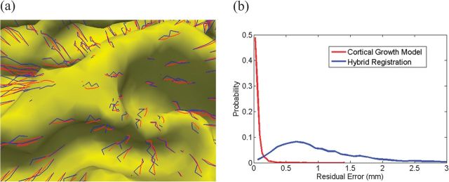
We further visually evaluate the smoothness and consistency of the longitudinal cortical surfaces predicted by our model, by comparison with those by the hybrid registration algorithm. As shown in Figure 6a, the trajectories of vertex growth (red curves) predicted by our model along 5 time points (from 2 weeks to 12 months) are much smoother even in the flat cortical surface regions compared with those (blue curves) produced by the hybrid registration algorithm that registers the 2-week-old image/surface to images/surfaces at other 4 time points. To quantitatively compare the performance, we first perform the linear regression on the trajectory of each vertex and then show the histogram of the residual errors in the whole cortical surface. As shown in Figure 6b, our method gives smaller residual errors than the hybrid registration method.

Figure 6.

Comparison of the smoothness of vertex growth by our cortical growth model (red colors) and the hybrid registration algorithm (blue colors). (a) Trajectories of vertex growth by 2 methods. (b) The distribution of residual errors after performing linear regression on each trajectory by 2 methods.

We also measure the smoothness and consistency between neighboring vertices. The relative local area ${\text{RA}}^i\text{(}t\text{)}$ and relative edge length ${\text{RL}}^i\text{(}t\text{)}$ of each vertex i at time t are defined as:

$${\text{RA}}^i\text{(}t\text{)}=\frac{{\displaystyle {\sum }_{j\in T^i}{A}_{\text{tri}}^j\text{(}t\text{)}}}{{\displaystyle {\sum }_{j\in T^i}{A}_{\text{tri}}^j\text{(}{t}_0\text{)}}},$$ (21)

$${\text{RL}}^i\text{(}t\text{)}=\frac{{\displaystyle {\sum }_{j\in N^i}{l}_{\text{c}}^{i,j}\text{(}t\text{)}}}{{\displaystyle {\sum }_{j\in N^i}{l}_{\text{c}}^{i,j}\text{(}{t}_0\text{)}}},$$ (22)

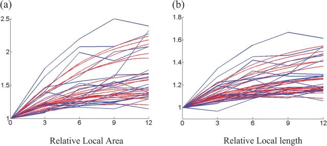
where Tⁱ is the one-ring neighboring triangles of vertex i, Nⁱ is the one-ring neighboring vertices of vertex i, and $A_{\text{tri}}^j\text{(}t\text{)}$ is the area of triangle j at time t. Thus, ${\text{RA}}^i\text{(}t\text{)}$ is the sum of triangular areas around vertex i normalized by the initial area, and ${\text{RL}}^i\text{(}t\text{)}$ is the sum of vertex distances between vertex i and its neighboring vertices normalized by the initial distance. We compute ${\text{RA}}^i\text{(}t\text{)}$ and ${\text{RL}}^i\text{(}t\text{)}$, respectively, from the cortical surfaces predicted by our model from 2 weeks to 12 months and also by the hybrid registration algorithm that registers the 2-week-old image/surface to images/surfaces at other 4 time points. In Figure 7a,b, the respective results by the 2 methods on 20 randomly selected vertices are shown, with red for our model and blue for the hybrid registration. Compared with the hybrid registration, our method can predict much smoother growth for the relative local area and the relative edge length from 2 weeks to 12 months.

Figure 7.

The growth of the relative local area (a) and the relative edge length (b) on 20 randomly selected vertices from 2 weeks to 12 months, by our model (red) and the hybrid registration method (blue).

Smoothness and Consistency of Cortex Growth on ROIs

To further compare the smoothness and consistency in larger cortical regions, an atlas with 90 labeled ROIs (Tzourio-Mazoyer et al. 2002) is warped onto the subject image space to label the subject cortical surface into a set of ROIs. For each ROI, the relative cortical area ${\text{RA}}_{\text{ROI}}\text{(}t\text{)}$ and the relative edge length ${\text{RL}}_{\text{ROI}}\text{(}t\text{)}$ are respectively defined as:

$${\text{RA}}_{\text{ROI}}\text{(}t\text{)}=\frac{{\displaystyle {\sum }_{j\in T_{\text{ROI}}}{A}_{\text{tri}}^j\text{(}t\text{)}}}{{\displaystyle {\sum }_{j\in T_{\text{ROI}}}{A}_{\text{tri}}^j\text{(}{t}_0\text{)}}},$$ (23)

$${\text{RL}}_{\text{ROI}}\text{(}t\text{)}=\frac{{\displaystyle {\sum }_{j\in L_{\text{ROI}}}{l}_{\text{edge}}^j\text{(}t\text{)}}}{{\displaystyle {\sum }_{j\in L_{\text{ROI}}}{l}_{\text{edge}}^j\text{(}{t}_0\text{)}}},$$ (24)

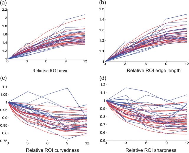
where T_ROI and L_ROI are the set of triangles and edges in the ROI, respectively, $l_{\text{edge}}^j\text{(}t\text{)}$ is the length of edge j at time t, ${\text{RA}}_{\text{ROI}}\text{(}t\text{)}$ is the area of the ROI normalized by its initial area, and ${\text{RL}}_{\text{ROI}}\text{(}t\text{)}$ is the sum of all edge lengths in the ROI normalized by its initial value. In Figure 8a,b, the results on 20 randomly selected cortical ROIs (from 90 ROIs) are given for our method (red) and the hybrid registration (blue). As we can see, our model shows much more consistent growth results.

Figure 8.

The changes of cortical features on 20 cortical ROIs from 2 weeks to 12 months. (a) Relative ROI area. (b) Relative ROI edge length. (c) Relative ROI curvedness. (d) Relative ROI sharpness. Red and blue curves represent the results by our model and the hybrid registration method, respectively.

To quantify the smoothness and consistency of cortical folding features, the relative curvedness ${\text{RC}}_{\text{ROI}}\text{(}t\text{)}$ and the relative sharpness ${\text{RS}}_{\text{ROI}}\text{(}t\text{)}$ are also measured from the cortical surfaces predicted by our method (red) and the hybrid registration (blue) on 20 ROIs in Figure 8c,d. As we can see, both curvedness ${\text{RC}}_{\text{ROI}}\text{(}t\text{)}$ and sharpness ${\text{RS}}_{\text{ROI}}\text{(}t\text{)}$ are decreasing smoothly in most ROIs with the growth of the brain according to our model, while they are bumpy by the hybrid registration method.

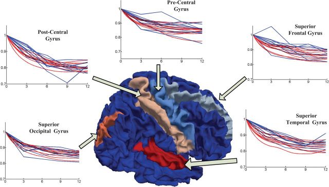
We also show in Figure 9 the changes of the relative curvedness on 5 major gyri, including the precentral gyrus, postcentral gyrus, superior temporal gyrus, superior occipital gyrus, and superior frontal gyrus, on the 10 subjects by the 2 methods. Although both methods show the consistent decreasing trend of curvedness on all 5 gyral ROIs, the results from our method show much smoother results for all subjects.

Figure 9.

The changes of average relative curvedness on 5 major gyral ROIs of the 10 subjects by our cortical growth model (red curves) and the hybrid registration method (blue curves), from 2 weeks to 12 months.

Cortical Folding Pattern from 2 Weeks to 12 Months

Since the above results have already demonstrated the accuracy, smoothness, and consistency of our proposed method, we apply it to measure the cortical folding changes from 2 weeks to 12 months. Note that we use the inner cortical surfaces reconstructed from images at all 5 time points to help build our cortical growth model in this experiment.

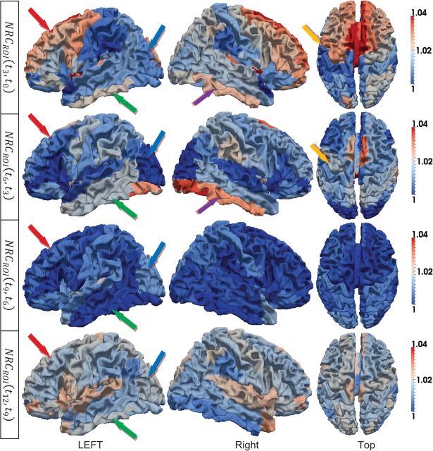
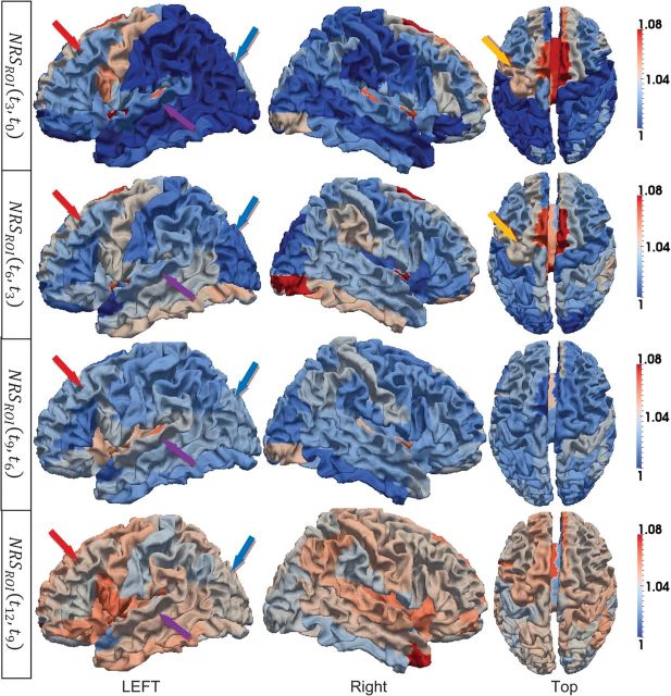
Since the primary and secondary folding structures have been developed before birth, the simple increasing of the cortical surface area will reduce the averages of curvedness and sharpness from 2 weeks to 12 months as shown in Figure 8c,d, respectively. The normalized changes of curvedness ${\text{NRC}}_{\text{ROI}}\text{(}{t}_k\text{,}{t}_{k\mathrm{-}1}\text{)}$ and sharpness ${\text{NRS}}_{\text{ROI}}\text{(}{t}_k\text{,}{t}_{k\mathrm{-}1}\text{)}$ from 2 weeks to 12 months on the 10 subjects are illustrated in Figures 10 and 11, respectively.

Figure 10.

ROI-based average curvedness changes on the 10 subjects from 2 weeks to 12 months old. The changes from 2 weeks to 3 months, 3–6 months, 6–9 months, and 9–12 months are shown from the first to the fourth row, respectively. The color bars are given on the right. In each row, both side views and top view are displayed.

Figure 11.

ROI-based average sharpness changes on the 10 subjects from 2 weeks to 12 months old. The changes from 2 weeks to 3 months, 3–6 months, 6–9 months, and 9–12 months are shown from the first to the fourth row, respectively. The color bars are given on the right. In each row, both side views and top view are displayed.

As we can see, though the normalized changes of curvedness and sharpness are continuously increasing during the first year, the cortical folding shows different changing patterns in different lobes. For example, the frontal lobe shows rapidly increasing cortical folding during this period, which corresponds to high-level function development in this lobe, as indicated by red arrows in both Figures 10 and 11. While in the occipital and parietal lobes, the cortical folding is increasing relatively slower as indicated by blue arrows in both Figures 10 and 11. And in the temporal lobe, the folding changes are even more complex on the 3 major gyri. Specifically, in the first 3 months, the curvedness of the inferior temporal gyrus increases faster than the middle temporal gyrus and increases slower after 3 months as indicated by green arrows in Figure 10. On the contrary, the folding changing speed of the superior temporal gyrus continues to increase during the first year as indicated by purple arrows in Figure 11.

The cortical folding also shows different patterns in different time periods. For example, in the frontal lobe, the curvedness and sharpness increase fast in the first 3 months and then slow down from 3 to 9 months, as indicated by red arrows in both Figures 10 and 11. The average sharpness in both pre- and postcentral gyri increases consistently during the first year after birth, although the precentral gyrus shows stronger increasing folding patterns from 2 weeks to 6 months, as indicated by orange arrows in Figures 10 and 11.

Certain hemispheric asymmetry could also be observed in Figures 10 and 11. For example, the left hemisphere shows faster increase of sharpness on precentral gyri as indicated by light orange arrows in Figure 11 from 2 weeks to 6 months, while the right hemisphere shows faster increase of curvedness on inferior temporal gyrus as indicated by purple arrows in Figure 10 from 2 weeks to 6 months.

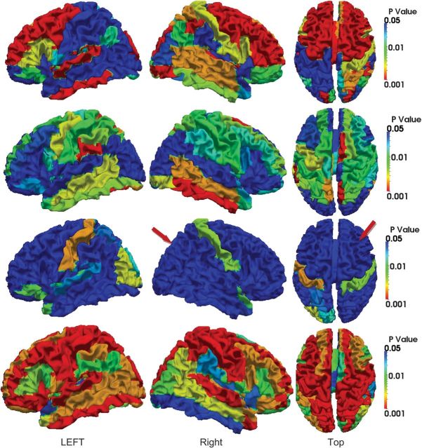
Since the number of subjects (only 10 subjects in our results) is limited in our experiment, the statistical significance of curvedness and sharpness changes is measured by the P value in nonparametric permutation tests (Nichols and Holmes 2002) on each ROI with the null hypothesis that the mean values of and are greater than 1, and the results are shown in Figures 12 and 13, respectively. These results show similar pattern as in Figures 10 and 11. However, it is very interesting that during the period from 6 to 9 months, most cortical ROIs show no significant increase of curvedness, especially in the right hemisphere as indicated by red arrows in Figure 12. And during the first 3 months, the increase of sharpness in the most areas of occipital and temporal lobe is not significant as indicated by red arrows in Figure 13.

Figure 12.

P values of ROI-based curvedness changes on the 10 subjects, from 2 weeks to 12 months old. The results from 2 weeks to 3 months, 3–6 months, 6–9 months, and 9–12 months are shown from the first to the fourth row, respectively. The color bars are given on the right. In each row, both side views and top view are displayed.

Figure 13.

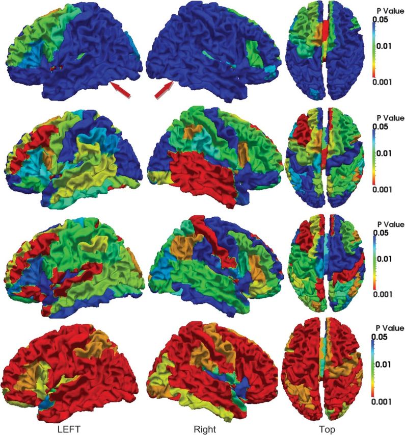
P values of ROI-based sharpness changes on the 10 subjects, from 2 weeks to 12 months old. The results from 2 weeks to 3 months, 3–6 months, 6–9 months, and 9–12 months are shown from the first to the fourth row, respectively. The color bars are given on the right. In each row, both side views and top view are displayed.

Discussion and Conclusion

Due to lack of information in the smooth and flat cortical regions, traditional deformable registration method is limited to correctly estimate tissue deforation over time in these regions as shown in our result. Even though longitudinal regulations could be added to partially compensate for this lack of information and also generate longitudinal smooth and consistent deformation to some degree, our model that takes into account the physical properties of the growing brain is expected to perform better than the registration method that simply assumes smoothly varying deformations.

By coupling longitudinal image analysis with physical models of the cortical growth, we have presented a computational growth model for cortical development in the first year of life. Experimental results show its good performance in predicting cortical surface development at unknown time points in the first year, with the help of mechanical modeling. These results also demonstrate that the features of cortical surfaces, such as curvedness and sharpness, are much more smoothly and consistently estimated by our proposed model than those by the hybrid registration method. Certain interesting developmental patterns of cortical folding in the first year of life are also reported in our results: 1) the curvedness and sharpness decrease from 2 weeks to 12 months; 2) the frontal lobe shows rapidly increasing cortical folding during this period, while the cortical folding increases relatively slower in the occipital and parietal lobes; 3) during the first 3 months, the curvedness of the inferior temporal gyrus increases faster than the middle temporal gyrus and increases slower after 3 months, whereas the folding changing speed of the superior temporal gyrus continues to increase during the first year, and 4) the cortical folding of the frontal lobe also seems to develop fastest during the first 3 months and after that slows down. Due to the complex neurobiological processes involved in the cortex development during this stage, such as WM myelination, synapse development, and neuron dendritic projection, our growth model is not complex enough to cover all possible developing factors currently. For example, we currently use the spatially uniform growth function in our growth model since we do not know the spatial distribution of growth rate. And since the axon tension could also have effect on cortical folding (Van Essen 1997), it is possible to incorporate the axon tension into our model by making use of DTI data sets. In the future study, a more advanced and sophisticated model further involving WM and functional development will be developed to simulate this procedure.

Since only the inner cortical surface is adopted in our method to represent the geometry of the cortex currently, certain important features of the cortex could not be easily measured from our results, such as the cortical thickness (Fischl and Dale 2000) and gyrification index (Zilles et al. 1988), which are usually defined on the outer cortical surface. However, our current model can still provide abundant information regarding the cortex development from different levels and aspects. In the future, we will carry out more experiments and measurements to further evaluate our cortical growth model and apply it to a large early brain development study.

Funding

National Institutes of Health (EB006733, EB008374, EB009634, MH088520, NS055754, HD053000, and MH070890).

References

- Awate SP, Yushkevich PA, Song Z, Licht DJ, Gee JC. Cerebral cortical folding analysis with multivariate modeling and testing: studies on gender differences and neonatal development. Neuroimage. 2010;53:450–459. doi: 10.1016/j.neuroimage.2010.06.072. [DOI] [PMC free article] [PubMed] [Google Scholar]
- Brown M, Keynes R, Lumsden A. The developing brain. Oxford: Oxford University Press; 2002. [Google Scholar]
- Dubois J, Benders M, Borradori-Tolsa C, Cachia A, Lazeyras F, Ha-Vinh Leuchter R, Sizonenko SV, Warfield SK, Mangin JF, Huppi PS. Primary cortical folding in the human newborn: an early marker of later functional development. Brain. 2008;131:2028–2041. doi: 10.1093/brain/awn137. [DOI] [PMC free article] [PubMed] [Google Scholar]
- Fischl B, Dale AM. Measuring the thickness of the human cerebral cortex from magnetic resonance images. Proc Natl Acad Sci U S A. 2000;97:11050–11055. doi: 10.1073/pnas.200033797. [DOI] [PMC free article] [PubMed] [Google Scholar]
- Fischl B, Sereno MI, Dale AM. Cortical surface-based analysis. II: Inflation, flattening, and a surface-based coordinate system. Neuroimage. 1999;9:195–207. doi: 10.1006/nimg.1998.0396. [DOI] [PubMed] [Google Scholar]
- Geng G, Johnston LA, Yan E, Britto JM, Smith DW, Walker DW, Egan GF. Biomechanisms for modelling cerebral cortical folding. Med Image Anal. 2009;13:920–930. doi: 10.1016/j.media.2008.12.005. [DOI] [PubMed] [Google Scholar]
- Grinspun E, Hirani AN, Desbrun M, Schr P. Proceedings of the 2003 ACM SIGGRAPH/Eurographics symposium on Computer animation. San Diego (CA): Eurographics Association; 2003. Discrete shells; pp. 62–67. [Google Scholar]
- Kaukola T, Kapellou O, Laroche S, Counsell SJ, Dyet LE, Allsop JM, Edwards AD. Severity of perinatal illness and cerebral cortical growth in preterm infants. Acta Paediatr. 2009;98:990–995. doi: 10.1111/j.1651-2227.2009.01268.x. [DOI] [PubMed] [Google Scholar]
- Koenderink JJ, van Doorn AJ. Surface shape and curvature scales. Image Vis Comput. 1992;10:557–564. [Google Scholar]
- Li G, Guo L, Nie J, Liu T. Automatic cortical sulcal parcellation based on surface principal direction flow field tracking. Neuroimage. 2009;46:923–937. doi: 10.1016/j.neuroimage.2009.03.039. [DOI] [PMC free article] [PubMed] [Google Scholar]
- Liu T, Li H, Wong K, Tarokh A, Guo L, Wong S. Brain tissue segmentation based on DTI data. Neuroimage. 2007;38(1):114–123. doi: 10.1016/j.neuroimage.2007.07.002. [DOI] [PMC free article] [PubMed] [Google Scholar]
- Liu T, Shen D, Davatzikos C. Deformable registration of cortical structures via hybrid volumetric and surface warping. Neuroimage. 2004;22:1790–1801. doi: 10.1016/j.neuroimage.2004.04.020. [DOI] [PubMed] [Google Scholar]
- Murray JD. Mathematical biology. 2nd ed. Heidelberg (Germany): Springer-Verlag; 1993. [Google Scholar]
- Newmark NM. A method of computation for structural dynamics. J Eng Mech. 1959;85:67–94. [Google Scholar]
- Nichols TE, Holmes AP. Nonparametric permutation tests for functional neuroimaging: a primer with examples. Hum Brain Mapp. 2002;15:1–25. doi: 10.1002/hbm.1058. [DOI] [PMC free article] [PubMed] [Google Scholar]
- Nie J, Guo L, Li G, Faraco C, Stephen Miller L, Liu T. A computational model of cerebral cortex folding. J Theor Biol. 2010;264:467–478. doi: 10.1016/j.jtbi.2010.02.002. [DOI] [PMC free article] [PubMed] [Google Scholar]
- Pienaar R, Fischl B, Caviness V, Makris N, Grant PE. A methodology for analyzing curvature in the developing brain from preterm to adult. Int J Imaging Syst Technol. 2008;18:42–68. doi: 10.1002/ima.v18:1. [DOI] [PMC free article] [PubMed] [Google Scholar]
- Rodriguez-Carranza CE, Mukherjee P, Vigneron D, Barkovich J, Studholme C. Comparing 3D gyrification index and area-independent curvature-based measures in quantifying neonatal brain folding. Proc. SPIE. 2007;6512:65120N. [Google Scholar]
- Schaer M, Cuadra MB, Tamarit L, Lazeyras F, Eliez S, Thiran JP. A surface-based approach to quantify local cortical gyrification. IEEE Trans Med Imaging. 2008;27:161–170. doi: 10.1109/TMI.2007.903576. [DOI] [PubMed] [Google Scholar]
- Schumann CM, Bloss CS, Barnes CC, Wideman GM, Carper RA, Akshoomoff N, Pierce K, Hagler D, Schork N, Lord C, et al. Longitudinal magnetic resonance imaging study of cortical development through early childhood in autism. J Neurosci. 2010;30:4419–4427. doi: 10.1523/JNEUROSCI.5714-09.2010. [DOI] [PMC free article] [PubMed] [Google Scholar]
- Shattuck DW, Leahy RM. Automated graph-based analysis and correction of cortical volume topology. IEEE Trans Med Imaging. 2001;20:1167–1177. doi: 10.1109/42.963819. [DOI] [PubMed] [Google Scholar]
- Shaw P, Eckstrand K, Sharp W, Blumenthal J, Lerch JP, Greenstein D, Clasen L, Evans A, Giedd J, Rapoport JL. Attention-deficit/hyperactivity disorder is characterized by a delay in cortical maturation. Proc Natl Acad Sci U S A. 2007;104:19649–19654. doi: 10.1073/pnas.0707741104. [DOI] [PMC free article] [PubMed] [Google Scholar]
- Shen D, Davatzikos C. HAMMER: hierarchical attribute matching mechanism for elastic registration. IEEE Trans Med Imaging. 2002;21:1421–1439. doi: 10.1109/TMI.2002.803111. [DOI] [PubMed] [Google Scholar]
- Shen EY, Wu KH, Lin MF, Chen CY. Study of brain growth in children—a new approach to volume measurements using MRI-reconstructed 3D neuroimaging. Childs Nerv Syst. 2010;26:1619–1623. doi: 10.1007/s00381-010-1280-1. [DOI] [PubMed] [Google Scholar]
- Talairach J, Tournoux P. Co-planar stereotaxic atlas of the human brain. Stuttgart (Germany): Thieme; 1988. [Google Scholar]
- Toro R, Burnod Y. A morphogenetic model for the development of cortical convolutions. Cereb Cortex. 2005;15:1900–1913. doi: 10.1093/cercor/bhi068. [DOI] [PubMed] [Google Scholar]
- Toro R, Perron M, Pike B, Richer L, Veillette S, Pausova Z, Paus T. Brain size and folding of the human cerebral cortex. Cereb Cortex. 2008;18:2352–2357. doi: 10.1093/cercor/bhm261. [DOI] [PubMed] [Google Scholar]
- Tzourio-Mazoyer N, Landeau B, Papathanassiou D, Crivello F, Etard O, Delcroix N, Mazoyer B, Joliot M. Automated anatomical labeling of activations in SPM using a macroscopic anatomical parcellation of the MNI MRI single-subject brain. Neuroimage. 2002;15:273–289. doi: 10.1006/nimg.2001.0978. [DOI] [PubMed] [Google Scholar]
- Van Essen DC. A tension-based theory of morphogenesis and compact wiring in the central nervous system. Nature. 1997;385:313–318. doi: 10.1038/385313a0. [DOI] [PubMed] [Google Scholar]
- Van Essen DC, Maunsell JH. Two-dimensional maps of the cerebral cortex. J Comp Neurol. 1980;191:255–281. doi: 10.1002/cne.901910208. [DOI] [PubMed] [Google Scholar]
- Vercauteren T, Pennec X, Perchant A, Ayache N. Diffeomorphic demons: efficient non-parametric image registration. Neuroimage. 2009;45:S61–S72. doi: 10.1016/j.neuroimage.2008.10.040. [DOI] [PubMed] [Google Scholar]
- Wang L, Shi F, Yap P-T, Gilmore JH, Lin W, Shen D. Accurate and Consistent 4D Segmentation of Serial Infant Brain MR Images. LNCS. 2011;7012:93–101. [Google Scholar]
- Woods RP, Grafton ST, Watson JD, Sicotte NL, Mazziotta JC. Automated image registration: II. Intersubject validation of linear and nonlinear models. J Comput Assist Tomogr. 1998;22:153–165. doi: 10.1097/00004728-199801000-00028. [DOI] [PubMed] [Google Scholar]
- Xu C, Pham DL, Rettmann ME, Yu DN, Prince JL. Reconstruction of the human cerebral cortex from magnetic resonance images. IEEE Trans Med Imaging. 1999;18:467–480. doi: 10.1109/42.781013. [DOI] [PubMed] [Google Scholar]
- Zilles K, Armstrong E, Schleicher A, Kretschmann HJ. The human pattern of gyrification in the cerebral cortex. Anat Embryol (Berl) 1988;179:173–179. doi: 10.1007/BF00304699. [DOI] [PubMed] [Google Scholar]