Abstract
Models built using mean data can represent only a very small percentage, or none, of the population being modeled, and produce different activity than any member of it. Overcoming this ‘averaging’ pitfall requires measuring, in single individuals in single experiments, all of the system’s defining characteristics. We have developed protocols that allow all the parameters in the curves used in typical Hill-type models (passive and active force-length, series elasticity, force-activation, force-velocity) to be determined from experiments on individual stick insect muscles (Blümel et al. 2011a). A requirement for means to not well represent the population is that the population shows large variation in its defining characteristics. We therefore used these protocols to measure extensor muscle defining parameters in multiple animals. Across-animal variability in these parameters can be very large, ranging from 1.3 to 17-fold. This large variation is consistent with earlier data in which extensor muscle responses to identical motor neuron driving showed large animal-to-animal variability (Hooper et al. 2006), and suggests accurate modeling of extensor muscles requires modeling individual-by-individual. These complete characterizations of individual muscles also allowed us to test for parameter correlations. Two parameter pairs significantly co-varied, suggesting that a simpler model could as well reproduce muscle response.
Keywords: Carausius morosus, stick insect, invertebrate
1 Introduction
In many systems activity arises emergently from the interaction of multiple fundamental properties. For instance, muscle activity results from passive muscle responses to length changes, the force-length curve, and the force-velocity curve, with the latter two needing to be defined at all muscle activations. System properties are typically defined by equations with multiple parameters (e.g., the spring constant in a passive muscle equation) which can show large across-animal variation. In such systems individual animals having mean values for all these parameters can represent only a very small percentage, or none, of the population, and models built from such means can fail to reproduce the activity of any member of the population (Golowasch et al. 2002; Schulz et al. 2006; see Introduction of Blümel et al. 2011a for detailed examples). In such cases, accurate modeling either requires 1) modeling on an individual-by-individual basis, or 2) having sufficient understanding of how the properties interact to choose parameter values that result in the desired activity (in most cases, the mean activity of the population).
A requirement for ‘averaging’ approaches to fail is that the defining properties of the system show large inter-individual variation. Such variation alone does not necessarily result in the population showing great variation in activity, as counterbalancing variation can allow individuals that differ on the fundamental level nonetheless to produce similar or identical activity. Large variation in activity in response to identical input, alternatively, does likely indicate variation in fundamental make-up. Both stick insect (Carausius morosus) extensor (Hooper et al. 2006) and lobster (Panulirus interruptus) (Thuma et al. 2003) muscle contractions show large inter-individual variation when the muscles (within each species) receive identical neural driving. These observations thus suggest that these muscles may show large across-individual variation in fundamental characteristic make-up.
Muscle fundamental characteristics (passive and active force-length, series elasticity, force-activation and force-velocity relationships) are typically described by Hill-type equations (Hannaford and Winters 1990; Hill 1938, 1950; Winters 1990; Zahalak 1990; Zajac and Winters 1990). Prior work in stick insect has shown that the equations describing these characteristics have the same form across animals (Guschlbauer et al. 2007). The variation in muscle activity noted above thus presumably arises from inter-animal variation in the values of the parameters in these equations. Stick insect extensor muscles thus likely provide a good venue in which to investigate the possible difficulties noted earlier of mean-based modeling approaches.
A difficulty with fulfilling this goal, however, is that, as is typical of muscle (and neuron) characterizations, in prior work the values of only one or at most a few parameters were measured in experiments on any single extensor muscle. Although standard deviations, and sometimes even individual data points, were typically provided in such work, examining across-animal variation has generally not been its motivating purpose. Furthermore, since in this approach all parameters were never measured in any single muscle, these data cannot be used to test for co-variation between parameters, or to test the extent that modeling using individual muscle specific parameter values improves muscle model performance (Blümel et al. 2011b).
We have developed techniques for measuring all Hill-type parameters in experiments on single extensor muscles of the stick insect (Blümel et al. 2011a). This approach allows us to directly measure both how much variability is present across extensor muscles and whether any of the parameters co-vary. We report here that there is substantial (1.3 to 17-fold) parameter variation across muscles, suggesting that individual-by-individual modeling of stick insect may substantially improve model performance. Two of the parameter pairs co-vary. One of these pairs is of parameters in equations that model different muscle characteristics, suggesting a connection between these characteristics that would allow a reduction of standard Hill models. The failure of this co-variation to have been described before underscores the potential advantages of individual-by-individual descriptions of muscle properties.
2 Materials and Methods
2.1 Muscle experimental procedures
Ten extensor muscles were examined in this work. All experimental and parameter measurement procedures were identical to those described in Blümel et al. 2011a.
2.2 Correlation analysis
The Hill-type model used here has ten measured parameters. Our ability to measure all of these parameters in single muscles allowed us not only to describe each muscle individually, but to test for correlations among the parameters across muscles. Because the individual parameters across the ten muscles were sometimes not normally distributed, it was necessary to use non-parametric correlation tests. A Spearman rank correlation was therefore used with a nominal α level of 0.05, adjusted to 0.00114 () to compensate for 10 multiple comparisons being made from a single data set, which corresponds to R values ≥0.903 (Ramsey 1989). Of the two parameters that were not normally distributed (k3 and vmax neg), in each case the non-normality was due to the presence of a single outlier (the ‘31.2’ and ‘3.99’ values, respectively, see Table 1). Removing these outliers and repeating the correlation analysis with simple linear fits (with the above multiple comparison compensation being performed) identified the same correlations, and failed to reveal any additional ones.
Table 1.
Variation of extensor muscle Hill-type parameters across the 10 animals used here. Parameter values have been expressed in the units most convenient for presentation.
| Animal |
k1 (µN) |
k2 (mm−1) |
k3 (N/mm2) |
Fmax (mN) |
A | B |
curvω (mm0.5) |
vmax (act=1) (mm/s) |
vmax neg (mm/s) |
cneg |
|---|---|---|---|---|---|---|---|---|---|---|
| A | 1.76 | 4.73 | 12.1 | 189 | 10.8 | 0.23 | 4.23 | 6.27 | 1.07 | −1.42 |
| B | 4.87 | 4.11 | 11.6 | 197 | 6.6 | 0.32 | 3.23 | 6.02 | 0.60 | −1.26 |
| C | 0.78 | 5.48 | 13.6 | 139 | 6.3 | 0.22 | 4.47 | 5.60 | 1.14 | −1.57 |
| D | 5.29 | 4.18 | 14.2 | 116 | 10.3 | 0.12 | 6.22 | 7.05 | 0.26 | −1.68 |
| E | 3.13 | 4.38 | 12.1 | 189 | 8.1 | 0.20 | 4.51 | 6.58 | 1.04 | −1.63 |
| F | 4.65 | 4.36 | 12.7 | 121 | 11.0 | 0.14 | 5.57 | 6.66 | 0.69 | −1.62 |
| G | 1.24 | 5.10 | 12.7 | 196 | 11.4 | 0.12 | 5.82 | 6.17 | 0.23 | −1.50 |
| H | 0.53 | 5.99 | 31.2 | 132 | 8.1 | 0.17 | 5.13 | 5.66 | 1.06 | −1.68 |
| I | 4.29 | 4.09 | 9.5 | 170 | 8.9 | 0.24 | 4.19 | 6.06 | 3.99 | −1.54 |
| J | 0.41 | 5.73 | 8.2 | 54 | 6.6 | 0.23 | 4.24 | 7.00 | 0.49 | −1.38 |
| Fold- variation |
12.9 | 1.5 | 3.8 | 3.7 | 1.8 | 2.7 | 1.9 | 1.3 | 17.4 | 1.3 |
3 Results
3.1 General approach
Our Hill-type model consists of a passive steady-state force length curve, immediate force-length curve ('series elasticity'), rest length force-activation curve, force-length curves at all activations, and force-velocity curves at all activations. We have shown earlier that all these curves can be estimated with high R2values from a small enough set of measurements to be performed on individual stick insect muscles (Blümel et al. 2011a) and that our techniques work well when applied to published data (Wilkie 1956); Jewell and Wilkie 1958; Rack and Westbury 1969; Brown et al. 1999) from other muscles. These techniques allow us to compare these curves across multiple stick insect muscles and to test for correlations between curve parameters. In the following sections we first show how each parameter varies across the ten muscles we examined. We then examine the correlations present among the parameters and possible bases for these correlations.
3.2 Passive steady-state force-length curve
Passive steady-state force-length curves were of the form
| (1) |
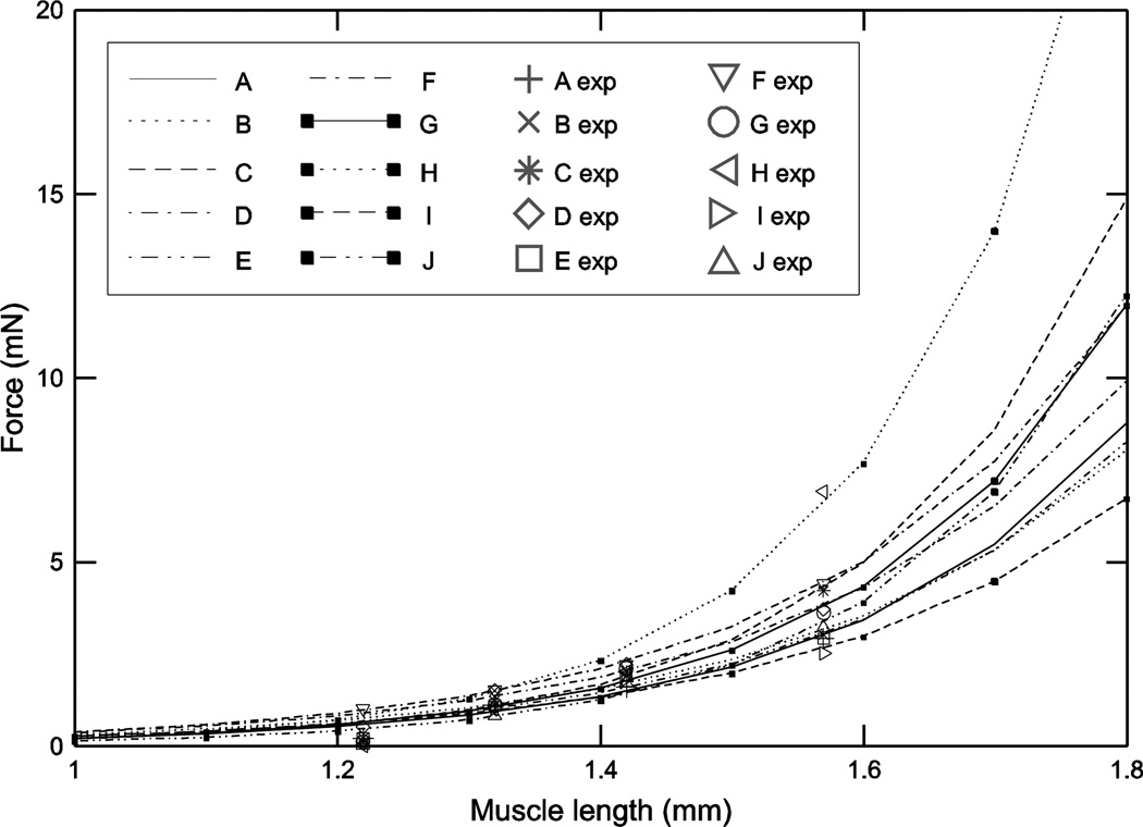
where FP is muscle force, k1 and k2are the fit parameters, and LM is muscle fiber length. Muscle fiber length was set to muscle length because the pinnation angle of the extensor muscle fibers is small enough that ignoring it caused maximum errors in muscle fiber length estimation of less than 4% (see Materials and Methods of Blümel et al. 2011a). Because of the exponential nature of these curves, the FP range across the 10 muscles was relatively small at small fiber lengths (0.4 to 0.85 mN at a fiber length of 1.21 mm, on the shorter side of the working range) and increased as fiber length increased (3 to 7.6 mN at 1.56 mm, on the longer side of the working range) (Fig. 1). k1 showed much greater variation (12.9-fold) than k2(1.5-fold, Table 1), but changes in k2 have a much greater effect on how force changes with muscle length because of k2’s position in the exponent. Note, for instance, that the steepest curve in the plot, animal H, has the highest k2 value but the second lowest k1 value. This very strong effect of changing k2 can also be appreciated by noting that, although animal H’s curve appears very different from those of the other animals, its k2 value (5.99) was only modestly larger than that of the next-largest k2 (5.73).
Fig. 1.
Passive steady-state force-length curves showed large inter-animal variation, particularly at long muscle lengths. Key identifies which data and curves come from which animal, and is used in all figures (2–11) showing data from multiple animals. Lines (left two columns in key) are curve fit lines, symbols (right two columns in key) are data points.
3.3 Initial length responses of activated muscles to rapid force changes
Applying step changes in holding force to muscles producing steady-state isometric force (induced by motor nerve stimulation) resulted in a rapid initial length change followed by a slow change to a final steady state length (see Blümel et al 2011a for a description of how these regions were defined). The initial changes are often modeled as arising from instantaneous length changes of a spring in series with the contractile element (e.g., Jewell and Wilkie 1958) and were well modeled with a quadratic spring equation,
| (2) |
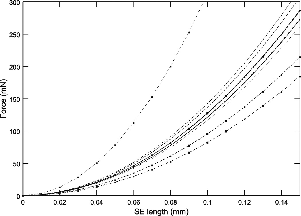
where k3 is the spring constant and LSE is series elastic element length. The FSE curves calculated from these k3 values again resulted in large force variation across the ten muscles examined (Fig. 2), with the differences between the curves again increasing with muscle length, and large variation (8 to 31 N/mm2, 3.8-fold, with all the data; 8 to 14.2 N/mm2, 1.8-fold, if the ‘31’ is deleted as an outlier) in k3 (Table 1).
Fig. 2.
Initial length responses to rapid force changes (‘series elasticity’) showed large inter-animal variation. Note that the top curves in Figs. 1 and 2, which are from the same animal, are neither the largest or smallest curves in Figs. 3–11.
3.4 Rest length force-activation curve
The force the muscles produced at rest length when the motor nerve was stimulated at multiple frequencies (act, normalized to 200 Hz) was modeled with a Gompertz equation,
| (3) |
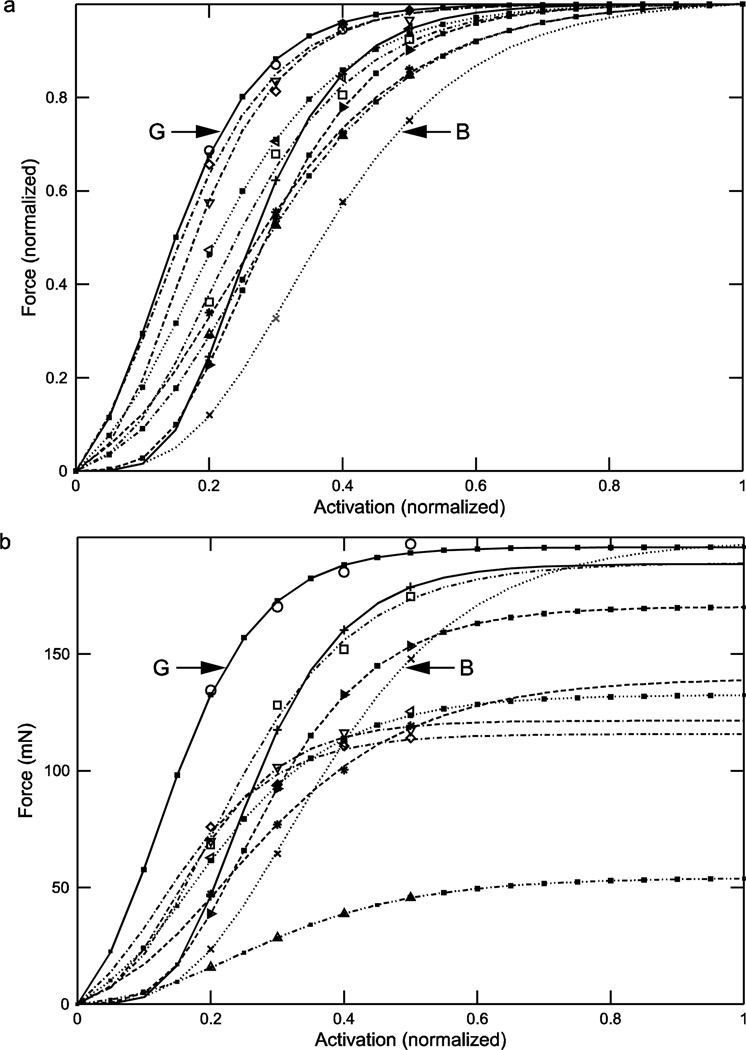
where Fmax, A, and B are parameters determined from the fits. Figure 3a shows the curves normalized to each muscle’s Fmax and Fig. 3b the curves multiplied by each muscle’s Fmax to give actual muscle force. Even when inter-muscle maximum force differences have been removed (Fig. 3a), large differences in curve shape are apparent. For instance, the activation levels at which the various curves reach half-maximal force (0.5) ranged from 0.15 (muscle G) to 0.38 (muscle B), 2.5-fold. These changes were due solely to the different muscles having different A and B parameter values, ranging from 6.3 to 11.4 (A, 1.8-fold) and 0.12 to 0.32 (B, 2.7-fold) (Table 1). Incorporating the various Fmax values of the muscles (Fig. 3b) increased the variation between the curves, with Fmax varying from 54 to 197 mN (3.7-fold, Table 1). Note that there was no correlation between Fmax and the activation level at which half-maximal force occurs, as is well shown by the Fmax values of muscle G and B being nearly identical (196 vs. 197 mN) despite their normalized half-maximal force values being the most different of all the ten muscles.
Fig. 3.
Normalized (panel a) and real (panel b) rest length force-activation showed large inter-animal variation. Incorporating real force increased inter-animal variability. No obvious correlation between muscle maximum force and other curve characteristics (e.g., at what activation the muscles achieve half-maximal force) was apparent. ‘G’ and ‘B’ identify curves arising from two of the muscles (see Table 1 and Results).
3.5 Force-length curves at all activations
Muscle force at all lengths and activations was modeled with the following equations:
| (4) |
| (5) |
| (6) |
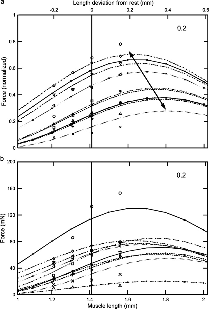
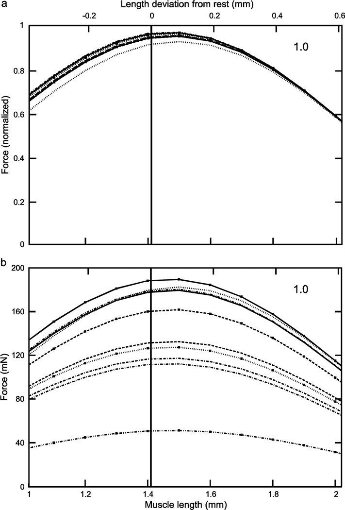
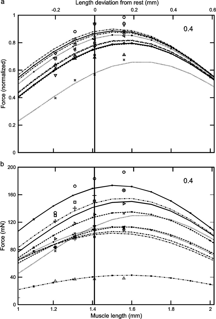
These equations are described in detail in Blümel et al. 2011a. In brief, ω both determines at which LM the sine wave in the square brackets in eqn. 4 has its maximum value, and scales, through eqn. 4’s Aact term and eqns. 5 and 6, normalized muscle force (FL) as a function of muscle activation (act, normalized to 200 Hz). The additional terms in the square brackets in eqn. 4 ensure that the value of the square bracket is positive for all LM and zero on all curves at the same point (Lm = 2.7 mm) on their descending arms. Aact is an exponential function of ω. ω is a hyperbolic function of act, with the parameter curvω determining hyperbola curvature. curvω is the only parameter that is fitted, using normalized muscle force data at various muscle lengths and motor nerve stimulation frequencies. These fits resulted in curvω values such that FL was always a single-peaked positive function in the muscle’s physiological length range of 1.1 to 1.7 mm (‘a’ panels of Figs. 4–6). Real forces (‘b’ panels of Figs. 4–6) were obtained by multiplying eqn. 4 with each muscle’s Fmax.
Fig. 4.
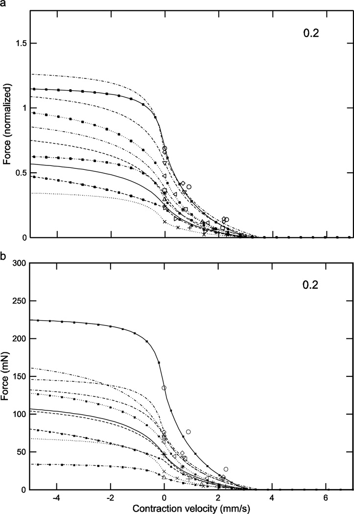
Normalized (a) and real (b) force-length curves showed large inter-animal variation (data for an activation of 0.2 shown here; see Figs. 5 and 6 for the data for activations of 0.4 and 1.0). In the normalized data increasing activation reduced 1) the variation in the lengths at which peak force occurred (double-headed arrow in panel ‘a’; at an activation of 0.2 these lengths varied, depending on the muscle, from 1.61 to 1.84 mm whereas at an activation of 1.0 (Fig. 6a) maximum force occurred at a length of 1.49 mm for all muscles) and 2) the variation in maximum force (compare ‘a’ panels of Figs. 4–6; at an activation of 0.2 normalized maximum force varied, depending on the muscle, from 0.28 to 0.69 whereas at an activation of 1.0 (Fig. 6a) normalized maximum force varied only from 0.93 to 0.98). Multiplying normalized force by each muscle’s Fmax to give real force (panel ‘b’) introduced curve crossings at the 0.2 (this figure) and 0.4 (Fig. 5b) activations and removed the reduction in variability with increased activation seen in the normalized data (‘a’ and ‘b’ panels in Figs. 5 and 6; in both figures across-muscle variation in normalized force was small but across-muscle variation in real force was large). Numbers in right upper corner in each panel are activation level. In both panels top × axes are length deviation from rest and bottom × axes are muscle length.
Fig. 6.
Normalized (a) and real (b) force-length curves showed large inter-animal variation (data for an activation of 0.6 shown here; see Figs. 4 and 5 for the data for activations of 0.2 and 0.4). In the normalized data increasing activation reduced 1) the variation in the lengths at which peak force occurred (double-headed arrow in Fig. 4a; at an activation of 0.2 (Fig. 4a) these lengths varied, depending on the muscle, from 1.61 to 1.84 mm whereas at an activation of 1.0 (Fig. 6a) maximum force occurred at a length of 1.49 mm for all muscles) and 2) the variation in maximum force (compare ‘a’ panels of Figs. 4–6; at an activation of 0.2 (Fig. 4a) normalized maximum force varied, depending on the muscle, from 0.28 to 0.69 whereas at an activation of 1.0 (Fig. 6a) normalized maximum force varied only from 0.93 to 0.98). Multiplying normalized force by each muscle’s Fmax to give real force (panel ‘b’) introduced curve crossings at the 0.2 (Fig. 4b) and 0.4 (Fig. 5b) activations and removed the reduction in variability with increased activation seen in the normalized data data (‘a’ and ‘b’ panels in this figure and in Fig. 5; in both figures across-muscle variation in normalized force was small but across-muscle variation in real force was large). Numbers in right upper corner in each panel are activation level. In both panels top×axes are length deviation from rest and bottom×axes are muscle length.
Considering first the normalized (eqn. 4) curves, at low activation levels the variation in curvω across the ten muscles (3.23, bottom curve, to 6.22, top curve, 1.9-fold range, Table 1) results in large variations in curve shape (e.g., in Fig. 4a, maximum normalized forces range from 0.25 to 0.7 and the lengths at which these maxima occur from 1.6 to 1.8). As activation increases the differences between the curves become smaller, with the normalized curves becoming essentially identical at maximum activation (Fig. 6a). Incorporating the differing Fmax values of the 10 muscles (‘b’ panels of Figs. 4–6) increased across-animal variation (e.g., compare Fig. 6a and 6b) and also caused the curves to cross one another at low to moderate activations (Figs. 4b, 5b), destroying the smooth vertical and leftward displacement with increasing curvω seen in the normalized curves (double-headed arrow, Fig. 4a). Taken together, these data show that at low activation levels inter-muscle differences in both curvω and Fmax contribute to the different real force curves seen across the muscles, but at high activation levels the differences between the muscles are due only to their differing Fmax values.
Fig. 5.
Normalized (a) and real (b) force-length curves showed large inter-animal variation (data for an activation of 0.4 shown here; see Figs. 4 and 6 for the data for activations of 0.2 and 1.0). In the normalized data increasing activation reduced 1) the variation in the lengths at which peak force occurred (double-headed arrow in Fig. 4a; at an activation of 0.2 (Fig. 4a) these lengths varied, depending on the muscle, from 1.61 to 1.84 mm whereas at an activation of 1.0 (Fig. 6a) maximum force occurred at a length of 1.49 mm for all muscles) and 2) the variation in maximum force (compare ‘a’ panels of Figs. 4–6; at an activation of 0.2 (Fig. 4a) normalized maximum force varied, depending on the muscle, from 0.28 to 0.69 whereas at an activation of 1.0 (Fig. 6a) normalized maximum force varied only from 0.93 to 0.98). Multiplying normalized force by each muscle’s Fmax to give real force (panel ‘b’) introduced curve crossings at the 0.2 (Fig. 4b) and 0.4 (this figure) activations and removed the reduction in variability with increased activation seen in the normalized data data (‘a’ and ‘b’ panels in this figure and in Fig. 6; in both figures across-muscle variation in normalized force was small but across-muscle variation in real force was large). Numbers in right upper corner in each panel are activation level. In both panels top × axes are length deviation from rest and bottom × axes are muscle length.
3.6 Force-velocity curve
Force-velocity curves construction is again explained in detail in Blümel et al. 2011a. In brief, force-velocity was modeled using different normalized force equations for shortening (eqn. 7) and lengthening (eqn. 8) contractions,
| (7) |
| (8) |
where both equations are modifications of the classic Hill (1938) hyperbola, the e−e−A·(act–B) terms ensure that the curves meet at zero velocity, cpos is 0.5 (Guschlbauer et al. 2007), and vmax neg and cneg are constants determined from fits to the data. vmax pos, alternatively, is a function of activation that was independently modeled using
| (9) |
where vmax (act=1) is a fit parameter and the ‘0.3’ term comes from Guschlbauer et al. 2007. Real forces were obtained by multiplying eqns. 7 and 8 by each muscle’s Fmax.
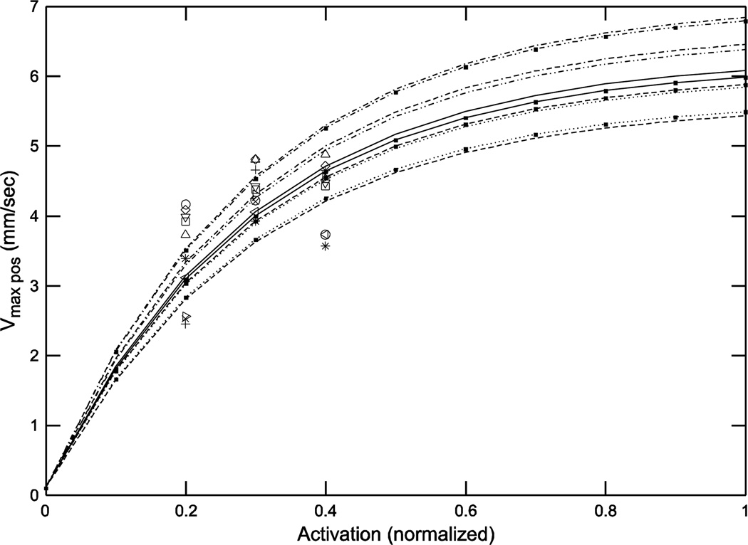
Considering first eqn. 9, since the curvature of the vmax pos curves is fixed (0.3), only their amplitude can vary. The variation is therefore small at low activations and increases with activation (Fig. 7), with a range at maximum activation (1) of 5.4 to 6.8 (1.3-fold), similar to the variation of the vmax (act=1) parameter (5.6 to 7.05, 1.3-fold) (Table 1).
Fig. 7.
At large activations vmax pos showed large inter-animal variation.
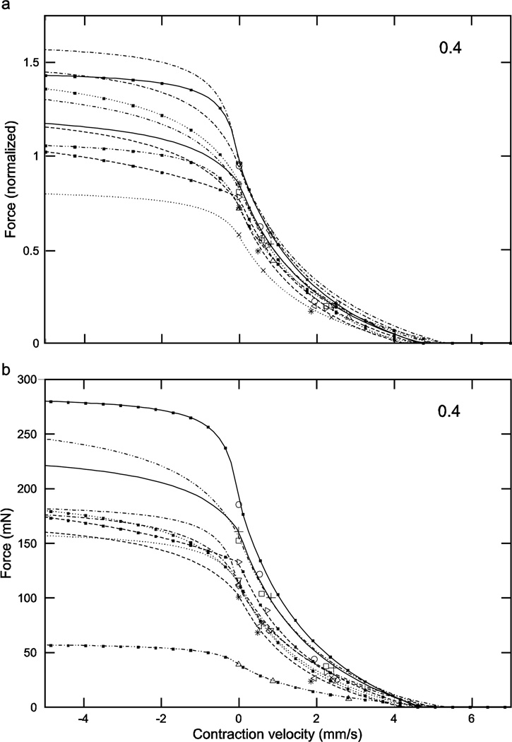
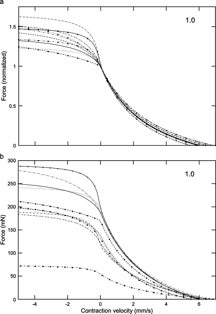
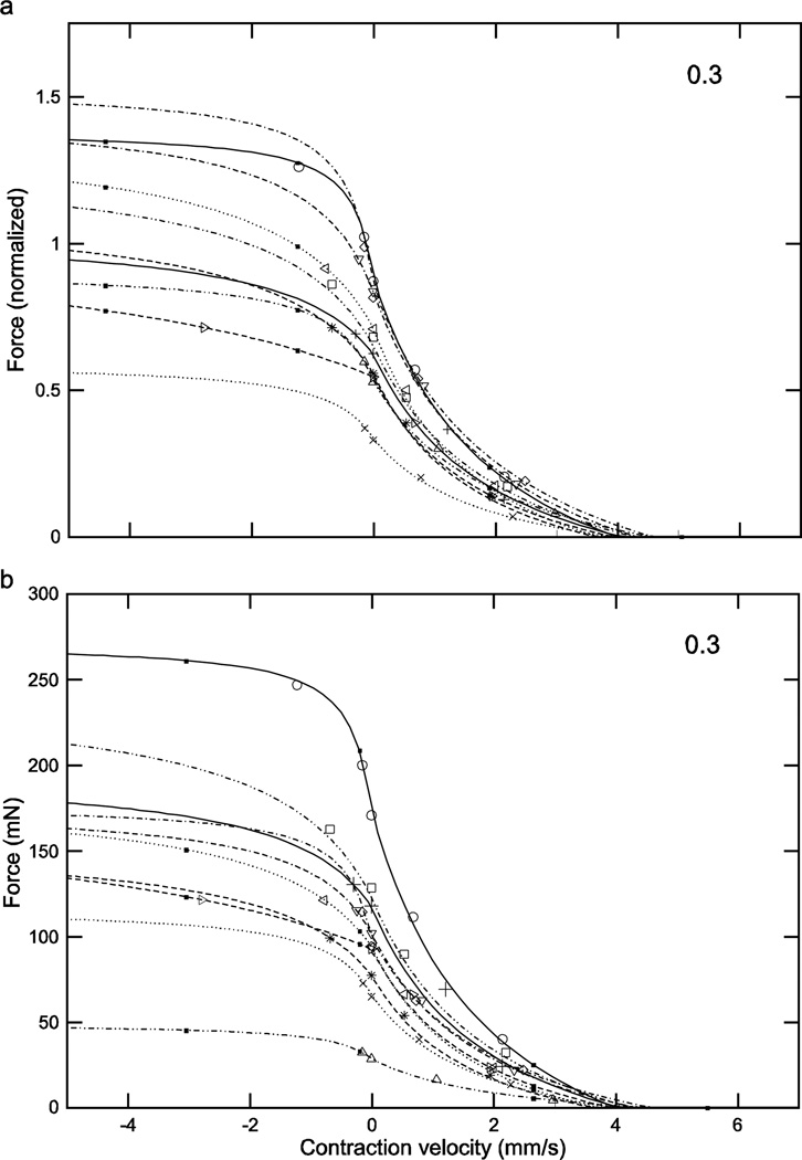
With respect to eqns. 7 and 8 (‘a’ panels of Figs. 8–11), these normalized force curves were similar to those in Figs. 4–6 in that the variation between them decreased as activation increased. At low activation levels the curves showed substantial differences, with the force at 0 velocity ranging from 0.1 to 0.7 (7-fold). Incorporating the muscle’s differing Fmax values (‘b’ panels of Figs. 8–11) removed this increasing similarity with increasing activation, with the curves even at an activation of 1 having a force range at 0 velocity of 54 to 197 mN (3.7-fold). With respect to the fitted parameters in eqn. 8 (the only ones fitted in eqns. 7 and 8), the ranges were 0.23 to 3.99 (17-fold) for vmax neg using all the data or 0.23 to 1.07 (4.6-fold) assuming that the ‘3.99’ was an outlier, and −1.26 to –1.68 for cneg (1.3-fold).
Fig. 8.
Normalized (a) and real (b) force-velocity curves showed large inter-animal variation (data for an activation of 0.2 shown here; see Figs. 9–11 for the data for activations of 0.3, 0.4, and 1.0). Similar to the case for the force-length curves at all activations (Figs. 4–6), in the normalized data inter-animal variability decreased as activation increased, but incorporation of the real forces removed this decrease. Numbers in right upper corner in each panel are activation level. To preserve figure legibility, velocities less than −5 mm/s (9 data points) are not shown.
Fig. 11.
Normalized (a) and real (b) force-velocity curves showed large inter-animal variation (data for an activation of 0.2 shown here; see Figs. 8–10 for the data for activations of 0.2, 0.3, and 0.4). Similar to the case for the force-length curves at all activations (Figs. 4–6), in the normalized data inter-animal variability decreased as activation increased, but incorporation of the real forces removed this decrease. Numbers in right upper corner in each panel are activation level. To preserve figure legibility, velocities less than −5 mm/s (9 data points) are not shown.
3.7 Parameter correlations
A Spearman rank test of the 10 parameters across the 10 muscles identified two significantly-correlated parameter pairs, k1 and k2 of the passive steady-state forcelength curve (section 3.2) and parameter B of the rest length force-activation curve (section 3.4) and curvω of the force-length curve at all activations (section 3.5).
3.7.1 k1 and k2 parameter correlation
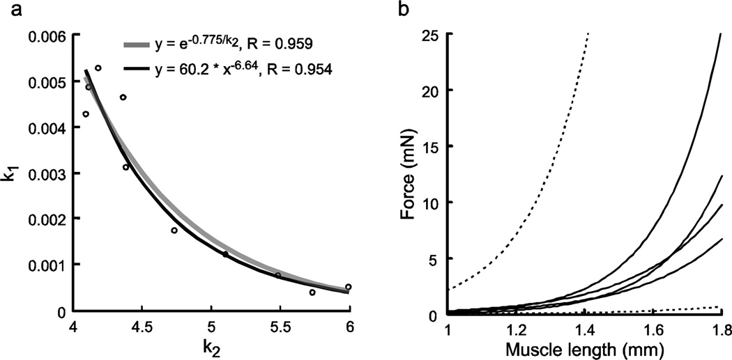
Plotting k1 vs. k2 showed that these two parameters are very well fit with power law or exponential relationship, with k1 decreasing as k2 increases (Fig. 12a). The curves in Fig. 1 and the effects of changing k1 and k2 suggest that this correlation limits intermuscle variation of the passive steady-state force-length curves. The solid lines in Fig. 12b plot the four curves in Fig. 1 that have the largest and smallest k1 values and the largest and smallest k2 values. The upper dashed line is the curve that would result from using the largest k1 value and largest k2 value and the lower dashed line is the curve that would result from using the smallest k1 value and smallest k2 value in eqn. 1. The actual curves occupy a much smaller area than that bordered by the dashed lines. Equation 1 shows that, at any fiber length, decreasing either k1 or k2 will decrease curve amplitude and increasing either k1 or k2 will increase curve amplitude. The amplitude of the passive steady-state force-length curve of a muscle with a large k1 can thus be decreased by decreasing k2, and one with a large k2 by decreasing k1. Similarly, the amplitude of the passive steady-state force-length curve of a muscle with a small k1 can be increased by increasing k2, and one with a small k2 by increasing k1. An inverse relationship between k1 and k2 thus decreases the effects of changes in either parameter on passive steady-state force-length curve amplitude. This negative correlation limits the passive steady-state force-length curves of the various muscles to a relatively small region despite the wide inter-muscle variation in k1 and k2.
Fig. 12.
Across animal-correlation of k1 and k2 parameters of the passive force length curve (a) and possible explanation (b). a, k1 and k2 were well correlated by negative power law or exponential functions. b, Solid lines show data from muscles with largest and smallest k1 and k2 parameters (Table 1). Upper dashed line shows what curve would result using largest k1 and k2 parameters in data set; bottom dashed line shows curve with smallest k1 and k2 parameters in data set. The correlation in panel a, which in the real curves results in the curves with large k1 values having small k2 values and vice versa, results in the real curves occupying a much small region of panel b than they would without the correlation.
3.7.2 B and curvω correlation
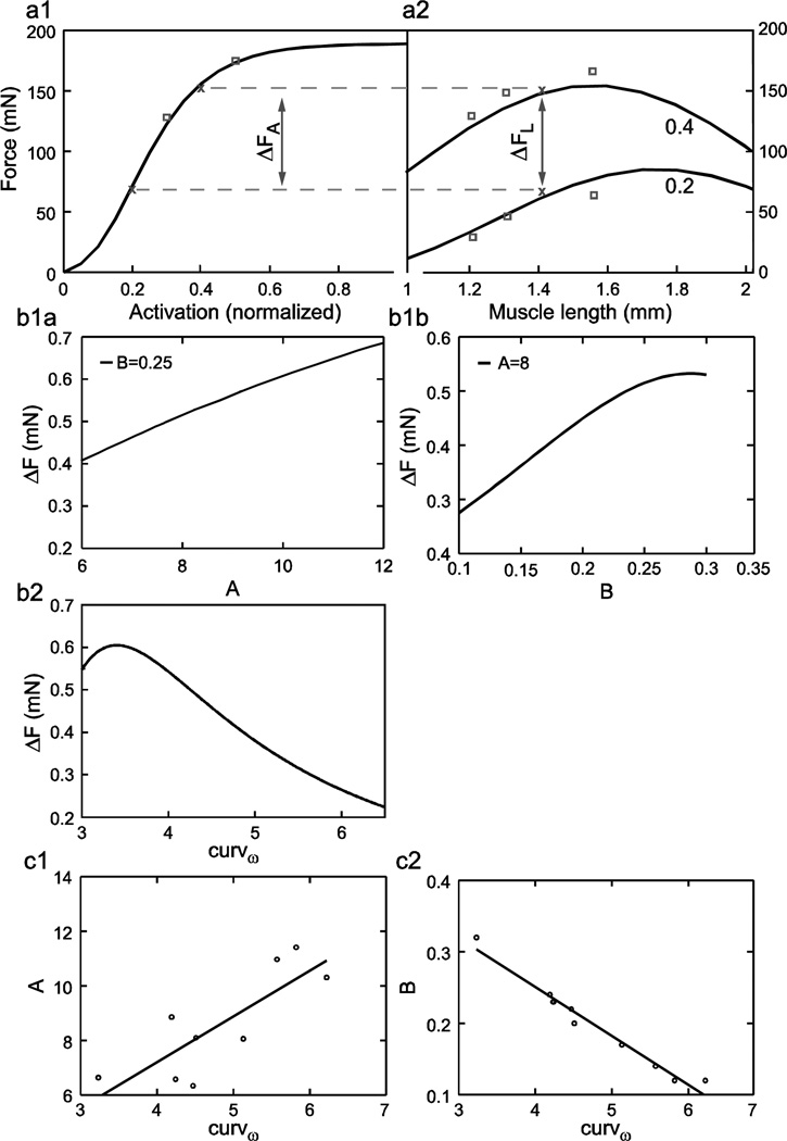
The second correlation, between parameter B of the rest length force-activation curve and curvω of the force-length curves at all activations, likely results from the two curves sharing some common data points in their derivation. Figure 13a1 shows one muscle’s rest length force-activation curve and Fig. 13a2 shows the muscle’s forcelength curves at activations of 0.2 and 0.4. The data points in Fig. 13a2 for rest length are the same as the 0.4 and 0.2 activation data points in Fig. 13a1 at fiber length 1.41 (rest length) (‘x’ data points in both plots). The force difference between the 0.4 and 0.2 activations in Fig. 13a1 (arrow) and the 0.4 and 0.2 activation data points at rest length in Fig. 13a2 (1.41 mm, arrow) must therefore be the same. The data in the two plots are used to fit parameters in different equations (eqn. 3 for the rest length forceactivation curve, eqns. 4–6 for the force-length curves at all activations). The presence of these two identical data points in the two plots does not mean that the corresponding force differences between the fit curves in the two plots will be identical. However, the goodness of the fits (Blümel et al. 2011a) ensures that the fit curves lie very close to all data points. The force differences between the curves will therefore generally be very similar.
Fig. 13.
Possible explanation (a, b) and correlations (c) of parameters A and B and curvω. For explanation of correlation see Results. c1, c2, Parameter A was only weakly (non-significantly with our 0.05 α level), but parameter B was strongly and linearly, correlated with curvω. ‘0.4’ and ‘0.2’ in a2 refer to activation level.
This similarity between the two curves at certain regions of them requires that the fits find parameter values that maintain this similarity, and thus link together the parameters in the two equation sets. The nature of this linkage among A, B, and curvω can be understood by plotting the dependence of these force differences on A and B (eqn. 3) and curvω (eqns. 4–6) (Fig. 13b1a-b2). These plots show that, for almost all of the physiologically relevant ranges (Table 1), as A or B increases the force difference increases, but as curvω increases the force difference decreases. It thus follows that, if curvω increases, the force difference can be kept constant by decreasing parameter A, B, or both, and if curvω decreases, the force difference can be kept constant by increasing parameter A, B, or both. Plotting parameter A (Fig. 13c1) and B (Fig. 13c2) vs. curvω shows that the constant force difference is actually maintained in the rest length force-activation fits (Fig. 13a1) by altering parameter B. Parameter A is weakly correlated with curvω (too weakly to be significant in our correlation search), but this correlation is in the wrong direction to maintain the constant force difference. As such, the decrease in parameter B as curvω increases must be large enough to compensate for both the change in curvω and the associated change (if real) in parameter A.
4 Discussion
We have used our protocol (Blümel et al. 2011a) for determining all the parameters of Hill-type muscle models in experiments on single muscles to measure these parameters in 10 muscles and test for correlations among the parameters. We found substantial inter-individual variation in all model parameters and the curves resulting from them. We also identified two pairs of parameters that were significantly correlated and investigated possible reasons for these correlations.
4.1 Possible experimental or analysis artifacts
A concern in work examining inter-animal variability is that the observed variation does not arise from actual differences across the animals, but instead results from dissection damage or similar experimental artifacts. Several observations argue against this possibility here. First, we used only muscles that showed robust contractions that persisted without substantial decline in force (≤20%) throughout the parameter measurement procedures (Blümel et al. 2011a). Second, it might be expected that the properties of substantially damaged muscle would so change that the Hill-type functions used in the curve fits would no longer well fit the data. However, in all cases (Blümel et al. 2011a) the fits were excellent (R2 values routinely ≥0.95).
Third, the variations produced a graded series of curves, not a division into healthy and damaged muscles that would be expected, at least for substantial damage. Consistent with this interpretation, muscles that are an extreme in one plot, and which might therefore be damaged muscles, are not extremes in the others. This observation is particularly important in comparing Figs. 1 and 8–11, which measure passive and active force, respectively, because one type of damage that might be expected is loss of muscle fibers in the dissection. This would be expected to decrease passive and active muscle force equally. The lack of correlation between these two muscle characteristics thus argues against muscle fiber loss being an explanation for the observed variability. Moreover, the variability continues to be present in normalized force curves, in which loss of muscle fibers would have no effect. Fourth, simpler experiments measuring the response of multiple muscles to identical neural input that lacked the potentially more damaging treatments used here (e.g., quick-release and quick stretch experiments) also show large, graded inter-animal variation (Hooper et al. 2006). Taken together, these arguments suggest that at least much of the observed inter-animal variation is likely because of true inter-animal differences.
With respect to the observed correlations, the extremely good correlations shown in Figs. 12a and 13c2 verify the identifications of the original search among all parameters. A different concern is that the chosen 0.05 α level was too stringent and resulted in weak but still real correlations being missed. Fig. 13c1 shows one such weak correlation, and the original all-parameter search identified three other weak correlations, one between A and B (R = 0.68), a second between B and cneg (R = 0.75), and a third between curvω and cneg (R = 0.73) (data not shown). It is impossible from our present data to state if these correlations are real or spurious, particularly for the cneg correlations, inasmuch as cneg was determined from only two data points, fewer than the other parameters, and measuring this parameter is more difficult experimentally than are the others (see Materials and Methods, Blümel et al. 2011a).
4.2 Implications of the observed correlations
k1 and k2 are negatively correlated with a power law or exponential relationship. This correlation has the effect of limiting passive force-length curve variation. This observation raises the question of whether power-law or exponential parameter covariation is particularly well-suited to limiting exponential function amplitude variation. Regardless, an important point to make about this correlation, and indeed all the functions in the phenomenological modeling used here, is that one cannot infer biological mechanism from them. That is, the negative power-law or exponential correlation of k1 and k2 does not imply the existence of two biological processes (e.g., concentrations of two proteins), one represented by k1 and the other k2, whose expression is inversely and power-law or exponentially linked.
The correlation between curvω and B likely arises solely from a model-inherent connection. In retrospect, since the force-activation at rest length curve (Fig. 3) is a subset of the force-length at all activation curves (Figs. 4–6), it is obvious that having both these functions in the model was redundant. Indeed, in model simulations (Blümel et al. 2011b), we do not use the force-activation at rest length curve as its purpose is completely fulfilled by the force-length at all activation curves. However, it is an important part of model building because its data very accurately specify Fmax, a central model parameter not well specified by the force-length at all activation curves.
4.3 Implications of inter-animal variability for neural control
Muscles drive movement. The wide variability shown here suggests that, to produce identical movements in different animals, neural input would need to be specifically matched to muscle properties. Although this is undoubtedly theoretically true, it is possible that, in practice, movements, at least in the stick insect, are not controlled on this level of detail. Although this concept may run counter to implicit assumptions in much motor control work, such ‘just-good-enough’ movement control has been observed in other systems, notably Aplysia feeding movements, which are not matched to type of food being eaten and show great bite-to-bite variability even when eating a single food type (Horn et al. 2004, summarized in Hooper 2004). Another possibility is that compensatory changes in antagonist muscle passive resistance or joint or limb properties (Hooper et al. 2009) reduce the effects of inter-animal extensor muscle variation sufficiently that these variations do not result in functionally different movements in response to identical neural input, and thus matching of neural input and muscle characteristics is again unnecessary.
4.4 Implications of inter-animal variability for modeling
Muscles and neurons are typically modeled using means obtained from averaging across many animals. Such averaging approaches are only assured of success if there is relatively little across-animal variation in these fundamental system characteristics (Golowasch et al. 2002; Blümel et al. 2011a). The large variations in the values of these characteristics reported here suggest that quantitatively accurate stick insect muscle models may need to be constructed on an individual-by-individual basis. The final test of this possibility is comparison of individual muscle-specific models vs. models constructed with averaged parameter values. We show in the final paper of this series that muscle-specific modeling decreases model error some 50% (Blümel et al. 2011b). There is, a priori, no reason to assume that stick insect extensor muscle is particularly variable across individuals. Similarly large variations in fundamental characteristics may thus be present in other muscles (e.g., as noted earlier, lobster pyloric muscles also show large across-individual variation in whole muscle responses, Thuma et al. 2003). The methods in Blümel et al. 2011a for obtaining individual-specific characterizations, and the tests performed here for correlation between these parameters that such data allow, may thus be relevant for muscle work in a large variety of species.
Fig. 9.
Normalized (a) and real (b) force-velocity curves showed large inter-animal variation (data for an activation of 0.3 shown here; see Figs. 8, 10, and 11 for the data for activations of 0.2, 0.4, and 1.0). Similar to the case for the force-length curves at all activations (Figs. 4–6), in the normalized data inter-animal variability decreased as activation increased, but incorporation of the real forces removed this decrease. Numbers in right upper corner in each panel are activation level. To preserve figure legibility, velocities less than −5 mm/s (9 data points) are not shown.
Fig. 10.
Normalized (a) and real (b) force-velocity curves showed large inter-animal variation (data for an activation of 0.4 shown here; see Figs. 8, 9, and 11 for the data for activations of 0.2, 0.3, and 1.0). Similar to the case for the force-length curves at all activations (Figs. 4–6), in the normalized data inter-animal variability decreased as activation increased, but incorporation of the real forces removed this decrease. Numbers in right upper corner in each panel are activation level. To preserve figure legibility, velocities less than −5 mm/s (9 data points) are not shown.
Acknowledgments
Research supported by a Mercator Guest Professor award to SLH and grants DA1182/1-1 to SG and Bu857/9 to AB, all from the Deutsche Forschungsgemeinschaft.
Symbols and definitions
- A,B,
parameters in rest length force-activation curve (eqns. 3, 7, 8) (unitless)
- Aact
maximum amplitude of force-length curves (eqns. 4, 5) (unitless)
- act
muscle activation (eqns. 3, 6, 7–9) (normalized to 200 Hz, therefore unitless)
- cneg, cpos
curvatures of Hill hyperbola for shortening (eqn. 7) and lengthening (eqn. 8) contractions, respectively (unitless)
- curvω
curvature of hyperbola relating ω and act (eqn. 6) (mm0.5)
- FA
active force at rest length (eqn. 3) (mN)
- FL
active force at different muscle lengths (force-length curve) (eqn. 4) (normalized to Fmax, and therefore unitless)
- Fmax
maximum isometric force at rest length (eqn. 3) (mN)
- FP
steady-state passive force (parallel spring) (eqn. 1) (mN)
- FSE
series elastic spring force (eqn. 2) (mN)
- FV
FL at different contraction velocities (force-velocity curve) (eqns. 7, 8) (normalized to Fmax, and therefore unitless)
- k1, k2
passive steady-state force length curve constants (eqn. 1) (k1, mN; k2, mm−1)
- k3
proportionality constant in quadratic force equation (eqn. 2) (mN/mm2)
- LM
- LSE
series elastic element length (eqn. 2) (mm)
- v
- vmax neg, vmax pos
maximum velocity of muscle length change for shortening (eqns. 7, 9) and lengthening (eqn. 8) contractions, respectively (mm/s)
- vmax(act=1)
vmax pos at an activation of 1 (eqn. 9) (mm/s)
- ω
Contributor Information
Marcus Blümel, Email: bluemelm@uni-koeln.de.
Christoph Guschlbauer, Email: c.guschlbauer@uni-koeln.de.
Silvia Daun-Gruhn, Email: sgruhn@uni-koeln.de.
Ansgar Büschges, Email: Ansgar.Bueschges@uni-koeln.de.
Reference List
- Blümel M, Guschlbauer C, Hooper SL, Büschges A. Determining all parameters necessary to build Hill-type muscle models from experiments on single muscles. 2011a doi: 10.1007/s00422-012-0531-5. [COMPANION ARTICLE] [DOI] [PMC free article] [PubMed] [Google Scholar]
- Blümel M, Guschlbauer C, Hooper SL, Büschges A. Using individual-muscle specific data halves muscle simulation error. 2011b doi: 10.1007/s00422-011-0460-8. [COMPANION ARTICLE] [DOI] [PubMed] [Google Scholar]
- Brown IE, Cheng EJ, Loeb GE. Measured and modeled properties of mammalian skeletal muscle. II. The effects of stimulus frequency on force-length and force-velocity relationships. J Muscle Res Cell Motil. 1999;20:627–643. doi: 10.1023/a:1005585030764. [DOI] [PubMed] [Google Scholar]
- Golowasch J, Goldman MS, Abbott LF, Marder E. Failure of averaging in the construction of a conductance-based neuron model. J Neurophysiol. 2002;87:1129–1131. doi: 10.1152/jn.00412.2001. [DOI] [PubMed] [Google Scholar]
- Guschlbauer C, Scharstein H, Büschges A. The extensor tibiae muscle of the stick insect: biomechanical properties of an insect walking leg muscle. J Exp Biol. 2007;210:1092–1108. doi: 10.1242/jeb.02729. [DOI] [PubMed] [Google Scholar]
- Hannaford B, Winters J. Actuator properties and movement control: biological and technological models. In: Winters JM, Woo SLY, editors. Multiple muscle systems: biomechanics and movement organization. New York, NY: Springer-Verlag; 1990. pp. 101–120. [Google Scholar]
- Hill AV. The heat of shortening and the dynamic constants of muscle. Proc R Soc Lond B Biol Sci. 1938;126:136–195. doi: 10.1098/rspb.1949.0019. [DOI] [PubMed] [Google Scholar]
- Hill AV. The series elastic component of muscle. Proc R Soc Lond B Biol Sci. 1950;141:104–117. doi: 10.1098/rspb.1950.0035. [DOI] [PubMed] [Google Scholar]
- Hooper SL. Variation is the spice of life. J Neurophysiol. 2004;92:40–41. doi: 10.1152/jn.00182.2004. (Focus Horn et al. 2004) [DOI] [PubMed] [Google Scholar]
- Hooper SL, Guschlbauer C, Blümel M, Rosenbaum P, Gruhn M, Akay T, Büschges A. Neural control of unloaded leg posture and of leg swing in stick insect, cockroach, and mouse differs from that in larger animals. J Neurosci. 2009;29:4109–4119. doi: 10.1523/JNEUROSCI.5510-08.2009. [DOI] [PMC free article] [PubMed] [Google Scholar]
- Hooper SL, Guschlbauer C, von Uckermann G, Büschges A. Natural neural output that produces highly variable locomotory movements. J Neurophysiol. 2006;96:2072–2088. doi: 10.1152/jn.00366.2006. [DOI] [PubMed] [Google Scholar]
- Horn CC, Zhurov Y, Orekhova IV, Proekt A, Kupfermann I, Weiss KR, Brezina V. Cycle-to-cycle variability of neuromuscular activity in Aplysia feeding behavior. J Neurophysiol. 2004;92:157–180. doi: 10.1152/jn.01190.2003. [DOI] [PubMed] [Google Scholar]
- Jewell BR, Wilkie DR. An analysis of the mechanical components in frog's striated muscle. J Physiol. 1958;143:515–540. doi: 10.1113/jphysiol.1958.sp006075. [DOI] [PMC free article] [PubMed] [Google Scholar]
- Rack PMH, Westbury DR. The effects of length and stimulus rate on tension in the isometric cat soleus muscle. J Physiol. 1969;204:443–460. doi: 10.1113/jphysiol.1969.sp008923. [DOI] [PMC free article] [PubMed] [Google Scholar]
- Ramsey PH. Critical values for Spearman's rank order correlation. JEBS. 1989;14:245–253. [Google Scholar]
- Schulz DJ, Goaillard J-M, Marder E. Variable channel expression in identified single and electrically coupled neurons in different animals. Nat Neurosci. 2006;9:356–362. doi: 10.1038/nn1639. [DOI] [PubMed] [Google Scholar]
- Thuma JB, Morris LG, Weaver AL, Hooper SL. Lobster (Panulirus interruptus) pyloric muscles express the motor patterns of three neural networks, only one of which innervates the muscles. J Neurosci. 2003;23:8911–8920. doi: 10.1523/JNEUROSCI.23-26-08911.2003. [DOI] [PMC free article] [PubMed] [Google Scholar]
- Wilkie DR. Measurement of the series elastic component at various times during a single muscle twitch. J Physiol. 1956;134:527–530. doi: 10.1113/jphysiol.1956.sp005662. [DOI] [PMC free article] [PubMed] [Google Scholar]
- Winters JM. Hill-based muscle models: a systems engineering perspective. In: Winters JM, Woo SLY, editors. Multiple muscle systems: biomechanics and movement organization. New York: Springer-Verlag; 1990. pp. 69–93. [Google Scholar]
- Zahalak GI. Modeling muscle mechanics (and energetics) In: Winters JM, Woo SLY, editors. Multiple muscle systems: biomechanics and movement organization. New York, NY: Springer-Verlag; 1990. pp. 1–23. [Google Scholar]
- Zajac FE, Winters JM. Modeling musculoskeletal movement systems: joint and body segmental dynamics, musculoskeletal actuation, and neuromuscular control. In: Winters JM, Woo SLY, editors. Multiple muscle systems: biomechanics and movement organization. New York: Springer-Verlag; 1990. pp. 121–148. [Google Scholar]


