Abstract
Previous studies have shown that by minimizing the total variation (TV) of the to-be-estimated image with some data and other constraints, a piecewise-smooth X-ray computed tomography (CT) can be reconstructed from sparse-view projection data without introducing noticeable artifacts. However, due to the piecewise constant assumption for the image, a conventional TV minimization algorithm often suffers from over-smoothness on the edges of the resulting image. To mitigate this drawback, we present an adaptive-weighted TV (AwTV) minimization algorithm in this paper. The presented AwTV model is derived by considering the anisotropic edge property among neighboring image voxels, where the associated weights are expressed as an exponential function and can be adaptively adjusted by the local image-intensity gradient for the purpose of preserving the edge details. Inspired by the previously-reported TV-POCS (projection onto convex sets) implementation, a similar AwTV-POCS implementation was developed to minimize the AwTV subject to data and other constraints for the purpose of sparse-view low-dose CT image reconstruction. To evaluate the presented AwTV-POCS algorithm, both qualitative and quantitative studies were performed by computer simulations and phantom experiments. The results show that the presented AwTV-POCS algorithm can yield images with several noticeable gains, in terms of noise-resolution tradeoff plots and full width at half maximum values, as compared to the corresponding conventional TV-POCS algorithm.
Keywords: Low-dose computed tomography, total variation, adaptive-weighted total variation, sparse-sampled data, image reconstruction
I. Introduction
In view of the negative effects of X-ray exposure to patients, minimizing the exposure risk has been one of the major endeavors in current computed tomography (CT) examinations [1, 2]. Up to now, many hardware-based optimal data-acquisition protocols has been proposed for dose reduction [3, 4, 5]. In the meanwhile, many software-based optimal technologies have been introduced to process low-dose data acquired from available CT scanners without hardware modification. It is well-known that lowering the X-ray exposure (by lower X-ray tube current–measured by milliampere-seconds (mAs), lower X-ray tube voltage–measured by kilovoltage-peak (kVp), or less projection views–measured by the number of views per rotation, i.e., data sparsity) will unavoidably increase the data noise and/or the data inconsistence associated with the sparsity. As a result, high-quality diagnostic CT images cannot be yielded if no adequate handling of the data noise and/or the data inconsistence is applied during image reconstruction. Various image processing and reconstruction methods with noise suppression capability for the purpose of dose reduction have been reported [6, 7, 8].
As one of the major strategies for low-dose CT image reconstruction, restoring the line integrals from acquired low-mAs projection data have been explored [7, 8, 9]. For example, Lu et al. investigated the noise property of low-mAs CT sinogram data by analyzing repeatedly-scanned data from a commercial CT scanner, and correspondingly presented a transform-based method to restore the line integrals from the low-mAs scans [7]. Later, a nonlinear relationship between the variance and the mean of the acquired low-mAs sinogram data was determined by Li et al. [8], which provides a reasonable theoretical prediction of the variance of the projection data to facilitate the low-dose CT image reconstruction. Based on the relationship, Wang et al. [9] investigated a framework of image reconstruction from the low-mAs sinogram data by minimizing the penalized re-weighted least-squares (PRWLS). The restoration principle can be applicable to acquired low-kVp scans. While they were not intended for low-dose CT applications, La Rivière et al. presented an interesting penalized likelihood sinogram restoration algorithm [10] and Elbakri and Fessler reported a series of sophisticated CT image reconstruction algorithms in general [11, 12].
Another major strategy, which could be applied for CT dose reduction, is to reduce the number of projection views per rotation around the body. In current CT exanimations, several hundred or even over a thousand of projections per rotation are acquired. Reducing the number by a half would cut the radiation by a half. In 2006, Donoho proposed the concept of Compressed Sensing (CS) [13], which proves that an image of sparse signals could be satisfactorily reconstructed from far less measurements than what is usually considered necessary, according to the Nyquist sampling theorem, when the associated transfer matrix of the sparse signals satisfy some conditions (such conditions were later described as the restricted isometry property (RIP) [14]). In the same year of 2006, Candès et al. introduced the CS concept into the K-space for image reconstruction in magnetic resonance imaging by solving the l1-norm optimization problem [15]. Furthermore, if a previous image with high similarity to the to-be-estimated image can be introduced into the cost function, the data samples for satisfactory image reconstruction can be further reduced [16, 17, 18, 19]. However, for CT image reconstruction, particularly in low-dose CT applications, the associated transfer matrix of sparse signals in the transfer domain is less likely to have the RIP [20, 21]. Furthermore, except for parallel beam geometry, the central slice theorem, which describes the direct connection between the projection data and the transformed data in the frequency domain in tomographical imaging, may not exist for non parallel geometries such as fan and cone beam geometries and, therefore, an exact implementation of the CS theorem for low-dose CT may not be feasible. Alternative means to reduce the number of projections seems to be needed.
In 1992, Rudin et al. reported that the total variation (TV) norm of the to-be-estimated solution is essentially the l1-norm of derivatives, and they further showed that this norm can be utilized to address the ill-posed image restoration problem [22]. In 2006, Sidky et al. adapted the concept of TV minimization to consider the piecewise constant or sparse source distribution and formulated an innovative algorithm, called TV-POCS (projection onto convex sets), to perform CT image reconstruction from sparse-sampled or sparse-view projection data [20]. Later in 2008, Sidky et al. presented an updating algorithm, i.e., the adaptive-steepest-descent-POCS (ASD-POCS) [21], for TV minimization with improved robustness against the cone-beam artifacts from sparse or limited projection-views with comparison to other classical methods, e.g., the well-known EM algorithm. This ASD-POCS algorithm, simply called TV-POCS hereafter, can be considered as a new attempt to reconstruct images of sparse signals from under-sampled projection data for CT applications. Although the images reconstructed by the TV-POCS algorithm from sparse-sampled data are close to the true source distributions, over-smoothing in the reconstructed image is frequently seen due to the assumption of isotropic edge property in calculating the TV term. Recently, a TV-based edge preserving (EPTV) model [23] was proposed to address the issue of the original TV, and was claimed to preserve edges by bringing in different weights in the TV term from edges and constant areas of the to-be-estimated image.
In this paper, different with the EPTV model, we consider the anisotropic (rather than isotropic) edge property of an image and propose a novel adaptive-weighted TV (AwTV) model for low-dose CT image reconstruction from sparse-sampled projection data. In order to achieve a reasonable balance between resolution and contrast-to-noise ratio in the reconstruction, the associated weights in the AwTV model are expressed as an exponential function, which can be adaptively adjusted with the local image-intensity gradient for the purpose of preserving the edge details. Inspired by the TV-POCS implementation [20, 21], a similar implementation, called AwTV-POCS, is developed to minimize the AwTV with subjection to data and other constraints for the purpose of dose reduction via CT image reconstruction from sparse data.
The remainder of this paper is organized as follows. In Section II, the AwTV model and its associated cost function are presented, and then the POCS-based image reconstruction algorithm for solving the constrained AwTV minimization problem is described. In Section III, experimental results are reported. Finally, discussions and conclusions are given in Section IV.
II. Method
In this section, two CT imaging models with the conventional TV and the presented AwTV minimizations are introduced respectively, and then the corresponding optimization strategy with POCS, i.e., the TV-POCS and AwTV-POCS algorithms, are described in detail.
2.1. CT Imaging Model with the Conventional TV Minimization
For CT image reconstruction from sparse-view or sparse-sampled data, the classic filtered back-projection (FBP) method always suffers from noticeable artifacts due to ill condition of the measured data [20, 21]. To mitigate the ill condition, a satisfactory CT image may be yielded from sparse-viewed data by solving the following constrained optimization problem [20, 21]:
| (1) |
where the TV of the to-be-reconstructed image, i.e., ‖μ‖TV, is defined as:
| (2) |
where μ denotes the vector of attenuation coefficients of the object with μ ∈ M, wherein the object is discretized on a two-dimensional (2D) grad of M image elements or voxels, s and t are the indices of the location of the attenuation coefficients, p represents the linearized or log-transformed projections data, A is the system matrix which depends on the projection geometry [24], and its elements are usually modeled as the intersecting lengths of a ray path with the associated voxels on the path. Because many factors may cause inconsistency between the measurements and the desired data conditions, such as missing data and presence of noise in the measurements, the inequality constraint in (1) is used to control the data fidelity with an error tolerance factor ε. In practice, with the expectation of the l1-norm measure between the acquired and the desired projection data under the tolerance of ε, an optimal solution within the feasible region of minimizing the TV term may be found by the use of an optimization strategy [20, 21].
2.2. CT Imaging Model with the Presented AwTV Minimization
In theory, the conventional TV term in the cost function (1) is based on the assumption of piecewise constant distribution for the desired image, and the assumption often leads to the associated cost function optimization suffering from over-smoothing on the edges in the reconstructed images. Meanwhile, the edge details are vital information for diagnosis in clinic. In order to mitigate the over-smoothing of edges in the conventional TV minimization, a new imaging model with AwTV minimization is proposed as follows:
| (3) |
where the AwTV of the to-be-reconstructed image, i.e., ‖μ‖AwTV, is defined as:
| (4) |
| (5) |
where δ in the weights (Ws,s−1,t,t and Ws,s,t,t−1) is a scale factor which controls the strength of the diffusion during each iteration [25,26].
By the form of AwTV in (4), it is possible to fully consider the gradient of the desired image and also to include the change of local voxel intensities. Specifically, for a smaller change of voxel intensity, a stronger weight can be given; whereas for a larger change of voxel intensity, a weaker weight may be given. Through this diffusion-type weighting process, an adaptive smoothing is encouraged in reference to the difference between neighboring voxels’ intensities. From the viewpoint of scale-space in the diffusion framework, the AwTV of the desired image will no longer be linearly and uniformly calculated for each diffusion direction from a voxel, rather the calculation will be adaptive to the local information of the image with an exponential form. Intuitively, the AwTV model of (4) approaches to the conventional TV model of (2) as the weight goes to 1, thus the TV model may be considered as a special case of the AwTV model when δ → ∞.
2.3. Brief Review of the POCS Strategy and the TV-POCS Algorithm
The POCS strategy is a general iterative scheme to solve linear equations by successive and repeated applications of several projection operators. This strategy was investigated by Sidkey et al. [20, 21] as a possible way to solve the constrained minimization problem of (1), named TV-POCS algorithm. Two independent operating steps are involved in the implementation of their algorithm. In the first step, an initially estimated image is updated iteratively by the POCS strategy. This step is basically the operation of the well-known Algebraic Reconstruction Technique (ART). For illustration purpose, we adopt the Simultaneous ART (SART) [27, 28] to solve the under-determined linear system of (1). More specifically, the SART algorithm is used to yield an image estimate from the initially estimated image by minimizing the distance between the measured and estimated projection data. The associative update scheme can be described as follows:
| (6) |
| (7) |
| (8) |
| (9) |
where Ai, j is an M×N system matrix according to the projection geometry [24] (M was defined before as the total number of image voxels and N is the total number of data samples). ω is a relax parameter for updating the current estimate of the image. k indicates the iterative number. Through the SART algorithm, the initially estimated image is updated iteratively to fulfill the data constraints and an intermediate image is yielded for further update by the second step below.
The second step of the TV-POCS algorithm updates iteratively the intermediate image estimated from the above first step to minimize the TV of the to-be-estimated image. Although many numerical methods can be implemented in this second step to solve the TV minimization problem, such as the TV superiorization strategy [29] and the surrogate TV term strategy [30], we adapt the same gradient decent strategy as described in the TV-POCS algorithm [20, 21] to avoid any bias on the results that may be caused by using different numerical calculating methods for the purpose of comparing the conventional TV and the presented AwTV models. In order to achieve a reasonable optimization solution, some stop criterions should be considered in the iterative process (to be discussed later).
2.4. Presentation of the AwTV-POCS Algorithm
Due to the nonlinear form of the AwTV with respect to the image intensity, it is numerically difficult to utilize directly the second-order derivative for the purpose of effectively minimizing the objective function (3). Inspired by the optimization strategy as described in [31], the weights can be pre-computed at current iteration for the AwTV minimization at the next iteration. By this strategy, the gradient descent technique is adapted to minimize the AwTV of the SART-estimated intermediate image where only the first-order derivative of the AwTV term respect to each voxel value is needed, which can be approximately expressed as:
| (10) |
where ξ is a relax parameter introduced to avoid the denominator going to zero.
Similar to the ASD-POCS approach [21], the optimization of the objective function (3) is implemented by the following iterative scheme, named as AwTV-POCS algorithm. For an image with the array size of S×T, each of the general iterations of I cycles includes J iteration cycles of POCS operation and K iteration cycles of AwTV minimization by gradient descent. The relax parameter ω in the POCS operation decreases as the iteration increases and the step-size τ of the gradient descend also decreases as the iteration increases. Summarily, the pseudo-code for the presented AwTV-POCS algorithm is listed as follows:
| 1: | initial : ; s = 1, 2,…, S, t = 1, 2,…, T; |
| 2: | initial : δ, ε, τ; ω = 1; |
| 3: | while (stop criterion is not met) |
| 4: | for j = 1, 2,…, J; (POCS) |
| 5: | if j = = 1; |
| 6: | ; |
| 7: | ; s = 1, 2,…, S, t = 1, 2,…, T; |
| 8: | end if |
| 9: | end for |
| 10: | ; s = 1, 2,…, S, t = 1, 2,…, T; |
| 11: | ; s = 1, 2,…, S, t = 1, 2,…, T; |
| 12: | end if |
| 13: | ; s = 1, 2,…, S, t = 1, 2,…, T; |
| 14: | ; s = 1, 2,…, S, t = 1, 2,…, T; |
| 15: | ; |
| 16: | for k = 1, 2,…, K; (AwTV gradient descent) |
| 17: | ; |
| 18: | end for |
| 19: | if dp < ε; |
| 20: | ω ≔ 0.995 × ω; |
| 21: | end if |
| 22: | ; |
| 23 : | calculate the criterion; |
| 24: | τ = τ * 0.995; |
| 25: | end if stop criterion is satisfy |
In line 1, an initial estimate of the to-be-reconstructed image is set to be uniform with voxel value of 1. In line 2, four parameters, δ, ε, ω and τ, are initialized before the iteration starts. Specifically, the error tolerance ε is initialized based on the noise level of the data. The initial value of δ in the weights of AwTV term will be discussed later in the Result Section, and so are the parameters ω and τ. Each outer loop (lines 3–23) is performed by two separated iteration steps, i.e., the POCS (or the SART) (lines 4–12) and the gradient descent for the AwTV minimization (lines 16–18). The weights are pre-computed using latest image estimation in line 15. By setting the weight to 1, the above pseudo-code for the presented AwTV-POCS algorithm is applicable to the TV-POCS algorithm [20, 21]. A brief discussion on the stop criterion for both TV-POCS and AwTV-POCS implementations is given below.
2.5. Stop Criterion for Implementation of the AwTV-POCS and TV-POCS Algorithms
In order to ensure the solution of the objective function (3) obtained by the above presented AwTV-POCS implementation is an optimal estimate, the associative Karush-Kuhn-Tucker (KKT) condition should be satisfied, similar to that in the TV-POCS implementation, as reported in [21]. For the TV-POCS algorithm implementation, the KKT condition can be satisfied with an indicator factor cα = −1.0 where cα is defined as:
| (11) |
where d⃗TV is a vector of derivative of the TV term, and d⃗data is a vector of derivative of the data constraints using the Lagrangian multiplier. For the presented AwTV-POCS algorithm implementation, a similar indicator factor can also be used to describe the KKT condition for an optimal estimate. As stated in [21], cα = −1.0 is a necessary condition for an optimal solution for the TV minimization with sufficient data constraints. The necessary condition of cα = −1.0 may not be reached unless a great number of iteration cycles are executed, which may not be practical. In the AwTV-POCS algorithm, we discovered that very small or imperceptible changes was noticeable in the reconstructed images when cα went below −0.6. Thus, in our algorithm implementation, we used cα < −0.6 as stop criterion in line 23 of the above pseudo-code.
To evaluate the differences between the resulting images from the AwTV-POCS and TV-POCS approaches, several computer simulation and phantom experiment studies were performed and reported in the following section.
III. Results
For computer simulation studies, a modified Shepp-Logan mathematical phantom was designed based on the mass attenuation coefficients of different tissues in the objects in the phantom. For phantom experiment studies, two sets of cone-beam projection data were acquired from two different types of phantom models, respectively, using a commercial CT scanner. One phantom model is the CatPhan® 600 phantom and the other is an anthropomorphic head phantom. The TV-POCS algorithm [20, 21] was implemented as the baseline or reference for comparison purpose. In addition, the EPTV model with incorporation of the POCS strategy, or EPTV-POCS algorithm, was implemented by using the similar scheme as the TV-POCS algorithm.
3.1. Computer Simulation Studies
For simplicity, without loss of generality, a parallel-beam CT imaging geometry was used for the purpose of measuring the gain of the AwTV minimization with comparison to the conventional TV minimization. This geometry was modeled with 1024 bins on a 1D detector for 2D image reconstruction. The distance between the centers of two neighboring detector elements or bins is 0.25mm. Given the digital phantom, the noise-free transmission data was computed by the use of the Lambert-Beer’s law, ), where p̅i is the line integral of the phantom intensity distribution along the ray i, is the mean number of incident photons. Given the noise-free data, the noisy transmission data were simulated based on the assumption for the statistical model of the measurements (to be discussed later in Section 3.1.2).
3.1.1. Design of a Modified Shepp-Logan Phantom and Computation of Line Integrals
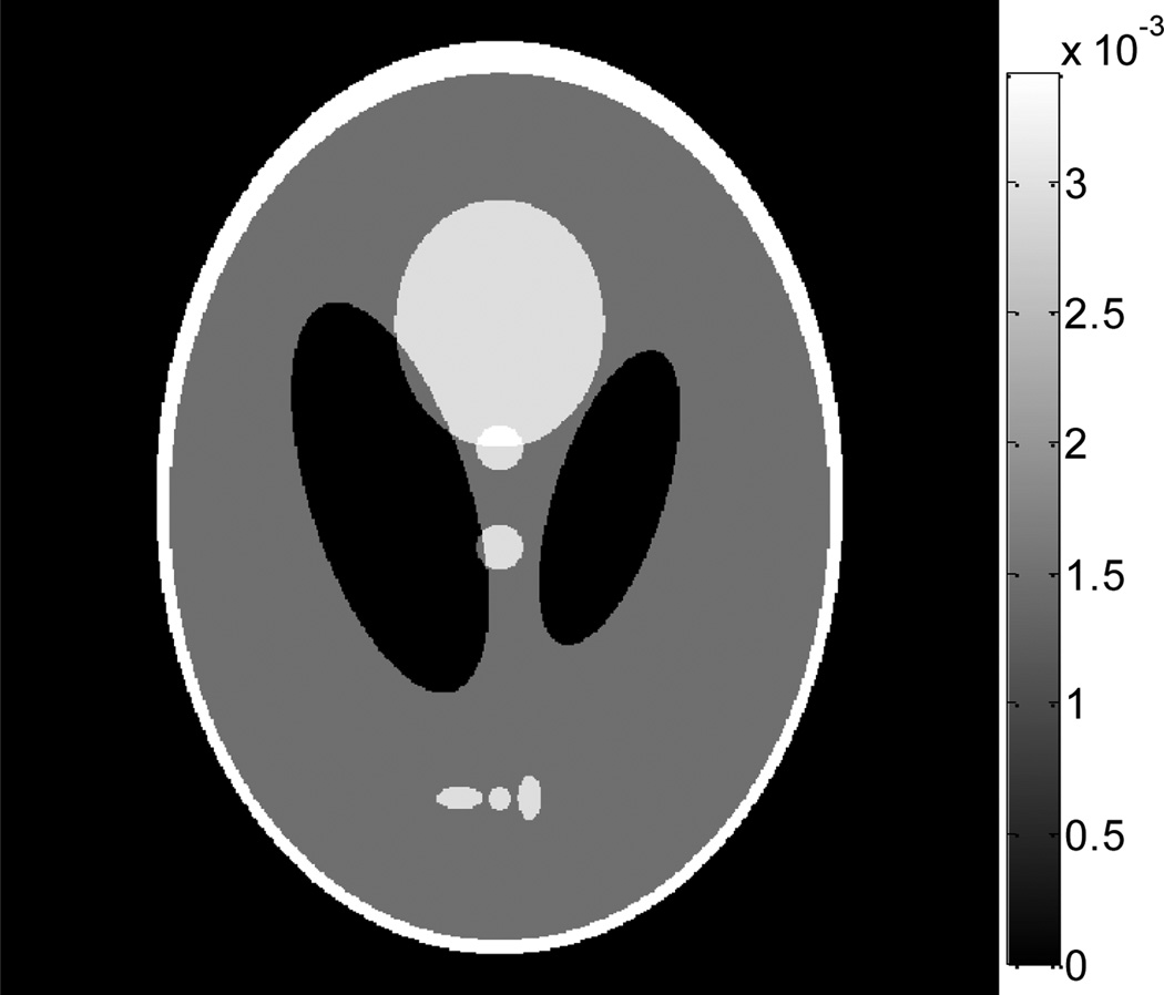
According to the mass attenuation coefficients as listed in Table 1 for different tissues at 80 KeV in [32], a modified Shepp-Logan phantom was carefully designed as shown in Fig. 1 for simulation studies. The dimensions of the phantom are 256×256mm2, consisting of 512×512 pixels.
Table 1.
Mass attenuation coefficients and the relate densities for different tissues.
| Body tissue | Mass attenuation coefficients μ/ρ (m2/kg) |
The density of tissue (kg/m3) in 20°C |
|---|---|---|
| Air, dry | 1.661×10⁻² | 1.205 |
| Water | 1.835×10⁻² | 1000 |
| Muscle | 1.822×10⁻² | 1040 |
| Fat | 1.805×10⁻² | 920 |
| Bone | 2.083×10⁻² | 1850 |
Figure 1.
A modified Shepp-Logan phantom with display window [0, 0.0034] mm−1.
With the parallel-beam imaging geometry, the noise-free sinogram can be computed by the line integration of the attenuation coefficients along the corresponding projection paths:
| (12) |
A set of noise-free sinograms was computed with 1024 detector bins per view and several different numbers of projection views, i.e., 20, 40 and 60, at equal angular increment on 360 degrees around the phantom.
3.1.2. Noise Model
Although the Compound Poisson model [33] is more accurate for description of the noise of the detected photon numbers in CT imaging, it is numerically challenging to implement this model for data noise simulation. Several reports have discussed the approximation of this model by the Poisson model [10, 11, 33, 34]. Based on these reports, the CT transmission data can be assumed to be a Poisson distributed quantum noise plus Gaussian distributed electronic noise [10, 35, 36]. In our simulation, we assumed that the detected photon number follows the Poisson process plus the electronic noise background [35, 36], in other words,
| (13) |
where Îi is the simulated noisy transmission datum and Ii is the mean number of photons or the noise-free transmission datum for detector bin i at a projection view, mic and are the mean and variance of the electronic noise, respectively, for detector bin i. By system calibration, the mean value is usually set to zero, mic = 0, and the variance was found in some clinical CT scanners [36].
Based on the noise model (13), the noisy transmission data can be simulated as follows. Given the modified mathematical Shepp-Logan phantom of Fig. 1, the line integral p̅i was computed along the projection path or ray i. By the Lambert-Beer’s law, ), and the knowledge of in routine clinical studies [9, 30 34, 36, 37], the mean Ii was calculated. Given the mean and a Poisson random number generator, the first term of Poisson (Ii) in (13) was obtained. The second term in (13) was obtained by the use of a Gaussian random number generator with zero mean and variance of 10. After the noisy transmission datum Îi was simulated from the noise-free transmission datum by sampling the Poisson variable with mean Ii and the Gaussian variable with mean of zero and variance of 10, the corresponding noisy projection datum pi was obtained by the logarithm transform of the noisy transmission datum:
| (14) |
3.1.3. Parameter Selection
To reconstruct the image of the Shepp-Logan phantom {μj} of Fig. 1 from the above simulated noisy sinogram data {pi}, we followed the description in [20, 21] to implement their TV-POCS algorithm. In a similar way to implement our AwTV-POCS algorithm, the parameter of δ in the weight of (5) shall be determined. By some experimental trials, the value of this scale factor was set to 0.6×10⁻² to simulate the strength of the diffusion model [25, 26]. For the EPTV-POCS method, the scale factor was also set to 0.6×10⁻² for comparison purpose. In addition to this parameter, another factor of ξ = 1.0×10⁻⁵ in (10) was set to ensure that the denominators will not go to zero. For the TV-POCS, EPTV-POCS and AwTV-POCS algorithms, each of the general iteration consisted of 10 POCS iterations and 10 gradient descent iterations. The strop criterion was discussed in Section 2.5 above. The error tolerance ε for the data constraint will be discussed later. The initial value of ω and τ were set as 1 and 0.7×10⁻⁵, respectively, similar to that in [20, 21].
3.1.4. Visualization-based Evaluation
In this evaluation study, two numerical experiments were performed: (1) image reconstruction from noise-free data; and (2) image reconstruction from noisy data. In each numerical experiment, images were reconstructed from the data simulated with 20, 40, 60 projection views, respectively, by the use of the AwTV-POCS algorithm with comparison to the TV-POCS and EPTV-POCS algorithms.
A. Noise-free Cases
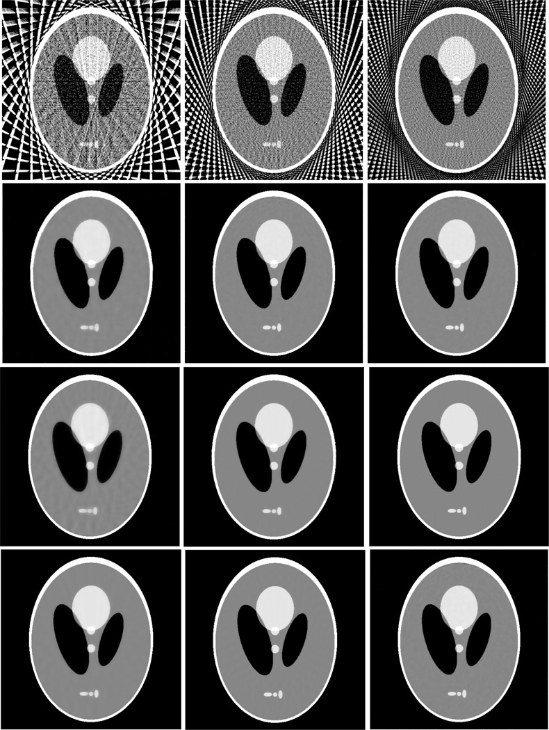
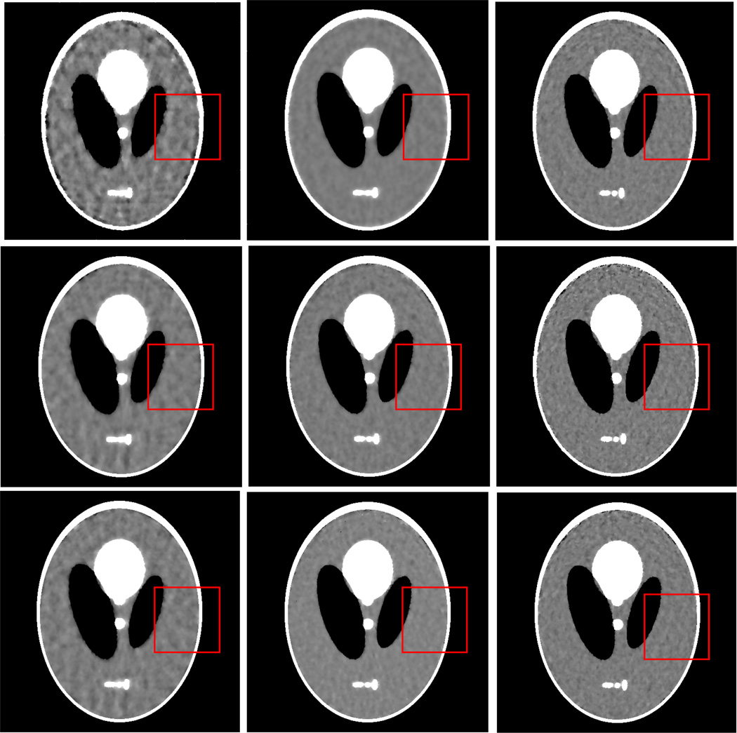
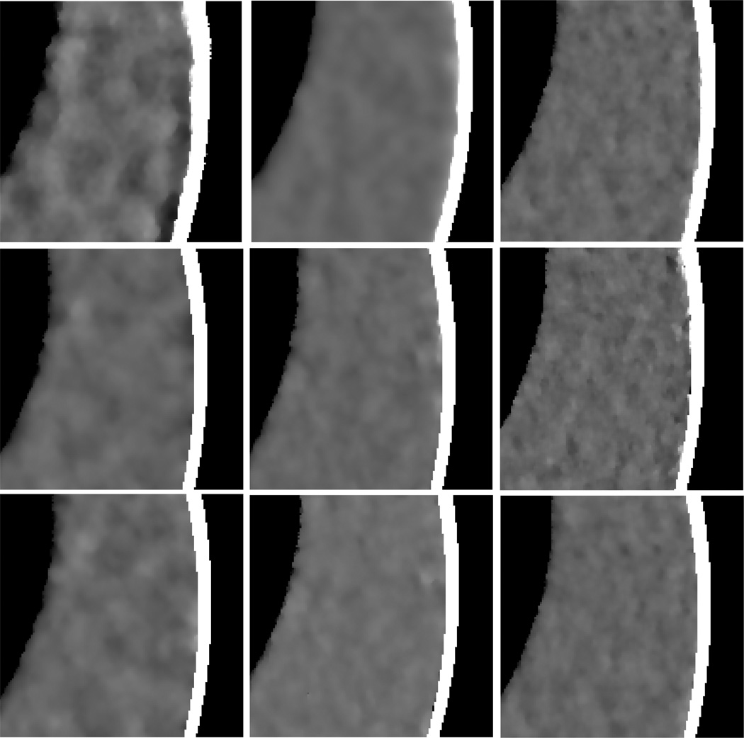
Figure 2 shows the results from the noise-free experiment. It can be observed that the images reconstructed by the TV-POCS, EPTV-POCS and AwTV-POCS are visually much better than the results of FBP in all the cases of 20, 40, 60 projection views. The difference between the images from the TV-POCS, EPTV-POCS and AwTV-POCS can be observed by using a narrow grayscale display window as shown in Fig. 3. Regions of interest (ROIs) in Fig. 3 were selected to examine some details of the reconstructed images. The corresponding ROIs results are shown in Fig. 4. It can be seen that, in the case of 20 projection views, the results of AwTV-POCS and EPTV-POCS algorithms demonstrate some gains in terms of edge preserving. Meanwhile, the gains gradually disappeared as more projection views were used. It is worth to note that a little over-enhancement at the edges in the EPTV-POCS reconstruction can be observed as shown in the second row of Fig.4, which is consistent with the results published in [23]. From 60 projection views, all the TV-POCS, EPTV-POCS and AwTV-POCS algorithms generated good quality images with high similarity.
Figure 2.
The images reconstructed by the FBP (1st row), TV-POCS (2nd row), EPTV-POCS (3rd row) and AwTV-POCS (4th row) algorithms from 20 (left column), 40 (middle column), and 60 (right column) projection views, respectively. The display window is [0, 0.0034] mm−1.
Figure 3.
The images reconstructed by the TV-POCS (top row), EPTV-POCS (middle row) and AwTV-POCS (bottom row) algorithms from 20 (left column), 40 (middle column), and 60 (right column) projection views, respectively. The display window is [0.0013, 0.0018] mm−1.
Figure 4.
The ROIs of the images reconstructed by the TV-POCS (top row), EPTV-POCS (middle row) and AwTV-POCS (bottom row) algorithms from 20 (left column), 40 (middle column), and 60 (right column) projection views, respectively. The display window is [0.0013, 0.0018] mm−1.
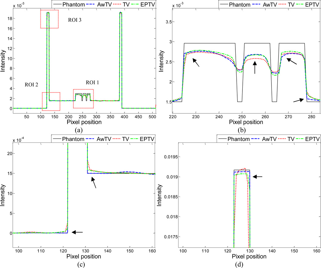
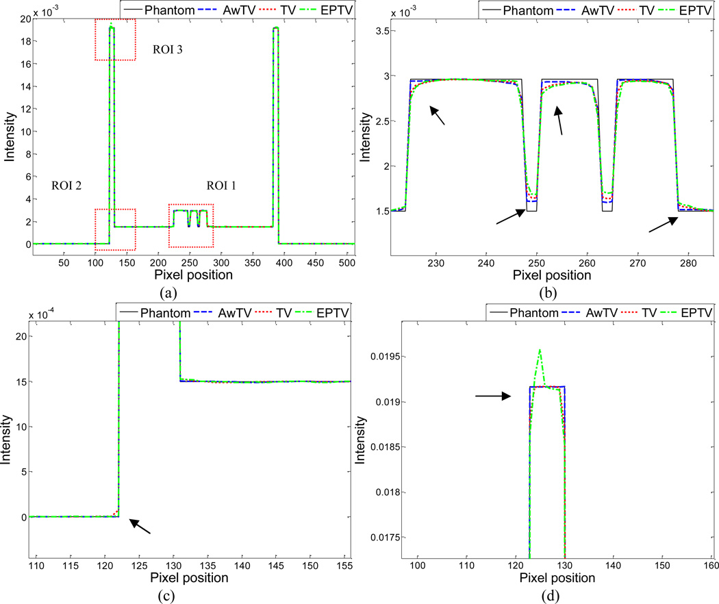
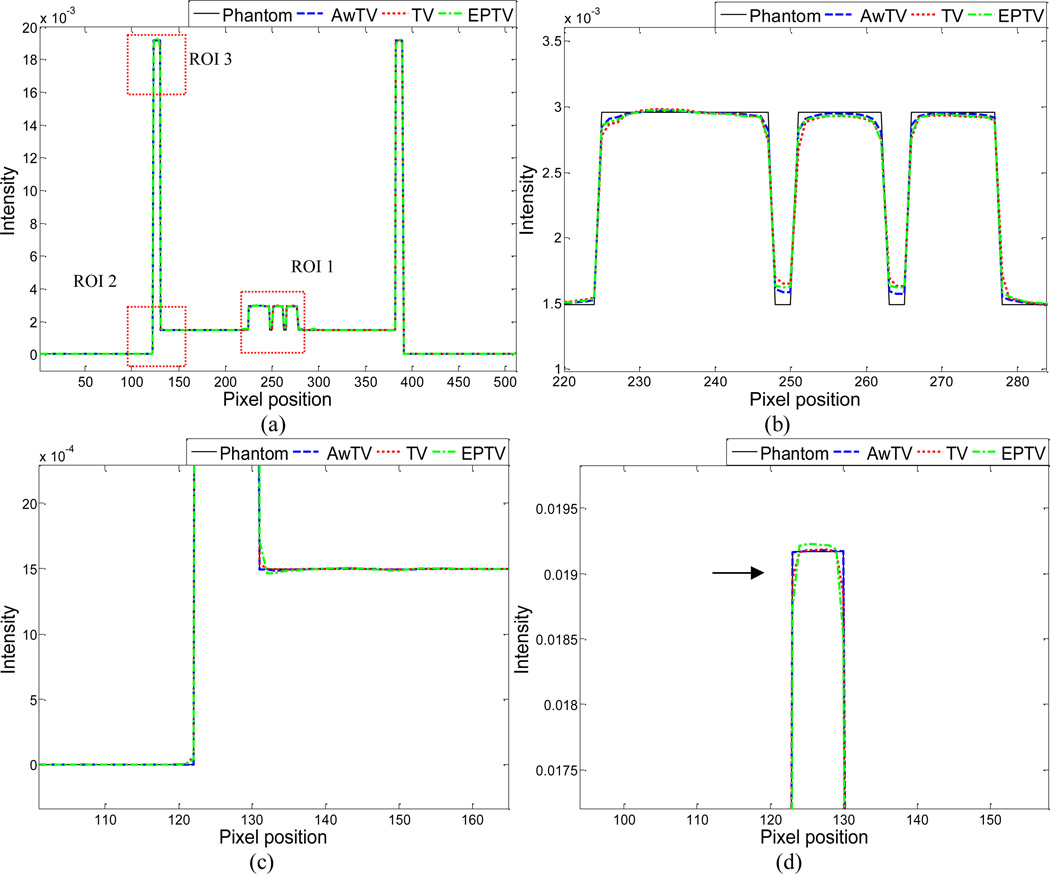
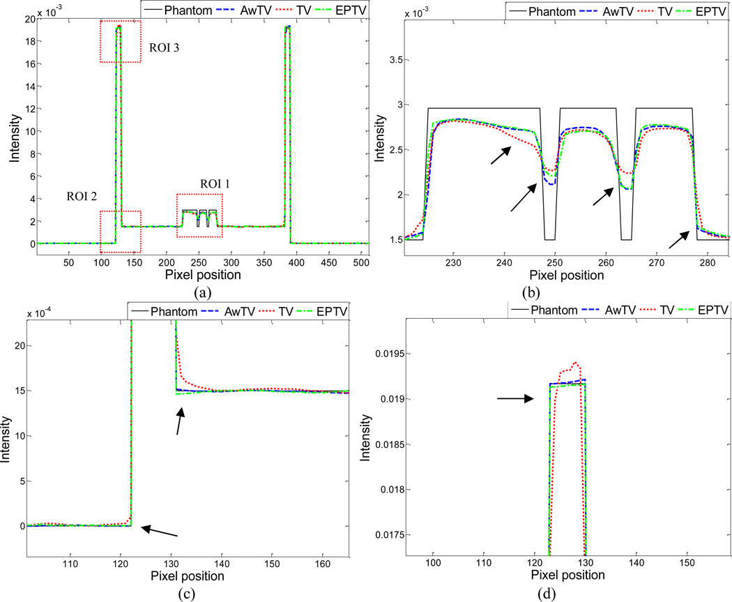
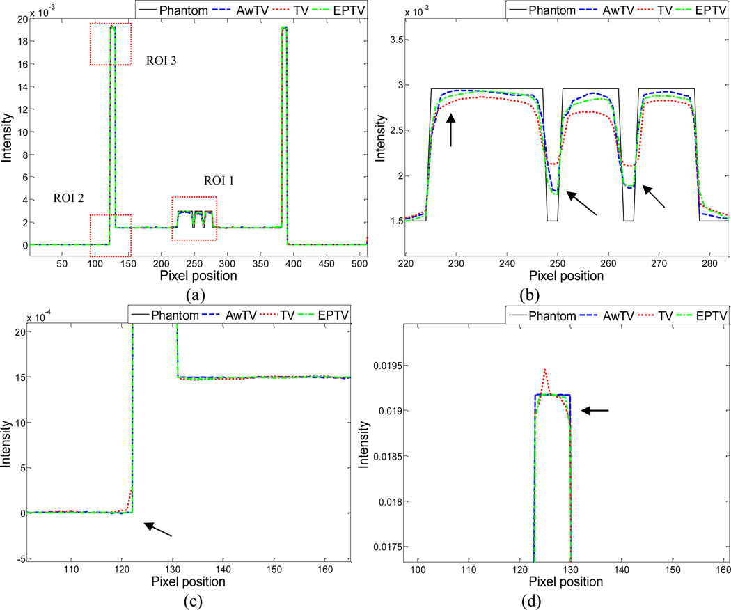
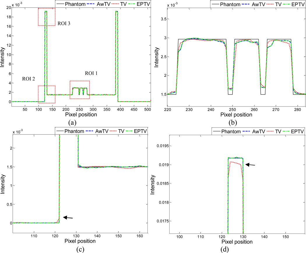
To further visualize the difference between the three approaches in the cases of 20, 40 and 60 projection views, horizontal profiles of the resulting images were drawn across the 410th row for each case and are shown in Figs. 5, 6 and 7, where the corresponding profile from the true phantom image is given for reference. In each case, three ROIs were selected to inspect the difference of the results. Figures 5(b)–(d) show that the AwTV-POCS and EPTV-POCS algorithms can achieve better profiles matching with the ideal ones than the TV-POCS algorithm. And the gain from the AwTV-POCS is observable as compared to results of the EPTV algorithm. As the number of projection views increased, the results of TV-POCS, EPTV-POCS and AwTV-POCS algorithms approached to that of the true phantom image. However, the improved edge preservation by the AwTV-POCS is still visible in the results from 60 projection views, see Fig. 7.
Figure 5.
Horizontal profiles (410th row) of the images reconstructed by different algorithms from 20 projection views of noise-free data. Picture (a) shows the overall profiles. Pictures (b), (c) and (d) show the partial profiles of the three ROIs indicated in (a).
Figure 6.
Horizontal profiles (410th row) of the images reconstructed by different algorithms from 40 projection views of noise-free data. Picture (a) shows the overall profiles. Pictures (b), (c) and (d) show the partial profiles of the three ROIs indicated in (a).
Figure 7.
Horizontal profiles (410th row) of the images reconstructed by different algorithms from 60 projection views of noise-free data. Picture (a) shows the overall profiles. Pictures (b), (c) and (d) show the partial profiles of the three ROIs indicated in (a).
The above noise-free simulation studies concurred with our previous discussion in Section 2.2 about the advantage of using adaptive weights for edge preservation in the AwTV model as compared to the conventional TV and EPTV models. To further support our previous discussion, studies on noisy projection data were performed and reported in the next section below.
B. Noisy Cases
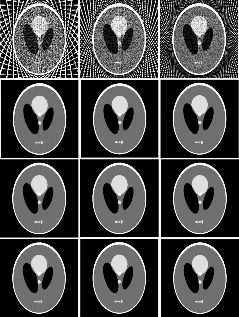
In this section, image reconstruction from noisy data was performed to analyze the robustness to noise of the AwTV-POCS algorithm. For all the AwTV-POCS, EPTV-POCS and TV-POCS algorithms, the value of the tolerance parameter ε were chosen to be 0.085, 0.082 and 0.078 for the 20, 40, and 60 projection views, respectively. A smaller ε value was chosen for a larger number of projection views byr the reason that the constraints in (1) and (3) would be more restrictive for more data samples. Figure 8 shows that the FBP images have noticeable artifacts as compared to the images reconstructed by the TV-POCS, EPTV-POCS and AwTV-POCS algorithms from 20, 40, and 60 projection views of the noisy sinogram data.
Figure 8.
The images reconstructed by the FBP (1st row), TV-POCS (2nd row), EPTV-POCS (3rd row) and AwTV-POCS (4th row) algorithms from 20 (left column), 40 (middle column), and 60 (right column) projection views of noisy sinogram data, respectively. The display window is [0, 0.0034] mm−1.
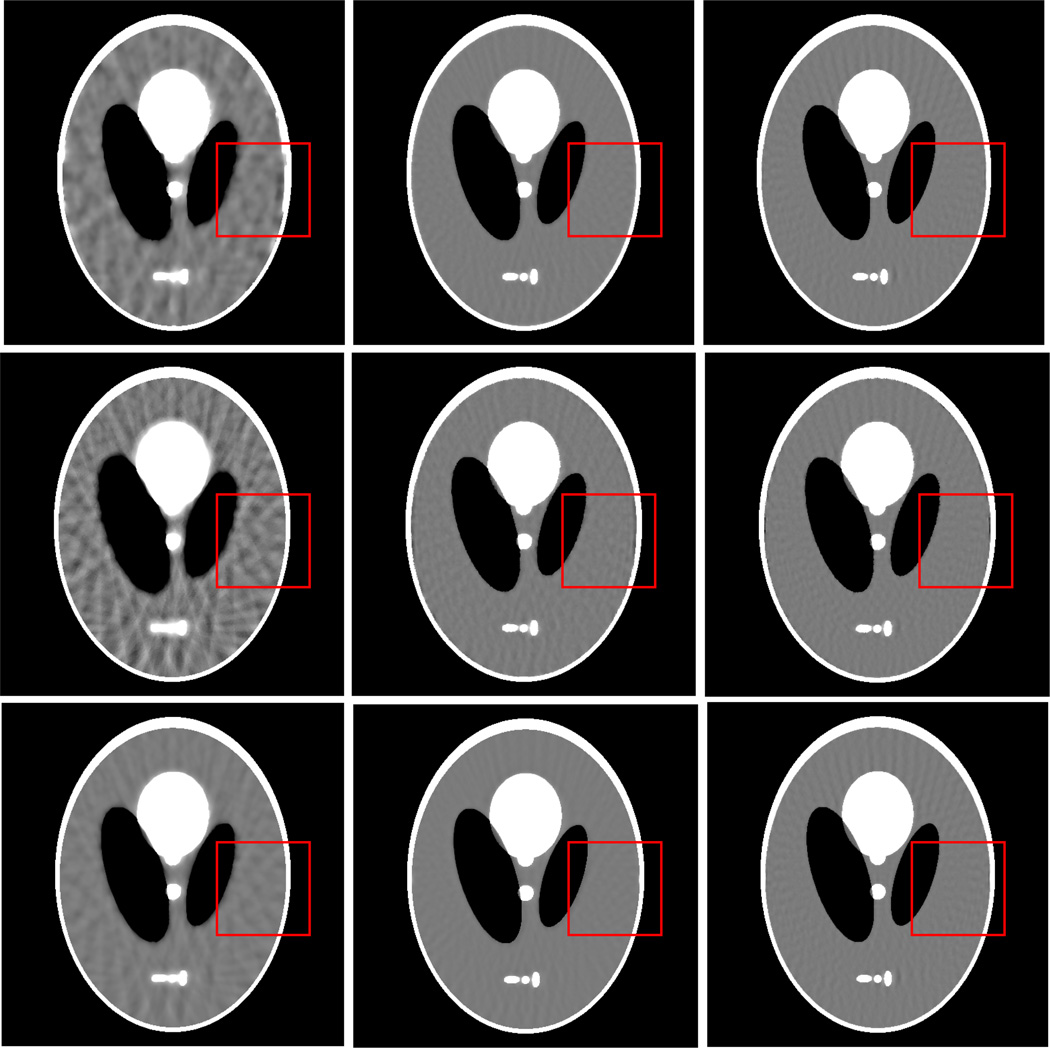
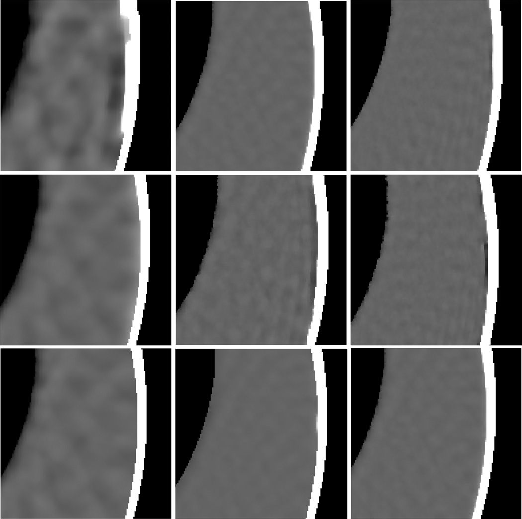
A narrow grayscale display window was presented to examine the differences among the results of the three latter approaches as shown in Figs. 9 and 10. Compared to the TV-POCS and EPTV-POCS algorithms, the AwTV-POCS algorithm preserved more edge details for 20 and 40 projection views and generated similar results for 60 projection views.
Figure 9.
The images reconstructed by the TV-POCS (top row), EPTV-POCS (middle row) and AwTV-POCS (bottom row) algorithms from 20 (left column), 40 (middle column), and 60 (right column) projection views of noisy sinogram data, respectively. The display window is [0.0013, 0.0018] mm−1.
Figure 10.
The ROIs of the images reconstructed by the TV-POCS (top row), EPTV-POCS (middle row) and AwTV-POCS (bottom row) algorithms from 20 (left column), 40 (middle column), and 60 (right column) projection views of noisy sinogram data, respectively. The display window is [0.0013, 0.0018] mm−1.
The horizontal profiles of the images reconstructed in the case of 20, 40 and 60 projection views of noisy data along the 410th row are shown in Figs. 11, 12 and 13, respectively, with the corresponding profile of the true phantom image as a reference. These profiles also show that the AwTV-POCS preserved the edge details better that the TV-POCS in the noisy case for 20, 40 and 60 projection views, except for the display of Fig. 13(b) which shows similar performance. The profiles also show that the results of AwTV-POCS and EPTV-POCS strategy is very close but some gains from the present AwTV-POCS can be observed as shown in Figs. 11(b)–(c)–(d) and Figs. 12(b)–(d). These noisy simulation studies were consistent with our previous observations in the noise-free cases, and further concurred with our previous discussion in Section 2.2 about the advantage of using the adaptive weights for edge preservation in the AwTV model as compared to the conventional TV model. With the same tendency as in the noise-free cases, the profiles in the noisy cases show that the reconstruction quality increased as the number of projection views increased. In the case of 60 projection views, the resulting images were closed to the true phantom image by all the TV-POCS, EPTV-POCS and AwTV-POCS approaches.
Figure 11.
Horizontal profiles (410th row) of the images reconstructed by different algorithms from 20 projection views of noisy data. Picture (a) shows the overall profiles. Pictures (b), (c) and (d) show the partial profiles of the three ROIs indicated in (a).
Figure 12.
Horizontal profiles (410th row) of the images reconstructed by different algorithms from 40 projection views of noisy data. Picture (a) shows the overall profiles. Pictures (b), (c) and (d) show the partial profiles of the three ROIs indicated in (a).
Figure 13.
Horizontal profiles (410th row) of the images reconstructed by different algorithms from 60 projection views of noisy data. Picture (a) shows the overall profiles. Pictures (b), (c) and (d) show the partial profiles of the three ROIs indicated in (a).
For the purpose of focusing on the edge characterization of the AwTV model, quantitative evaluation using observer detection power and computer simulation data is given in the Appendix of this paper.
3.2. Phantom Experiment Studies
To further realize the potential gain of the AwTV-POCS with comparison to the TV-POCS in more realistic cases, cone-beam data were acquired from two physical phantoms using a commercial CT scanner.
3.2.1 Experiment with the CatPhan® 600 Phantom
An image slice of the CatPhan® 600 phantom is shown in Fig. 14. Cone-beam CT projection data were acquired by an Acuity simulator (Varian Medical System, Palo Alto, CA) [26]. The X-ray tube current was set at 80 mA and the duration of the X-ray pulse at each projection view was set to be 12 ms. A total of 634 projection views were acquired for a fully 360-degree rotation on a circular orbit. The distance of source-to-axis is 100 cm and source-to-detector distance is 150 cm. The voxel size in the reconstructed image is 0.776×0.776×0.776 mm3. The array size of the reconstructed image is 350×350×8. Sparse projection datasets can be extracted from the total 634 projection views. For example, 63, 79, and 158 views, respectively, were extracted which are evenly distributed over 360 degrees. To ensure convergence to a stable solution, the parameter cα was set as −0.6 for AwTV-POCS algorithm and −0.5 for TV-POCS algorithm. Two POCS iterations and twelve gradient descent iterations were performed in each general loop. The execution time for each general iteration step was around 45 seconds on a HP PC with Intel Xeon X5450 CPU and 24 gigabyte memory. The 3D AwTV term was defined similarly as the 2D AwTV term and can be expressed as:
| (15) |
where z is the voxels’ index along the z-axis direction. By setting the weight as 1, the conventional TV term is obtained. The reconstructed images are shown in Figs. 14 and 15. The reconstruction by the well-known Feldkamp–Davis–Kress (FDK) method with Hanning window at Nyquist frequency cutoff is shown as reference image.
Figure 14.
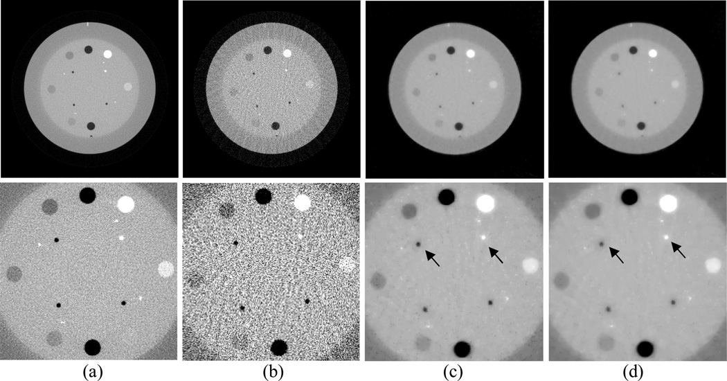
CatPhan® 600 phantom image reconstructions by different algorithms from 63 projection views. Column (a) shows the reconstruction by the FDK method from the total 634 projection views as a reference. Column (b) shows the reconstruction by the FDK algorithm from 63 projection views. Column (c) shows the reconstruction by the AwTV-POCS algorithm from 63 projection views. Column (d) shows the reconstruction by the TV-POCS algorithm from 63 projection views. The bottom row shows the zoomed pictures. The displokay window of top row is [0, 0.024]. The display window of bottom row is [0.008, 0.02] mm−1.
Figure 15.
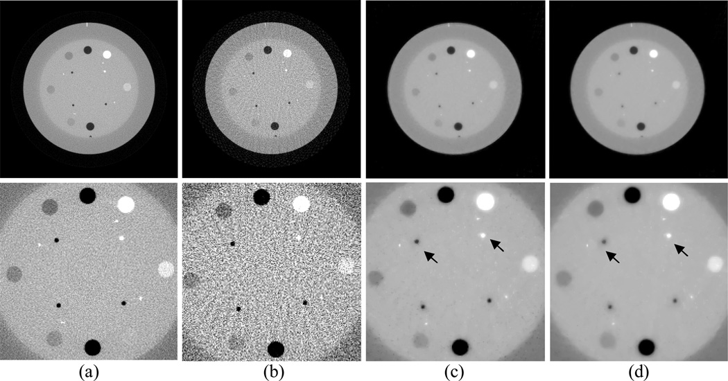
CatPhan® 600 phantom image reconstructions by different algorithms from 79 projection views. Column (a) shows the reconstruction by the FDK algorithm from the total 634 projection views as a reference. Column (b) shows the reconstruction by the FDK algorithm from 79 projection views. Column (c) shows the reconstruction by the AwTV-POCS algorithm from 79 projection views. Column (d) shows the reconstruction by the TV-POCS algorithm from 79 projection views. The bottom row shows the zoomed pictures. The display window of top row is [0, 0.024]. The display window of bottom row is [0.008, 0.02] mm−1.
From Fig. 14, it is seen that both the AwTV-POCS and TV-POCS algorithms reconstructed much better images as compared to the result of the FDK method from 63 projection views. In addition, the result of the AwTV-POCS shows more details on the edges than the result of the TV-POCS as indicated by the arrows in Figs. 14(c) and 14(d). As the number of projection views increased, the visually difference on the results of the AwTV-POCS and TV-POCS algorithms became not significant except for some small difference between the spots as indicated by the arrows in Figs. 15(c) and 15(d). This observation is consistent with our previous conclusion in the Shepp-Logan numerical phantom simulation study.
3.2.2. Experiment with the Anthropomorphic Head Phantom
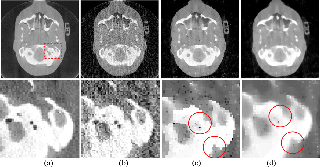
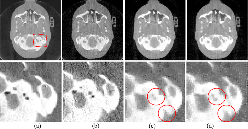
An image slice of the Anthropomorphic Head phantom is shown in Fig. 16. Cone-beam projection data were acquired from the anthropomorphic head phantom by the same protocol as used for the CatPhan® 600 phantom study. In order to observe the difference between the results from the AwTV-POCS and TV-POCS algorithms, we extracted 79 and 158 projection views from the full views for sparse image reconstruction. A ROI was selected to inspect the fine structures of the reconstructed results as indicated in Fig. 16(a). The resulting image and the ROI observations are shown in Figs. 16 and 17.
Figure 16.
Head phantom image reconstructions by different algorithms from 79 projection views. Column (a) shows the reconstruction by the FDK algorithm from the total 634 projection views as a reference. Column (b) shows the reconstruction by the FDK algorithm from 79 projection views. Column (c) shows the reconstruction by the AwTV-POCS algorithm from 79 projection views. Column (d) shows the reconstruction by the TV-POCS algorithm from 79 projection views. The bottom row shows the zoomed pictures. The display window is [0, 0.03]mm−1 for the first row and [0.01,0.03] mm−1 for the second row.
Figure 17.
Head phantom image reconstructions by different algorithms from 158 projection views. Column (a) shows the reconstruction by the FDK algorithm from the total 634 projection views as a reference. Column (b) shows the reconstruction by the FDK algorithm from 158 projection views. Column (c) shows the reconstruction by the AwTV-POCS algorithm from 158 projection views. Column (d) show the reconstruction by the TV-POCS algorithm from 158 projection views. The bottom row shows the zoomed pictures. The display window is [0, 0.03] mm−1 for the first row and [0.01,0.03] mm−1 for the second row.
By inspecting the images reconstructed from 79 projection views as shown in Fig. 16, it can be seen that some fine structures of the soft tissue, such as the structures of ear, are lost for both AwTV and TV models due to the sparse projection views. Despite this, some gains from the AwTV model are noticeable at both the ear location and the cold spots as indicated in the Figs. 16(b) and 16(c). By comparison to the CatPhan® 600 phantom result of Fig. 15, the loss of the fine structures in the results of head phantom as shown in Fig. 16 indicate that the measurements required for sparse image reconstruction should be associated with the structure of the signals. Intuitively, more projection views are needed to recover the fine structures in the head phantom. Based on this intuition, we performed another experiment by the use of 158 projections. Figure 17 shows the reconstructed results from the 158 projections. Significant improvement in recovering the small structures is seen by the use of more projections for both TV and AwTV models. The gain by the AwTV model is also noticeable as indicated by right lower circle in Figs. 17(c) and 17(d). These results are consistent with those from the Shepp-Logan phantom simulation study. This then suggests that the presented AwTV model can preserve the edge details better than the TV model for image reconstruction from sparse-viewed projections.
3.3. Quantitative Evaluation
In this section, two metrics for quantitative evaluation were used to show the performance of the AwTV-POCS algorithm with comparison to the TV-POCS algorithm.
3.3.1. Full Width at Half Maximum Measurement
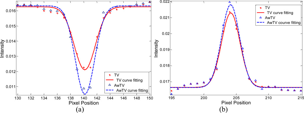
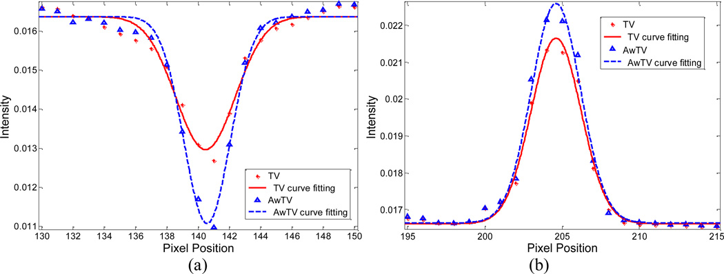
To quantitatively analyze the gain by using the AwTV model with comparison to the conventional TV model in the POCS framework, the full-width-at-half-maximum (FWHM) of two spots (a hot spot and a cold spot) of the CatPhan® 600 phantom as indicated in Figs. 14 and 15 are calculated. Figures 18 and 19 show the profiles passing through the two spots in the images reconstructed from 63 and 79 projection views, respectively. A Gaussian like function is used to fit the profiles as indicated in the figures, then the FWHM of the fitted Gaussian broadening kernel is calculated by 2.35σ. From Figs. 18 and 19, we can observe that the peak value of the result from the conventional TV-POCS algorithm is lower than that from the AwTV-POCS algorithm, which indicates that the AwTV-POCS algorithm can gain in resolution. The FWHM values of the reconstructions from 63 and 79 projection cases by TV-POCS and AwTV-POCS algorithms are shown in Table 2. Both of the cases reveal that the AwTV-POCS algorithm can produce a smaller FWHM value on both hot and cold spots compared to the TV-POCS strategy, which is consistent with our observation about the profile comparison.
Figure 18.
Horizontal profiles of the CatPhan® 600 phantom images reconstructed by different algorithms from 63 projection views of noisy data. Picture (a) shows the profiles across the cold spot (416th row, 130th to 150th column). Picture (b) shows the profiles across the hot spot (and 139th row, 195th to 215th column).
Figure 19.
Horizontal profiles of the CatPhan® 600 phantom images reconstructed by different algorithms from 79 projection views of noisy data. Picture (a) shows the profiles across the cold spot (416th row, 130th to 150th column). Picture (b) shows the profiles across the hot spot (and 139th row, 195th to 215th column).
Table 2.
The FWHM values of the cold and hot spots
| 63 Projection views | cold spot | hot spot |
| TV-POCS | 5.3580 | 4.7024 |
| AwTV-POCS | 4.8857 | 4.6690 |
| 79 Projection views | cold spot | hot spot |
| TV- POCS | 6.3168 | 5.3815 |
| AwTV-POCS | 4.8927 | 5.2922 |
3.3.2. Resolution-Noise Tradeoff Study on the AwTV Model
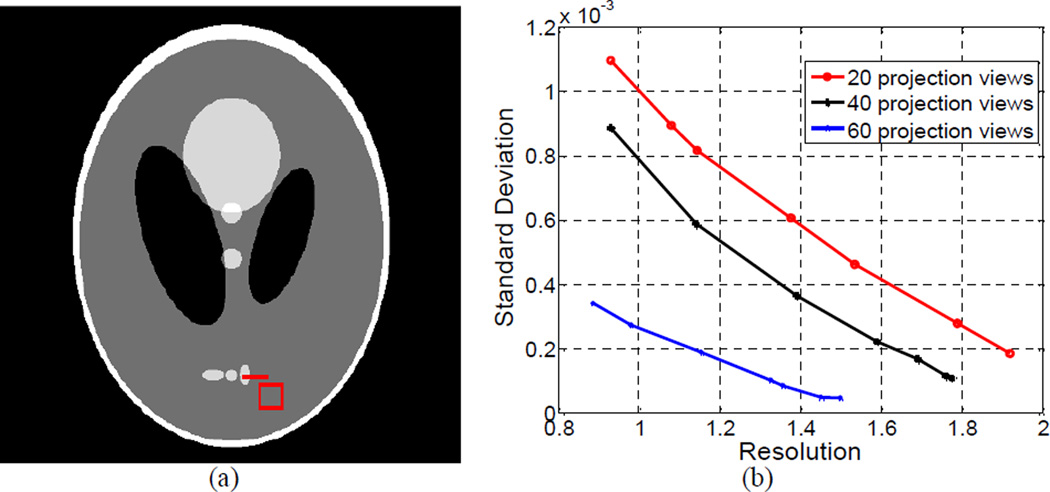
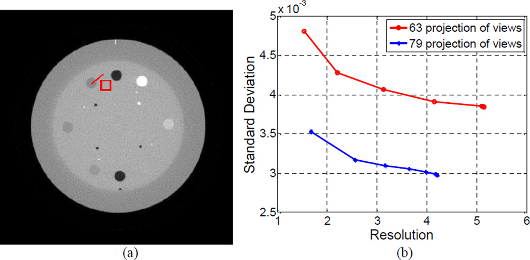
The parameter δ of the weight ws,s',t,t' in the AwTV model (5) plays an important role for the AwTV-POCS algorithm. Its effect on the image resolution and noise tradeoff was investigated in this study. The image resolution was calculated from the edge spread function (ESF) (a measurement of the broadening of a step edge) along the horizontal profile on the small vertical ellipse which is indicated at the right bottom of Fig. 20(a). The calculation procedure is based on the descriptions in [9, 10], where the edge broadening kernel is assumed as a Gaussian function with standard deviation σR, and an error function parameterized by σR is used to describe the ESF. By fitting a horizontal profile through the center of the small vertical ellipse to an error function, the parameter σR can be obtained. With the similar concept as introduced in previous section, the FWHM of the fitted Gaussian broadening kernel is calculated by 2.35σR, which indicates the resolution of the reconstructed image. In this study, the image noise was calculated from the pixels in a small square ROI, which was selected nearby the small vertical ellipse at the bottom right of Fig. 20(a). The standard deviation, σN, of the local uniform region in the ROI was used as the noise indicator. By varying the weight parameter δ from 0.3×10⁻² to 6.0, we can obtain a curve in the coordinates (σR, σN) Figure 20(b) shows three curves corresponding to the AwTV-POCS reconstructions from 20, 40, and 60 projection views, respectively. The resolution and noise tradeoff improved as the number of projection views increased. This observation concurs with the expectation in general sense, indicating the validity of the plots. For all the three cases of 20, 40, and 60 projection views, the standard deviation σN or noise measure of the reconstructed images decreased as δ increased, indicating that the images became “smoother”. In the meanwhile, the resolution measure σR of the reconstructed images also increased as δ increased, indicating that the edges became more “blurry”. This observation also concurs with the expectation in general sense, further indicating the validity of the plots. A similar evaluation was also performed using the reconstruction results from 63 and 79 projection views, respectively, of the CatPhan® 600 phantom. The corresponding resolution-noise tradeoff curve is shown in Fig. 21. Thus, according to the tendency of the resolution-noise tradeoff curves, it is possible to obtain an optimal resolution-noise tradeoff in the reconstruction by determining a proper value for δ. In all the simulation and experiment studies, a small value was used as the initial guess for the δ value. Staring from this small value, we increased the value empirically until a proper value δ was obtained, which rendered visual-appearing results. For example, δ = 0.6×10⁻² was found in the Shepp-Logan phantom cases, δ = 0.9×10⁻² in the CatPhan® 600 phantom cases, and δ = 0.01 in the anthropomorphic head phantom cases. Comparing to the TV-POCS reconstructions, the results from the AwTV-POCS algorithm did not show noticeable difference when δ >1.
Figure 20.
The resolution noise tradeoff curves from the Shepp-Logan phantom study. Picture (a) shows the modified Shepp-Logan phantom with display window [0, 0.0034] mm−1, where the square at the right bottom location is the selected ROI, the line on the right bottom small ellipse indicates the location of the profiles. Graph (b) shows the resolution-noise tradeoff curves from the reconstructed images using different values of δ for the 20, 40, and 60 projection views, respectively.
Figure 21.
The resolution noise tradeoff curves from the CatPhan® 600 phantom study. Picture (a) shows the CatPhan® 600 phantom with display window [0, 0.024] mm−1, where the square at the left top location is the selected ROI, the line on the left top small circle indicates the location of the profiles. Graph (b) shows the resolution-noise tradeoff curves from the reconstructed images using different values of δ for the 63 projection views.
3.4. Convergence Analysis
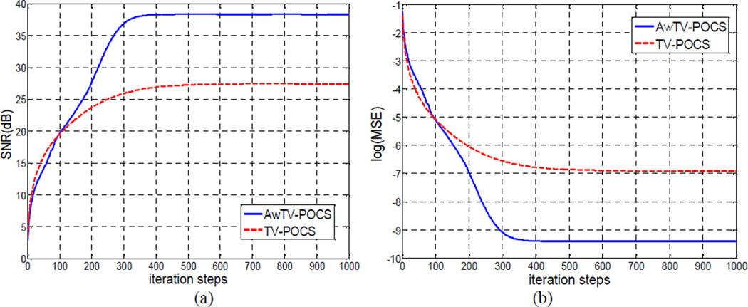
The signal-to-noise ratio (SNR) and mean-square-errors (MSE) metrics have been widely used to measure the noise level and image quality for a known signal, respectively. In this study, the convergence performance of the AwTV-POCS and TV-POCS algorithms was documented by calculating the SNR and the MSE versus the iteration steps. The definitions of SNR and MSE are listed as follows:
| (16) |
| (17) |
where μs,t is the true value of the attenuation coefficient at voxel location index (s, t) and μ̂s t is the reconstructed attenuation coefficient at voxel (s, t), M was defined before as the total number of image voxels. Each algorithm was executed up to 1,000 iteration steps to ensure its convergence to a stable solution.
Figure 22 shows the SNR and MSE versus the iteration steps for the AwTV-POCS and TV-POCS algorithms, respectively. Graphs 22(a) and 22(b) indicate that both the two algorithms converged robustly and reached their stable solutions after around 450 iterations. In addition to the SNR and MRE measures, the stop criterion cα of (11) was also considered. It dropped below −0.6 after 492 general iteration steps. As shown in Graph 22(a), the SNR of the AwTV-POCS reconstructions approached to 38dB at 1,000 iterations, as compared to the 27.5dB by the TV-POCS algorithm at the same number of iteration steps. This indicates that the AwTV-POCS algorithm can improve the SNR in reconstructions over the TV-POCS algorithm. From the curve of the MSE versus iteration steps, as shown in Graph 22(b), it can be observed that the reconstructions of the AwTV-POCS algorithm have a lower MSE level than that of the TV-POCS algorithm, indicating that the reconstructed images by the AwTV-POCS can be more accurate than the results of the TV-POCS algorithm.
Figure 22.
(a) -- SNR v.s. iteration steps. (b) -- log(MSE) v.s. iteration steps.
IV. Discussion and Conclusion
In this paper, we introduced a novel adaptive-weighted total variation (AwTV) minimization model for low-dose CT image reconstruction from sparse-view projection measurements. By introducing an anisotropic diffusion-based adaptive weight to preserve the edge information in the conventional TV minimization paradigm, the gain in mitigating the over-smoothing on the edges in the conventional TV minimization was observed by comparing the performance of the presented AwTV-POCS implementation with the established TV-POCS algorithm [20, 21].
In the computer simulation studies, the visual comparison via displaying the results of AwTV-POCS, EPTV-POCS and TV-POCS algorithms showed that the AwTV model enabled to reconstruct image satisfactorily without introducing artifacts from 20 projection views in both noise-free and noisy data cases compared to the conventional TV model and the EPTV model. Moreover, it should be noted that as the number of projection views increased to 40 and 60, all the algorithms improved the reconstruction quality compared to the results from 20 projection views. Similar tendency has also been observed in experiment studies (i.e., the CatPhan® 600 and anthropomorphic head phantoms). The reason is that a denser sampling of the data, by increasing the number of projection views, has stronger constraints to the sparse-view reconstruction optimization problem and, therefore, restricts the result much closer to the true image. This observation is consistent with the previous work of Bian et.al. [38]. In addition, more importantly, the present AwTV model can yield noticeable gain in preserving the fine structures and edges than the conventional TV model. In addition to the visual inspection, several more quantitative merits were utilized to analyze the differences between the presented AwTV and the conventional TV models. The following conclusions can be drawn from these quantitative measures.
Firstly, using the similar parameters for both TV and AwTV models (except parameter δ, which is only for the AwTV), the FWHM measure indicates that the results from the AwTV-POCS algorithm has higher peak and smaller values in both cold and hot spots as compared to the conventional TV-POCS algorithm. Thus, it could be concluded that the AwTV-POCS algorithm has a higher capability to preserve edge details compared to the conventional TV-POCS algorithm for sparse-view CT image reconstruction.
Secondly, the resolution-noise tradeoff study showed that the resolution in AwTV-POCS reconstructed images decreases with increasing the value of scale parameter δ. In the meanwhile, the standard deviation of image noise decreases. This observation indicates that a smoother image is obtained with a larger δ value. On the contrary, while decreasing the δ, the resolution and noise level increased, indicating a sharper image being obtained. Based on this observation, it could be concluded that the weight in AwTV model for edge information can give an optimal image quality by a proper value of δ, and the determination of this proper value is currently empirical.
Except the above quantitative measurements, the ROC study using the Shepp-Logan phantom (as shown in Appendix A) indicated that both TV-POCS and AwTV-POCA algorithms have similar detection performances when the small lesion’s contrast is too low or too high. In the former case both algorithms would certainly fail, while in the later case both algorithms would certainly succeed. However, when the small lesion contrast is in the between, the values of the AUC (area under the curve) of the receiver operating characteristics (ROC) of the AwTV-POCS are statistically significantly higher than that of the TV-POCS. In addition, the bias-variance tradeoff study (as shown in Appendix B) indicated that both algorithms have smaller bias and variance values at lower noise levels and their values are very close when the noise level is very low. However, at the same variance level, the AwTV-POCS has less bias than the TV-POCS. Although both the results from the ROC study and bias-variance analysis indicated that the AwTV-POCS algorithm can have higher quantitative capability in its reconstructions than the TV-POCS algorithm, it should be mentioned that more studies should be conducted by using more realistic clinical data than the simulated Shepp-Logan phantom data. For this reason, both the ROC and bias-variance results are presented in the Appendix.
Lastly but not the least, the convergence study showed that both TV-POCS and AwTV-POCS algorithms converged to their stable solutions, respectively, and had similar convergence rates, see Fig. 22. The converged solution of the AwTV-POCS had higher SNR and less MSE than that of the TV-POCS. Thus, it could be concluded that the AwTV-POCS can reconstruct more accurate images than the TV-POCS.
Based on both the qualitative inspection and quantitative measure of the reconstructions from the AwTV-POCS and TV-POCS algorithms, the gain by incorporating the edge characteristics into the AwTV model is noticeable. The gain shall be attributed to the AwTV model because both algorithms were implemented similarly in data constraints and numerical calculations, except for the TV and AwTV terms. Thus, it could be conjectured that the AwTV model can gain in different implementations in the case of both the parallel-beam projection geometry and nonparallel-beam projection geometries. In practice, the presented AwTV model can further incorporate different data constraints with associated optimization strategies for different applications. One typical example is to add data statistics into the cost function for penalized likelihood image reconstruction [39, 40], which will be an interesting topic for further research. In addition, the comparison between the AwTV model and EPTV model by using clinical data are also interested for further research. Besides the model analysis, many novel methods have been proposed to accelerate the convergence for solving similar inverse problems with TV regularization, such as the gradient-projection-Barzilai-Borwen method [41], the accelerated barrier optimization compressed sensing method [42] and the Unknown-Parameter Nesterov method [43]. The common idea of these methods is using the single-step gradient calculation to solve the TV regularization problem instead of using the presented two-step alternative optimization scheme. Compared with the TV-POCS and AwTV-POCS algorithms, the single-step method can fast converge to the optimal solution without reducing image quality. However, the step-size of the gradient calculation should be carefully designed to balance the convergence speed and accuracy. For example, the well known “line-search” scheme could guarantees the monotonic convergence, but it may need an intensive computation. In contrary, although a fixed large step-length in the conventional gradient scheme can reduce the computing burden, the outcome could be unacceptable. Thus, proper strategies for parameter estimation are necessary when designing a new algorithm [41, 43]. To apply the proposed AwTV model to clinical data, where the image size is always large because of the need of high resolution, a new algorithm with less computation complexity would be always desired for our further research.
Acknowledgement
This work was partially supported by the NIH/NCI under grants #CA143111 and #CA082402. J. Ma also was partially supported by the NSF of China under grants #81000613 and #81101046 and the National Key Technologies R&D Program of China under grant #2011BAI12B03. The comments on the scientific aspects and the assistance of providing the cone-beam phantom data for evaluation studies of this work from Dr. Jing Wang shall be acknowledged.
Appendix A
(Receiver Operating Characteristic Study)
One of the important tasks for medical image analysis is helping the physicians to detect lesions or abnormalities. The receiver operating characteristic (ROC) curve, which plots the tradeoff between the true-positive (TP) and true-negative scores, is extensively used as a valuable merit to evaluate the diagnostic accuracy for a medical imaging system and/or image reconstruction algorithm. In practice, the ROC curve can be generated by the pairs of the TP fraction and false positive fraction [9, 44] with different confidence thresholds. The most common measure for comparison of the ROC curves is the area under the curve (AUC). An image reconstruction algorithm, which generates a larger AUC, usually has a higher capability for detection of abnormalities.
Human observer is one of the most desired observers, but the procedure needs an experienced physician to manually evaluate each case, which is time consuming for processing a large number of cases. The channelized hotelling observer (CHO) is one of the most efficient numerical observers that can help us to evaluate the algorithms without performing the human observer procedure. In our studies, we utilized the four octave-wide rotationally symmetric frequency channels proposed by Myers and Barrett [45], which have been shown to give good predictions of a human observer procedure in abnormal detection. In our implementation of the CHO procedure, each reconstructed image generated a four-element feature vector according to the four channels, and the CHO was trained for the AwTV-POCS and TV-POCS algorithms, respectively. A group of scalar rating values were produced from different independent ensemble of the feature vectors of the reconstructed images in two class of categories (i.e., with or without lesion) by using the CHO_MAT code [46]. The scores were subsequently analyzed using the ROCKIT [44] and the AUC values were calculated to document the detection efficiency.
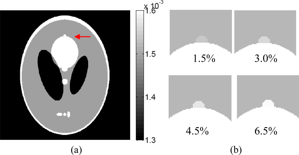
Since a large sample size is needed to perform the ROC study, computer simulation is usually the choice. For the detection task, a low contrast small lesion of radius 3 mm was simulated as a growth from the big ellipse in the Shepp-Logan phantom as shown in Fig. 23, where the arrow indicates the lesion. Four intensity contrast levels of the added lesion were considered as 1.5%, 3.0%, 4.5% and 6.5%, respectively, higher than that of the background to evaluate the performance of detection efficiency for the two reconstruction algorithms, i.e., TV-POCS and AwTV-POCS.
Figure 23.
(a) shows the modified Shepp-Logan phantom used for the ROC studies, where the display window is [0.0013, 0.0016]. (b) shows the lesion at 1.5%, 3.0%, 4.5%, and 6.5% contrast levels, respectively, where the display window is [0.0013, 0.0016] mm−1.
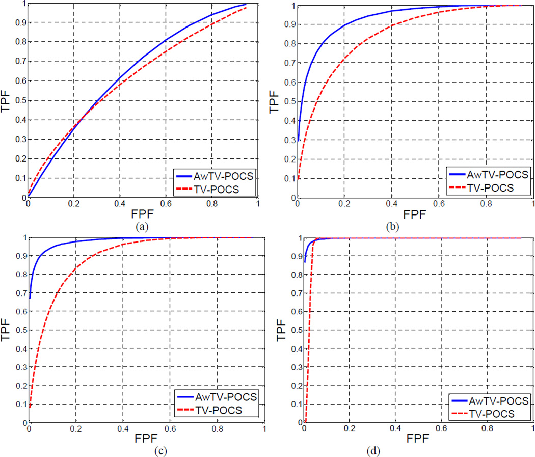
Noise-free projections from the Shepp-Logan phantom of Fig. 23(a) without and with the lesion at each lesion contrast level of Fig. 23(b) were first computed as described in Section 3.1.1 above. A total of five sets of noise-free data were computed. One set has no lesion and the other four sets have the lesion with the four different contrast levels in Fig. 23(b). From each noise-free dataset, a total of 500 noisy realizations were generated using the noise model of Section 3.1.2 above. These noisy sinogram data were then reconstructed by the two algorithms of TV-POCS and AwTV-POCS, respectively. A ROI of 19×19 pixel array size on each reconstructed image was selected around the lesion structure as the input of the CHO_MAT code. The series of ratings from the CHO output were subsequently analyzed using the ROCKIT package with bi-normal model. For each contrast level of the lesion, the ROC curves obtained from the two algorithms are shown in Fig. 24, and the AUC values are listed in Table 3.
Figure 24.
The ROC curves of the two algorithms: AwTV-POCS and TV-POCS. Graph (a) shows the ROCs for the lesion with 1.5% contrast level. Graph (b) shows the ROCs for the lesion with 3% contrast level. Graph (c) shows the ROCs for the lesion with 4.5% contrast level. Graph (d) shows the ROCs for the lesion with 4.5% contrast level.
Table 3.
The AUC measures and the one-tailed P-values for different lesion contrast levels from the AwTV-POCS and TV-POCS reconstructions. Note N/A in the right lower corner indicates that the value could not be obtained by the ROCKIT package.
| Lesion’s Intensity | AwTV-POCS (AUC) | TV-POCS (AUC) | One-tailed P-value |
|---|---|---|---|
| 1.5% | 0.6496 | 0.6264 | 0.3473 |
| 3.0% | 0.9301 | 0.8460 | 0.0089 |
| 4.5% | 0.9796 | 0.8940 | 0.0033 |
| 6.5% | 0.9964 | 0.9711 | N/A |
From Fig. 24 and Table 3, it can be seen that at 1.5% level, the AUC value from the AwTV-POCS was 0.6496 and from the TV-POCS was 0.6264. The one-tailed p-value was 0.3473 (greater than 0.05), which indicates that the difference between the two algorithms are not statistically significant at the 1.5% contrast level. In other words, both algorithms could not be able to detect the low-contrast lesion effectively. At the higher contrast levels of 3.0% and 4.5%, the AUC value from the AwTV-POCS was 0.9301 and 0.9796, respectively, whereas 0.846 and 0.894 from the TV-POCS. The one tailed p-value of the two algorithms was 0.0089 and 0.0039, respectively, which are less than 0.05, indicating the difference between these two algorithms is statistically significant at the 3% and 4.5% contrast levels. In other words, the AwTV-POCS can outperform the TV-POCS for the lesion contrast levels at 3.0% and 4.5%. To get further insight into these two algorithm, we considered the next higher contrast level of 6.5%. At this level, the AUC value of the AwTV-POCS algorithm reached 0.9964, indicating a perfect detection performance; and the value of the TV-POCS algorithm is slightly smaller, i.e., 0.9711. At such high contrast level, both algorithms can detect the lesion successfully, and it is expected that they shall perform similarly.
From the above ROC studies for different lesion contrast levels, it can be observed that the AwTV-POCS can outperform the TV-POCS in detecting small low contrast lesions because of the modeling of edge properties in the AwTV model. It is expected that both algorithms will perform similarly if the lesion contrast level is too low where both will surely fail, and too high where both will surely succeed. Although the results indicated that the AwTV-POCS has advantages compared to the TV-POCS strategy, more experiments using clinical data are needed in further studies.
Appendix B
(Bias v.s. Variance Tradeoff)
Another common merit for imaging system evaluation is the bias v.s. variance tradeoff plot, which is also one of the general figures of merit for evaluating the quality of reconstructed images. The plot describes the strength of the signal in relationship to the quantity of noise.
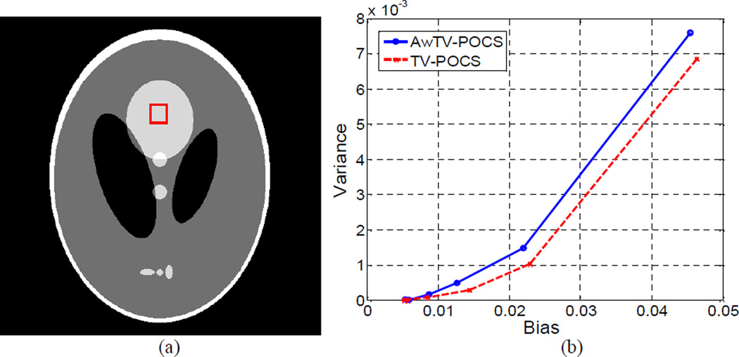
In this study, we focused on the robustness to different noise levels of the two algorithms in their reconstructions from the 20 projection views, where these two algorithms showed noticeable difference in the computer simulation studies, see Section 2.1 above. A ROI of 19×19 array size on the uniform image intensity was selected inside the top middle ellipse, as indicated in Fig. 25(a). Six different values of from 5.0×10³ to 2.5×10⁶ were selected to simulate noisy data at the corresponding noise levels. At each noise level, 100 noisy data samples were simulated and their reconstructions were performed by the use of the two algorithms, respectively. These reconstructions were then used to calculate the bias and variance. According to the description in [47, 48], the bias and variance are expressed as follows:
| (B1) |
| (B2) |
where μs,t is the true value of the attenuation coefficient at voxel location index (s, t), μ̂s,t is the reconstructed attenuation coefficient at voxel (s, t), and is the sample mean from the 100 samples of the resulting images at voxel (s, t). The over bar in (B1) and (B2) denotes the mean over the 100 noise realization samples. W is the pixel’s indices within the ROI and MW is the number of voxels in the ROI.
Figure 25.
The bias-variance plots. Picture (a) shows the modified Shepp-Logan phantom with display window [0, 0.0034] mm−1, where a rectangle ROI in the top middle ellipse is selected. Graph (b) shows the bias-variance curves for different noise levels.
Figure 25(b) shows the bias-variance plots of the AwTV-POCS and TV-POCS algorithms. Both algorithms can yield very small bias and variance values at low noise level (approaching to the origin of the plot), indicating that they can reconstruct high quality images at low noise level for the sparse-signal Shepp-Logan phantom with 20 projection views. When the noise level went up as the incident photon number went down below , some difference between these two algorithms were observed. This observation concurs with the simulation results in Section 3.1, indicating the validity of the plots. At the same variance or the same noise level, the images reconstructed by the AwTV-POCS have less bias as compared to the results of the TV-POCS. In other words, the AwTV-POCS can outperform the TV-POCS in terms of the bias-variance plots.
References
- 1.Brenner DJ, Hall EJ. CT--an increasing source of radiation exposure. New England Journal of Medicine. 2007 Nov;vol. 357:2277–2284. doi: 10.1056/NEJMra072149. [DOI] [PubMed] [Google Scholar]
- 2.Einstein AJ, Henzlova MJ, Rajagopalan S. Estimating risk of cancer associated with radiation exposure from 64-slice CT coronary angiography. Journal of American Medical Association. 2007 Jul;vol. 298:317–323. doi: 10.1001/jama.298.3.317. [DOI] [PubMed] [Google Scholar]
- 3.Kalra MK, Wittram C, Maher MM, Sharma A, Avinash GB, Karau K, Halpern TL, Saini S, Shepard JA. Can noise reduction filters improve low-radiation-dose chest CT images? Pilot study. Radiology. 2003 Jul;vol. 228(1):257–264. doi: 10.1148/radiol.2281020606. [DOI] [PubMed] [Google Scholar]
- 4.Smith A, Dillon W, Gould R, Wintermark M. Radiation dose-reduction strategies for neuroradiology CT protocols. American Journal of Neuroradiology. 2007 Oct;vol. 28(9):1628–1632. doi: 10.3174/ajnr.A0814. [DOI] [PMC free article] [PubMed] [Google Scholar]
- 5.McCollough CH, Primak AN, Braun N, Kofler J, Yu L, Christner J. Strategies for reducing radiation dose in CT. Radiologic Clinics of North America. 2009 Jan;vol. 47(1):27–40. doi: 10.1016/j.rcl.2008.10.006. [DOI] [PMC free article] [PubMed] [Google Scholar]
- 6.Li X, Orchard MT. Spatially adaptive image de-noising under over-complete expansion. Conference Proceeding of IEEE Image Processing 2000. 2000 Sep;vol. 3:300–303. [Google Scholar]
- 7.Lu H, Hsiao I, Li X, Liang Z. Noise properties of low-dose CT projections and noise treatment by scale transformations. Nuclear Science Symposium and Medical Imaging Conference Record. 2001 Nov;vol. 3:1662–1666. [Google Scholar]
- 8.Li T, Li X, Wang J, Wen J, Lu H, Hsieh J, Liang Z. Nonlinear sinogram smoothing for low-dose X-ray CT. IEEE Transactions on Nuclear Science. 2004 Oct;vol. 51(no. 5):2505–2513. [Google Scholar]
- 9.Wang J, Li T, Lu H, Liang Z. Penalized weighted least-squares approach to sinogram noise reduction and image reconstruction for low-dose X-ray CT. IEEE Transactions on Medical Imaging. 2006 Oct;vol.25(10):1272–1283. doi: 10.1109/42.896783. [DOI] [PMC free article] [PubMed] [Google Scholar]
- 10.La Rivière PJ, Bian J, Vargas PA. Penalized-likelihood sinogram restoration for CT. IEEE Transactions on Medical Imaging. 2006 Aug;vol. 25(8):1022–1036. doi: 10.1109/tmi.2006.875429. [DOI] [PubMed] [Google Scholar]
- 11.Elbakri IA, Fessler JA. Statistical image reconstruction for polyenergetic X-ray CT. IEEE Transaction on Medical Imaging. 2002 Feb;vol. 21(2):89–99. doi: 10.1109/42.993128. [DOI] [PubMed] [Google Scholar]
- 12.Elbakri IA, Fessler JA. Efficient and accurate likelihood for iterative image reconstruction in X-ray CT. Proceeding of SPIE Medical Imaging, 2003. 2003 Feb;vol. 5032:1839–1850. [Google Scholar]
- 13.Donoho D. Compressed sensing. IEEE Transactions on Information Theory. 2006 Apr;vol. 52(4):1289–1306. [Google Scholar]
- 14.Candès E, Wakin M. An introduction to compressive sampling. IEEE Signal Processing Magazine. 2008 Mar;:21–30. [Google Scholar]
- 15.Candès E, Romberg J, Tao T. Robust uncertainty principles: Exact signal reconstruction from highly incomplete frequency information. IEEE Transactions on Information Theory. 2006 Feb;vol. 52(2):489–509. [Google Scholar]
- 16.Chen G, Tang J, Leng S. Prior image constrained compressed sensing (PICCS) Proc. Soc. Photon Instrum. Eng. 2008 Mar;vol. 6856:1–18. doi: 10.1117/12.770532. [DOI] [PMC free article] [PubMed] [Google Scholar]
- 17.Ma J, Huang J, Feng Q, Zhang H, Lu H, Liang Z, Chen W. Low-dose computed tomography image restoration using previous normal-dose scan. Medical Physics. 2011 Oct;vol. 38:5714–5731. doi: 10.1118/1.3638125. [DOI] [PMC free article] [PubMed] [Google Scholar]
- 18.Xu Q, Yu H, Mou X, Zhang L, Hsieh J, Wang G. Low-Dose X-ray CT Reconstruction via Dictionary learning. IEEE Transactionson Medical Imaging. 2012 Sep;vol.31(9):1682–1697. doi: 10.1109/TMI.2012.2195669. [DOI] [PMC free article] [PubMed] [Google Scholar]
- 19.Liu Y, Ma J, Fan Y, Liang Z. An investigation on CT image reconstruction with compressed sensing by l1 norm prior image constraints; Nuclear Science Symposium and Medical Imaging Conference Record; 2011. Nov, in CD-ROM. [Google Scholar]
- 20.Sidky E, Kao C, Pan X. Accurate image reconstruction from few-views and limited angle data in divergent-beam CT. Journal of X-Ray Science and Technology. 2006;vol. 14(2):119–139. [Google Scholar]
- 21.Sidky E, Pan X. Image reconstruction in circular cone-beam CT by constrained, total-variation minimization. Physics in Medicine and Biology. 2008 Aug;vol. 53:4777–4807. doi: 10.1088/0031-9155/53/17/021. [DOI] [PMC free article] [PubMed] [Google Scholar]
- 22.Ruding LI, Osher S, Fatemi E. Nonlinear total variation based noise removal algorithms. Physica D. 1992 Nov;vol. 60(1–4):259–268. [Google Scholar]
- 23.Tian Z, Jia X, Yuan K, Pan T, Jiang S. Low-dose CT reconstruction via edge-preserving total variation regularization. Physics in Medicine and Biology. 2011 Sep;vol. 56:5949–5967. doi: 10.1088/0031-9155/56/18/011. [DOI] [PMC free article] [PubMed] [Google Scholar]
- 24.Joseph PM. An improved algorithm for reprojecting rays through pixel images. IEEE Transactions on Medical Imaging. 1982 Nov;vol. 1(3):192–196. doi: 10.1109/TMI.1982.4307572. [DOI] [PubMed] [Google Scholar]
- 25.Perona P, Malik J. Scale-space and edge-detection using anisotropic diffusion. IEEE Transactions on Pattern Analysis and Machine Intelligence. 1990 Jul;vol. 12(7):629–639. [Google Scholar]
- 26.Wang J, Li T, Liang Z, Xing L. Dose reduction for kilovotage cone-beam CT in radiation therapy. Physics in Medicine and Biology. 2008 May;vol. 53:2897–2909. doi: 10.1088/0031-9155/53/11/009. [DOI] [PubMed] [Google Scholar]
- 27.Andersen A, Kak A. Simultaneous algebraic reconstruction technique (SART): A superior implementation of ART. Ultrasonic Imaging. 1984 Jan;vol. 6(1):81–94. doi: 10.1177/016173468400600107. [DOI] [PubMed] [Google Scholar]
- 28.Jiang M, Wang G. Convergence of the simultaneous algebraic reconstruction technique (SART) Conference Record of the Thirty-Fifth Asilomar Conference on Signal, Systems and Computers 2011. 2001 Nov;vol. 1:360–364. [Google Scholar]
- 29.Penfold S, Schulte R, Censor Y, Rosenfeld A. Total variation superiorization schemes in proton CT image reconstruction. Medical Physics. 2010 Oct;vol. 37:5887–5895. doi: 10.1118/1.3504603. [DOI] [PMC free article] [PubMed] [Google Scholar]
- 30.Dfrise M, Vanhove C, Liu X. An algorithm for total variation regularization in high-dimensional linear problems. Inverse Problem. 2011 May;vol. 6:065002. [Google Scholar]
- 31.Ma J, Feng Q, Feng Y, Huang J, Chen W. Generalized Gibbs priors based positron emission tomography reconstruction. Computers in Biology and Medicine. 2010 May;vol. 40(6):565–571. doi: 10.1016/j.compbiomed.2010.03.012. [DOI] [PubMed] [Google Scholar]
- 32.Khan F. The Physics of Radiation Therapy. Williams & Wilkins Publisher; 1984. pp. 420–423. [Google Scholar]
- 33.Whiting BR. Signal statistics of X-ray CT. Proceedings of SPIE Medical Imaging. 2002 May;vol. 4682 CD-ROM. [Google Scholar]
- 34.Lasio GM, Whiting BR, Williamson JF. Statistical reconstruction for X-ray CT using energy-integration detectors. Physics in Medicine and Biology. 2007 Apr;vol. 52:2247–2266. doi: 10.1088/0031-9155/52/8/014. [DOI] [PubMed] [Google Scholar]
- 35.Xu J, Tsui BW. Electronic noise modeling in statistical iterative reconstruction. IEEE Transactions on Image Processing. 2009 Jun;vol. 18(6):1228–1238. doi: 10.1109/TIP.2009.2017139. [DOI] [PMC free article] [PubMed] [Google Scholar]
- 36.Ma J, Liang Z, Fan Y, Liu Y, Huang J, Chen W, Lu H. Variance analysis of x-ray CT sonograms in the presence of electronic noise background. Medical Physics. 2012 Jul;vol. 39(No. 7):4051–4065. doi: 10.1118/1.4722751. [DOI] [PMC free article] [PubMed] [Google Scholar]
- 37.O’sullivan JA, Benac J. Alternating minimization algorithms for transmission tomography. IEEE Transactions on Medical Imaging. 2007 Mar;vol. 26(3):283–297. doi: 10.1109/TMI.2006.886806. [DOI] [PubMed] [Google Scholar]
- 38.Bian J, Siewerdsen J, Han X, Sidky E, Prince J, Pelizzari C, Pan X. Evaluation of sparse-view reconstruction from flat-panel-detector cone-beam CT. Physics in Medicine and Biology. 2010 Nov;vol. 22:6575–6599. doi: 10.1088/0031-9155/55/22/001. [DOI] [PMC free article] [PubMed] [Google Scholar]
- 39.Yu H, Wang G. Compressed sensing based interior tomography. Physics in Medicine and Biology. 2009;vol. 54:2791–2805. doi: 10.1088/0031-9155/54/9/014. [DOI] [PMC free article] [PubMed] [Google Scholar]
- 40.Ma J, Tian L, Huang J, Fan Y, Yu G, Lu H, Chen W, Liang Z. Low-dose CT image reconstruction by α-divergence constrained total variation minimization; 11th International Meeting on Fully Three- Dimensional Image Reconstruction in Radiology and Nuclear Medicine; 2011. Jul, pp. 439–442. [Google Scholar]
- 41.Park JC, Song B, Kim JS, Liu Z, Suh TS, Song WY. Fast compressed sensing-based CBC Treconstruction using Barzilai-Borwe informulation for application to on-line IGRT. Medical Physics. 2012 Mar;vol. 39(3):1207–1217. doi: 10.1118/1.3679865. [DOI] [PubMed] [Google Scholar]
- 42.Niu T, Zhu L. Accelerated barrier optimization compressed sensing (ABOCS) reconstruction for cone-beam CT: Phantom studies. Medical Physics. 2012 Jul;vol. 39(7):4588–4598. doi: 10.1118/1.4729837. [DOI] [PMC free article] [PubMed] [Google Scholar]
- 43.Jensen TL, Jørgensen JH, Hansen PC, Jensen SH. Implementation of an Optimal First-Order Method for Strongly Convex Total Variation Regularization. BIT Numerical Mathematics. 2012 Jun;vol. 52(2):329–356. [Google Scholar]
- 44.ROCKIT. Metz ROC Software. IL, USA: Department of Radiology, University of Chicago; developed by http://metz-roc.uchicago.edu/MetzROC/software. [Google Scholar]
- 45.Myers KJ, Barrett HH. Addition of a channel mechanism to the ideal-observer model. Optical Society of America. 1987 Dec;vol. 4(12):2447–2457. doi: 10.1364/josaa.4.002447. [DOI] [PubMed] [Google Scholar]
- 46.CHO_MAT. Matlab Image Quality Toolbox. Department of Radiology, University of Arizona; developed by http://www.radiology.arizona.edu/cgri/IQ/page2/page4/page4.html. [Google Scholar]
- 47.Wernick MN, Infusino EJ, Milošević M. Fast spatio-temporal image reconstruction for dynamic PET. IEEE Transactions on Medical Imaging. 1999 Mar;vol. 18(3):185–195. doi: 10.1109/42.764885. [DOI] [PubMed] [Google Scholar]
- 48.Chen Y, Ma J, Feng Q, Luo L, Shi P, Chen W. Nonlocal prior Bayesian tomographic reconstruction. Journal of Mathematical Imaging and Vision. 2007 Nov;vol. 30(2):133–146. [Google Scholar]


