Abstract folding space analysis based on helices

The authors introduce a position-specific abstraction based on helices which they term helix index shapes, or hishapes for short. Utilizing a dynamic programming framework, they have implemented this abstraction in the program RNAHeliCes. Furthermore, they developed two hishape-based methods, one for energy barrier estimation, called HiPath, and one for abstract structure comparison, termed HiTed. They demonstrate the superior performance of HiPath compared to other existing methods and the competitive accuracy of HiTed. RNAHeliCes, together with HiPath and HiTed, are available for download at http://www.cyanolab.de/software/RNAHeliCes.htm.

Abstract

RNA has many pivotal functions especially in the regulation of gene expression by ncRNAs. Identification of their structure is an important requirement for understanding their function. Structure prediction alone is often insufficient for this task, due to algorithmic problems, parameter inaccuracies, and biological peculiarities. Among the latter, there are base modifications, cotranscriptional folding leading to folding traps, and conformational switching as in the case of riboswitches. All these require more in-depth analysis of the folding space. The major drawback, which all methods have to cope with, is the exponential growth of the folding space. Therefore, methods are often limited in the sequence length they can analyze, or they make use of heuristics, sampling, or abstraction. Our approach adopts the abstraction strategy and remedies some problems of existing methods. We introduce a position-specific abstraction based on helices that we term helix index shapes, or hishapes for short. Utilizing a dynamic programming framework, we have implemented this abstraction in the program RNAHeliCes. Furthermore, we developed two hishape-based methods, one for energy barrier estimation, called HiPath, and one for abstract structure comparison, termed HiTed. We demonstrate the superior performance of HiPath compared to other existing methods and the competitive accuracy of HiTed. RNAHeliCes, together with HiPath and HiTed, are available for download at http://www.cyanolab.de/software/RNAHeliCes.htm.

INTRODUCTION

Recent advances in research on RNA have led to a change in perspective regarding the role of RNA. It becomes increasingly clear that RNA has many pivotal functions, especially in the regulation of gene expression by noncoding RNAs (ncRNAs) and as cis-regulatory RNA elements. Generally, the correct exertion of an ncRNA's function depends on the proper formation of its structure. This is not a big deal for the RNA in vivo, which usually finds its native conformation. But for in silico analyses, the folding process holds a lot of surprises, which renders structure prediction an error-prone task. Beyond peculiarities of the folding process, functional characteristics of an ncRNA may need more elaborate studies than predicting one minimum free energy (mfe) structure. Bistable RNAs and riboswitches, for example, can only be found when, in addition to the optimal structure, suboptimal structures are considered.

It is often useful to analyze the folding space of a ncRNA as this gives deeper insight into structural properties. Unfortunately, this does not come without a cost, which is the complexity and size of the folding space. It grows exponentially with sequence length and corresponds to a multidimensional space. Nevertheless, methods exist which can be used to carry out detailed analyses of the folding space. Suboptimal structure prediction, with the enumeration of all possible secondary structures, is available with RNAsubopt (Wuchty et al. 1999). This constitutes the most basic method for folding space analysis.

The major problem in folding space analysis is to create relations between the individual structures or shapes. These relations will then allow for inference of properties of individual structures. For example, a structure whose neighbors all have higher free energy constitutes a local minimum of the folding space. Important is the notion of neighborhood that defines the set of structures to which the candidate structure is compared. Commonly, neighboring structures are those that differ by a single base pair. Applying this idea to the set of all suboptimal structures makes it possible to compute all local minima and the saddle points connecting these. Even more important, it is possible to compute energy barriers between local minima, which is equivalent to the energy needed to transform the two structures into each other. This information is helpful, e.g., in detecting folding traps or bistability. An implementation is available with Barriers (Flamm et al. 2000, 2002). Unfortunately, due to the exponential growth of the folding space with sequence length, it is restricted to sequences up to 150 nt.

One solution to this complexity problem is the use of heuristics, which try to predict the series of intermediate structures by means of simple rules. Morgan and Higgs proposed an algorithm (Morgan and Higgs 1998) in which the structure that contains the fewest “clashing” base pairs is selected as the next intermediate structure from a set of neighboring structures. Flamm et al. (2001) extended the idea by keeping the k best candidates during the construction of a folding pathway (breadth first search, BFS). Recently, Dotu et al. (2010) proposed RNAtabupath, an algorithm in which a tabu list, storing recently visited neighboring structures, is used to rule them out in subsequent steps. A different approach to reducing the complexity in folding space analysis is shape abstraction (Giegerich et al. 2004). This method provides a means to partition the folding space into classes of similar structures. Together with features such as their probabilities, shapes provide an overview of the folding space. A major drawback of shape abstraction, as it is implemented so far, is the position independence of the abstraction mappings. A single hairpin at the 5′ end has the same “[]”-shape as one at the 3′ end. As a consequence, shape classes encompass structurally similar but perhaps functionally unrelated structures. This can only be overcome by a new abstraction function that we will present later. In Bogomolov et al. (2010), abstract shapes were used to guide the path heuristics toward a better folding pathway.

In addition to the energy barriers separating two structures, it is also of interest to know their structural similarity. This is, for instance, the case for riboswitches that need structurally dissimilar states to exert their function. Furthermore, a high energy barrier may imply a high structural distance, but the opposite need not hold. As a result, dissimilar structures might be kinetically connected and, thus, the equilibrium structure rather ill-defined. If this is not the case, we might speak of a well-defined structure (space), as, for example, for microRNA precursors.

The contributions in this manuscript are threefold. First, we introduce a position-specific abstraction based on helices, which we term hishapes. In addition to its usage for structure abstraction, we present its application in computing near-optimal folding pathways and show that it is superior to other methods. Last but not least, we define a distance measure for hishapes that is based on tree editing and present benchmark results showing its good performance.

RESULTS

Helix-based structure abstraction

In the following, we give an informal presentation of the concept of hishapes. The formal definitions are given in Materials and Methods. Any secondary structure can be broken down into a series of five loop types that are closed by helices. These loops are hairpin, bulge, internal, stacking, and multiple loop, denoted as hl, bl, il, sl, and ml, respectively. For our purpose stacking loops are special as they only elongate helices and do not introduce new ones. Thus, a helix can only be of type hl, bl, il, or ml. The position of a helix in the sequence is defined by its innermost base pair (i, j), which is the closing base pair of its corresponding loop. Since we abstract from the length of a helix, we define the helix index to be the central position of the helix, thus (i + j)/2. Helices closed by different loops may have the same helix index. In order to represent helices in an unambiguous fashion, we mark the helix index with m, b, or i for multiple, bulge, or internal loop, respectively. In order to simplify the notation of the representation, we do not mark hairpin loop helices. Using a mapping function π, we can now map any secondary structure to a helix index shape (hishape), which is simply a list of helix indices. Figure 1 illustrates the relationship of helices, helix indices, and hishapes.

FIGURE 1.

(A) Example secondary structure, (B) properties of its helices, and the resulting hishapes. hl, bl, il, and ml refer to hairpin, bulge, internal loop, and multiple loop, respectively. The letters m, b, and i appended to helix indices within hishapes indicate the loop type (multiple, bulge, and internal loop, respectively). Helix indices without suffix represent hairpin loops. Pairs of brackets in a hishape provide nesting information within multiloops. The structure plot in A was created using VARNA (Darty et al. 2009).

In order to provide different levels of abstraction, we make use of different mapping functions. π_h retains only hairpin loop helices and π_h+ additionally keeps track of the nesting within multiloops. π_m and π_a extend π_h+ through retaining multiloops and all helices, respectively. π_m, π_a, and π_h+ preserve the nesting pattern of helices by embracing helices within multiloops by a pair of brackets (see Fig. 1B; details are given in Materials and Methods). The nesting within bulge and internal loops can be inferred from the order in the hishape, where the right helix is embedded in its left neighbor. While the number of considered structural elements increases, the level of abstraction decreases in the order π_h, π_h+ , π_m, and π_a, thus, π_h is the most abstract and π_a the least abstract level. Inherently, a hishape defines a class of similar structures, i.e., those with equal hishape. The class member with minimum free energy is defined as the hishape representative and termed hishrep.

Hishape space

Let F(s) be the folding space (i.e., the set of all secondary structures without pseudoknots) of RNA sequence s with length n, the hishape space is defined as P(s) = {π_x(y)|y ∈ F(s)}, where π_x ∈ {π_h, π_h+, π_m, π_a}. The size of the hishape space depends on the choice of the mapping function. We did empirical measurements on random sequences for the growth of the hishape space. Based on these, we derived empirical growth asymptotics. Fitting the data to the formula proposed in Lorenz et al. (2008) and Nebel and Scheid (2009), we derive the following numbers: , ; , ; , and , . For structure (disallowing lonely base pairs) and shape space (level 5), we derive β_str = 1.4282n, α_str = 4.2366 and β_shape = 1.1331n, α_shape = 20.700, respectively. As expected, the size of the hishape space is in between those of structure and shape space. We did not examine the growth behavior for different nucleotide distributions, e.g., GC content, but we expect only minor effects since the major effect of the GC content will be on the free energy. Particularly, these differences can be neglected when comparing hishape, shape, and structure space.

Spliced leader RNA from Leptomonas collosoma

The spliced leader RNA (SL) from Leptomonas collosoma (LeCuyer and Crothers 1993) has two alternating structures differing by only 1.7 kcal/mol in free energy. Figure 2 shows the results of shape and hishape analysis. While the two π_m hishapes ([27] and [38]) reflect the two experimentally verified conformations of the spliced leader RNA, RNAshapes yields the same abstract shape “[]” for both conformations. The probability of the “[]”-shape is 0.961912, and contributions to this come from both conformations. This example shows that for certain applications, shape abstraction might be too strong and, perhaps more important, shape features, such as the shape probability, are computed over very diverse, rather than similar, structures. Conversely, hishapes hold position-specific structure information. In this way, a more fine-grained overview of the structure space can be obtained. The probabilities of the two conformations are 0.897904 and 0.063473 and are in good agreement with the bistable character of this RNA.

FIGURE 2.

The alternating structures of the spliced leader RNA from L. collosoma with their free energy (E in kcal/mol), hishapes, hishape probabilities (P), and their abstract shapes (level 5).

Performance

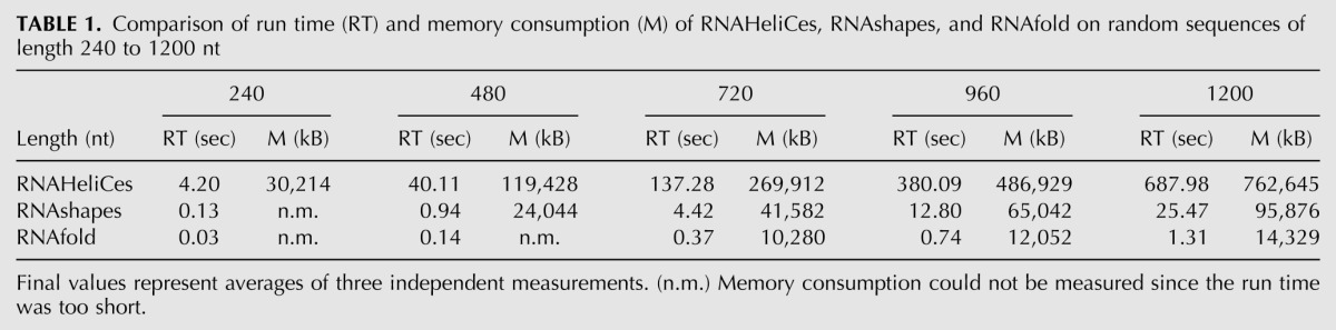
We measured run time and memory consumption for RNAHeliCes, RNAshapes (Steffen et al. 2006), and RNAfold (Hofacker et al. 1994). The results are summarized in Table 1. Overall, RNAfold performs best, followed by RNAshapes and RNAHeliCes. Setting the results of RNAfold to 1 gives a run time relationship of 1:20:600 and a memory consumption relationship of 1:8:50. Reasons for the comparably long run time of RNAHeliCes are the use of a more complex grammar, resembling RNAsubopt, and the use of automatically generated, not manually optimized, code. Similar considerations apply for the memory consumption.

TABLE 1.

Comparison of run time (RT) and memory consumption (M) of RNAHeliCes, RNAshapes, and RNAfold on random sequences of length 240 to 1200 nt

Energy barrier estimation

Important features of the folding space are pathways connecting alternative structures. For these pathways, commonly the most interesting features are the saddle structure and its energy, from which the energy barrier can be calculated. Computation of these folding pathways within our program HiPath follows the idea of a guided path. Guide points are provided by hishapes, and, in order to achieve a reasonably fast method, the paths between guide points are computed heuristically. For this, we chose breadth first search, which has already been used for pathway approximation in Flamm et al. (2001). Unlike Morgan-Higgs, BFS keeps the l best intermediate results at each iteration step, which significantly increases prediction accuracy. We provide two methods—one, called HiPath-full, for predicting energy barriers for all pairs of hishapes, and the other, named HiPath-pair, for predicting the energy barrier for a given pair of structures/hishapes.

Full method for barrier estimation

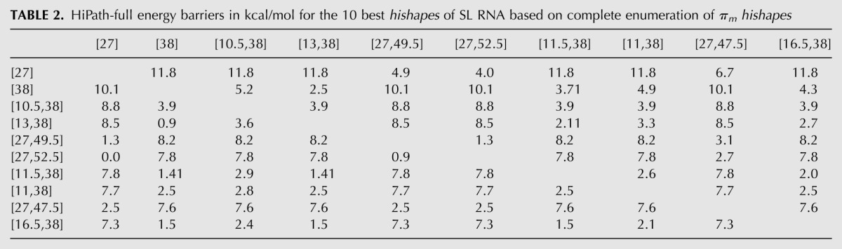
For a complete folding space analysis, we start with computing all hishapes of interest (e.g., all or the k = 100 best). For all possible pairs, we compute a near-optimal pathway using BFS (e.g., l = 10) on the hishreps and store its saddle structure and energy in a matrix. For vicinal hishapes, i.e., hishapes with similar hishreps, the BFS results can be expected to be good, but for distant hishapes, they can very likely be improved. We do this by applying Dijkstra's algorithm (Dijkstra 1959) to compute optimal paths based on the initial results. The improvement is a result of combining short, more accurate paths into long ones. We applied the HiPath-full procedure to all (N = 3535) π_m hishapes of the SL RNA (56 nt). Results for the 10 best hishapes are summarized in Table 2. For example, the pathway from [27] to [38] has an energy barrier of 11.8 kcal/mol. Compared to the exact value from Barriers—11.1 kcal/mol, our method is 0.7 kcal/mol or ∼6% wrong. Another interesting feature can be figured out when looking at the rows for hishapes [27] and [38]. Whenever hishape [27] is compared to a hishape containing helix 38, the energy barrier is equally high (11.8 kcal/mol), while it is lower for those hishapes containing helix 27 (at most, 6.7 kcal/mol). For hishape [38], it is vice versa. Thus, helices 27 and 38 are kinetically incompatible, which nicely reflects the bistable character of this RNA.

TABLE 2.

HiPath-full energy barriers in kcal/mol for the 10 best hishapes of SL RNA based on complete enumeration of π_m hishapes

Pairwise barrier approximation

In our results, we empirically found that the number of hishapes grows exponentially with sequence length. Thus, in general the full procedure is computationally very expensive. So, how can we improve? Consider the case that we are only interested in computing the energy barrier for a certain start and target structure. How can we reasonably restrict the number of hishapes without losing analysis depth? Here, we make use of related hishapes as defined by Equation 5. Related hishapes are those hishapes where each hairpin loop helix index is present in the hishape of start and/or the target structure. They can be computed using a modified grammar in which a syntactic filter is applied to the productions for hairpin loops. This filter checks to see if the hairpin loop is an element of the union of hairpin loop helix indices of the start and target structure. With this approach, we compute rigorously all related hishapes in a very lean and, thus, fast way. For the set of related hishapes, we apply the same procedure as described above, with the difference that we use Dijkstra's algorithm to compute the optimal path for the user-defined start and target structure/hishape only.

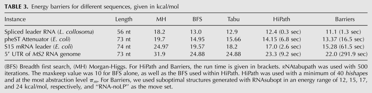
In order to assess the accuracy of our approximation, we used data set “short” (see Materials and Methods) to compare our algorithm to four other methods, namely Barriers, Morgan-Higgs (MH), BFS with 10 best candidates, and RNAtabupath (Dotu et al. 2010). The results in Table 3 show that the hishape-based pathway approximation performs best compared to the other heuristics and achieves reasonable accuracy when compared with the exact results from Barriers. The error ranges from 0.78 to 1.72 kcal/mol and is, in all cases, ≤12%. HiPath was, in all cases, 4–30 times faster than Barriers.

TABLE 3.

Energy barriers for different sequences, given in kcal/mol

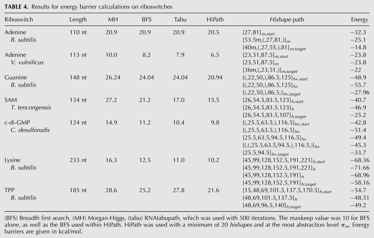
In order to get an impression of the source of the inaccuracy of our method, we compared the saddle structures and hishapes predicted by our method with the “native” ones computed by Barriers (data not shown). Interestingly, in all cases, the native saddle structure comprises helices (hairpin loops) that were not present in the start or target structure. Thus, the hishape of the native saddle does not belong to the set of related hishapes. Furthermore, the BFS step of our procedure does not compensate for this error, at least for the cases shown. Overall, it seems that the energetically most favorable pathway is more complex than expected. We performed a second benchmark using the data set “riboswitches” (see Materials and Methods). The results in Table 4 show that our algorithm is able to compute better folding pathways in all cases. We can improve the estimated energy barrier by 0.4–3.6 kcal/mol or by ∼1.6 kcal/mol on average.

TABLE 4.

Results for energy barrier calculations on riboswitches

Performance

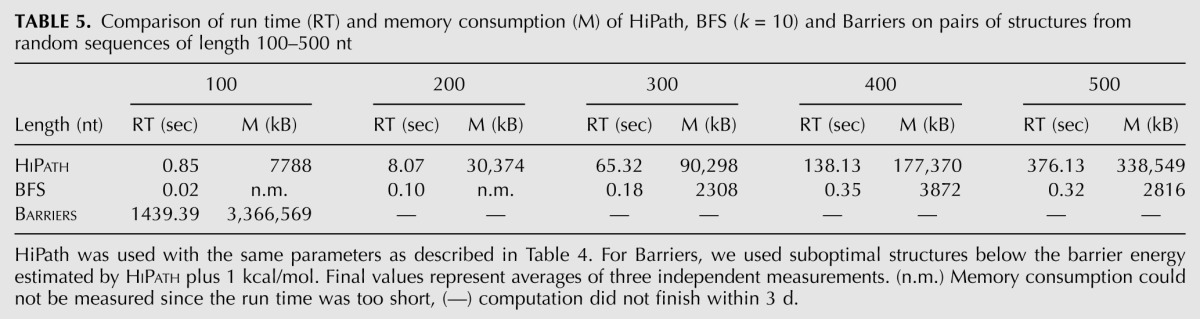
The efficiency of our algorithm strongly depends on related hishape calculation that is carried out by RNAHeliCes. On a typical sequence, e.g., the lysine riboswitch of lysC from Bacillus subtilis (233 nt), the run time remains <50 sec. In order to get a general picture, we measured run time and memory consumption of HiPath, BFS, and Barriers. The results are given in Table 5. Barriers produced results within a reasonable time only for sequences up to 100 nt in length. BFS is the fastest and least expensive method. HiPath performs quite well and computes the energy barrier for two structures of length 500 nt in ∼6 min, consuming ∼340 MB of memory.

TABLE 5.

Comparison of run time (RT) and memory consumption (M) of HiPath, BFS (k = 10) and Barriers on pairs of structures from random sequences of length 100–500 nt

Abstract structure comparison

Another feature of interest when analyzing the folding space of an RNA is structural diversity. For hishapes, i.e., hishreps, we can, of course, use existing methods for structure comparison, and they would benefit from the reduced number of entities that need to be compared. But why not design a comparative approach solely based on hishapes? They are inherently tree-like, and the positional information provides reasonable resolution for comparison.

We introduce the hishape-based tree edit distance (HiTed), which is an extension of the tree edit distance (Shapiro 1988). Our method extends the tree edit distance for abstract trees of RNA secondary structures (Shapiro and Zhang 1990). This representation abstracts from the size of structural elements and is, thus, closely related to the idea of abstract shapes. In Shapiro and Zhang (1990), the edit operations—relabeling, delete, and insert—and a corresponding cost function for edit operations on abstract trees are defined.

HiTed is based on this scoring scheme for loop/helix editing and extends it by the positional distance of helices. The latter is the absolute difference of the helix indices, e.g., d(35i, 45i) = |35 – 45| = 10. The two distance measures are combined using a weighting factor λ as shown in Definition 6 (Materials and Methods). The initial intention in the design of HiTed was to have a distance measure for alternative hishapes of the same sequence. Nevertheless, we think that HiTed is also suitable for comparing structures/hishapes of different sequences. In order to assess this and to analyze the influence of the weighting factor λ, we provide two benchmarks. First, we compare the results for different λ-values, and, second, we compare HiTed with other structure comparison methods, namely RNAdistance (Hofacker et al. 1994) and RNAforester (Höchsmann et al. 2003). We do this using the Brasero data set and protocol (see Materials and Methods). We take the area under the curve (AUC) values of the ROC plots to visualize the results. Figure 3 shows how the AUC changes with 0 ≤ λ ≤ 32. Overall, there seems to be no general optimal λ-value, but a range of 0 to 5 seems to be reasonable to achieve reliable results. For SRP and sRNA, the additional positional distance introduced by HiTed improves prediction accuracy, and we achieve the best results with values of 17 and 2, respectively. Conversely, for the miRNA and tRNA data sets, the performance decreases with increasing λ, and the optimum is λ = 0 for these data sets. One reason for this might be that the helices occur at quite diverse positions within the sequences, thus the penalization of the positional difference decreases performance.

FIGURE 3.

Benchmarking the weight factor λ. For each data set, namely SRP, sRNA, miRNA, and tRNA, the area under the curve (AUC) of the ROC curve with regard to the background set, either “viral” or “encode,” is plotted for varying λ. Note that the SRP data set is provided containing only “viral” background data.

We compare HiTed with RNAdistance and RNAforester. For HiTed, we chose two different values for λ. λ = 5 resembles a consensus value based on the previous results, and λ = 0 switches off the positional distance contribution. The latter is similar to using RNAdistance in the coarse-grained tree editing mode, the distance measure introduced by Shapiro and Zhang (1990). We refer to this as RNAdistance_SZ, compared to RNAdistance using default parameters, i.e., tree editing on full structure representation. Finally, RNAforester was used once with default parameters and once without scoring sequence homology (RNAforester_NOSEQ). Results are shown in Figure 4. Interestingly, our abstract and fast comparative analysis of RNA achieves the second best accuracy for one data set (SRP) and comparable results for the other data sets. The SRP data set seems to be tricky, since, for all three tools, the variant that takes more information into account performs better. The opposite situation appears for the miRNA data set. For this data set, only RNAforester shows good performance and the other methods perform rather poorly. Here, one reason may lie in the fact that a single hairpin structure, being the structure of miRNA precursors, is quite likely to occur in random sequences, thus increasing the false positive rate. Looking into the noise part of the miRNA data set shows that this is actually the case. Additionally, the diversity of the T2 set is large as it contains sequences with up to 188 nt, while the sequences in R and F2 are at most 87 and 88 nt long, respectively. Albeit HiTed with λ = 0 and RNAdistance_SZ seem conceptually similar, their performance differs reasonably. The coarse-grained tree representation differs from the hishape tree in that it also models stacking regions and the external loop, which presumably is the reason for these differences.

FIGURE 4.

ROC plots comparing HiTed, RNAdistance, and RNAforester on data sets SRP (A), sRNA (B), miRNA (C), and tRNA (D). The noise data used in all four cases are random genome segments from viral genomes. RNAdistance was used with default parameters (tree edit distance on full structure representation) and with coarse-grained tree edit distance (Shapiro and Zhang 1990) RNAdistance_SZ. RNAforester was used with default parameters and without scoring sequence similarity (RNAforester_noseq). HiTed was used with the indicated λ-values.

Performance

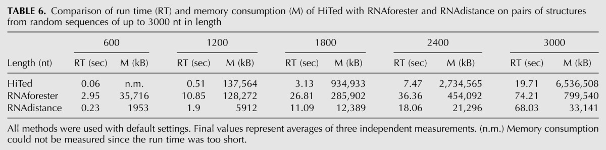
We compared the run time and memory consumption of HiTed (λ = 5) with RNAdistance and RNAforester. The results in Table 6 show that HiTed is the fastest but also the most memory-consuming method. The latter fact is an implementation issue and can thus be resolved by optimizing the code.

TABLE 6.

Comparison of run time (RT) and memory consumption (M) of HiTed with RNAforester and RNAdistance on pairs of structures from random sequences of up to 3000 nt in length

DISCUSSION

In the present paper, we introduce the concept of hishapes, which is closely related to the idea of abstract shapes. Briefly, we provide new mapping functions and preserve all functionality of shape analysis. Among these are search space reduction by (hi)shape filtering and probabilistic analysis based on (hi)shape classes. Compared to abstract shapes, the major advantage of the new abstraction is its position-specificity, which provides a better resolution, especially for short RNAs. The cost for this is a slightly increased search space, which is still much smaller than the structure space. Nevertheless, the abstraction keeps significant features of the structure space. Although the mathematical proof is not yet provided, based on our preliminary empirical analyses, we are convinced that hishapes comprise all, or at least a significant subset, depending on the abstraction level, of local minima of the folding space. Important features when analyzing the folding space of RNA are the energy barriers separating local minima. Their exact computation is expensive, and thus, several heuristic methods have been developed to allow for the analysis of long sequences and also to greater depth. HiPath, our hishape-guided energy barrier calculation, belongs to these methods and outperforms all heuristic methods compared in this manuscript. Comparing HiPath predictions for short sequences with exact values computed with Barriers shows that the inaccuracy is, in general, ∼10%. Taking into account the inaccuracies of the thermodynamic parameters and that we neglect kinetic effects, the pathways and hence, the energy barriers predicted by RNAHeliCes provide reasonable alternatives.

The kinetics of RNA folding will be a major aspect in our future work on RNAHeliCes. In all abstraction levels we present, hairpin loops and their associated helices play a major role. For a helix closed by a hairpin loop, the helix index corresponds to the center of the closing base pair of the hairpin loop. The nucleation of the helix, formation of a hairpin loop, is the rate-limiting step in helix formation where, according to the master equation, the rate is dependent on the gain/loss in free energy. Thus, the thermodynamically most favorable hairpin loop is also the most likely to be formed first. Such a helix-based approach for predicting folding kinetics has been presented by Zhao et al. (2010). Their move set comprises helix addition, helix deletion, arm-by-arm exchange, and two-arm by two-arm exchange, which all fit perfectly into the hishape model. Together with the method for fast energy barrier computation, hishapes provide a promising candidate for kinetic studies.

So far, we have discussed the thermodynamic and perhaps kinetic capabilities of RNAHeliCes. Commonly, also structural characteristics of the folding space are of interest. For this purpose, we introduced the hishape-based tree edit distance (HiTed). The performance of HiTed is comparable to those of other commonly used methods. This is somewhat surprising, taking into account the abstract tree representation on which it is based and the somewhat arbitrary scoring scheme it uses. Probably, the abstraction helps, at least in some cases, to circumvent pitfalls that the algorithms working on the full tree representation face. The scoring scheme likely needs some refinements, which may also be accompanied by changing the representation of helix indices. The currently used absolute position will disturb results when common structures are shifted within related sequences by insertions or elongated 5′ UTRs. Here, for example, relative positional values might be better suited. Additionally, choosing a reasonable value for parameter λ is important in achieving optimal results. A good choice depends on various factors, such as sequence similarity, expected structural diversity, and the aim of the analysis. Therefore, it is difficult to provide a rule of thumb, but comparing the results for different values of λ should help in this process.

A combination of the methods presented might include the idea of predicting conformational switching followed by paRNAss. Here, a conformational switch is characterized by the existence of two local minima that are structurally dissimilar and separated by a reasonable energy barrier. Furthermore, RNAHeliCes and HiTed might be used for the identification of common structures of two or more RNAs. This would provide an alternative to the prediction of consensus shapes (Reeder and Giegerich 2005).

Altogether, we believe that hishape-based abstraction provides a valuable tool for various applications in RNA secondary structure analysis. Improvements may be achieved for run time and memory usage by manual optimizations of the code generated by the GAP compiler. On the conceptual side, modified abstractions based on other helix features, e.g., outermost base pair, may be useful and extend the range of applications for our method.

MATERIALS AND METHODS

Defining helix index shapes

In the following, we provide formal definitions for the new abstraction based on helix indices. We consider unknotted secondary structures as defined, for example, in Hofacker et al. (1994).

Definition 1 (helix and helix index)

A helix is a series of stacking base pairs starting with the closing base pair of a hairpin, bulge, internal, or multiple loop (hl, bl, il, or ml, respectively). Thus, a helix can be denoted by h_L (i, j) where i and j are the bases of the innermost base pair and L is the loop type (L ∈ {hl, bl, il, ml}). The helix index of a helix h_L (i, j) is its central position, thus

Definition 2 (hishape, hishrep, and hishape space)

Any RNA secondary structure can be transformed into a list of helices H. Using mapping functions π_h, π_h+, π_m, or π_a, we can map H to a list of helix indices which we term hishape (helix index shape).

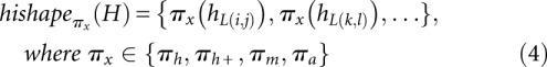π_h and π_h+ retain only hairpin loop helices, while π_m and π_a additionally retain multiloop and all helices, respectively. Except for π_h, all abstractions preserve the nesting pattern of helices by embracing helices within multiloops by a pair of brackets. Note that the mapping defined in Equation 4 does not ensure the correct nesting of helices by itself. This has to be achieved via the correct evaluation order within the algorithm, which is discussed in Materials and Methods. For π_m and π_a, hishapes may be ambiguous since multiloop and symmetric internal loop helices can have helix indices equal to their enclosed helices. Therefore, the letter “m” is attached to the end of helix indices derived from h_ml(i, j) in π_m as well as in π_a, while the letter “b” denotes helix indices derived from h_bl(i, j), and the letter “i” denotes helix indices derived from h_il(i, j) in π_a.

Definition 3 (Related hishapes)

Given two hishapes H₁ and H₂ in an arbitrary abstraction type, and let ϕ be a function extracting hairpin loop helix indices, related hishapes H_r are those satisfying

Implementation

In order to circumvent implementation-specific problems, e.g., index errors, and to take advantage of already existing code, we implemented the algorithms using Bellman's GAP (Giegerich and Sauthoff 2011; Sauthoff et al. 2011). Here, a DP algorithm is split into a grammar and several algebras. The grammar ensures the correct nesting and juxtaposition of structural elements and, thus, describes the candidates of the search space, while the algebras evaluate these candidates. In the case of RNA structure analysis, algebras for energy minimization, partition function (McCaskill 1990) calculation, and pretty printing of the structure in dot-bracket-format and others exist. Algebras can be combined using product operations, which allow complex analyses to be built in a rather simple way. We make use of two different grammars. For probabilistic analysis, we use the grammar which handles dangling bases in an unambiguous fashion (Voß et al. 2006), while hishape prediction is based on the “microstate” grammar described in Janssen et al. (2011). The latter resembles RNAsubopt with the “-d2” option for dangle energy correction. Note that this grammar is ambiguous and can thus not be used for probabilistic analysis. In RNAHeliCes, for each candidate defined by the grammar, we are interested in computing the hishape, the free energy, the dot-bracket-representation, and, for probabilistic analysis, the partition function contribution of this hishape. We can reuse existing algebras for computation of free energy, partition function, and dot-bracket-representation. The algebra for computation of hishapes was developed by us and implemented as described in the following. Thermodynamic parameters (Xia et al. 1998; Mathews et al. 1999, 2004; Schroeder and Turner 2000) used within Bellman's GAP are taken from the Vienna RNA package (Hofacker et al. 1994).

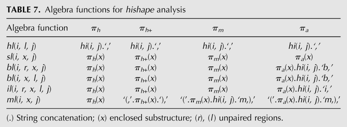
Algebra hishape has four different abstraction levels according to the four mapping functions π_h, π_h+, π_m, and π_a. Table 7 shows how this is reflected within the algebra functions for the different loop/helix types. The choice function h unifies candidates with equal hishape resulting in nonredundant answer lists. Our goal is to compute hishapes together with their free energy, partition function contribution, and the hishrep in dot-bracket notation. Reusing the algebras mfe for free energy calculation, p_func for partition function values, and pretty for the dot-bracket-representation, in GAP we can achieve this with the algebra product: hishape ⊗ (mfe × p_func) * pretty, where ⊗ is the interleaved, × the Cartesian, and * the lexicographic product operation. Details about these product types can be found in Giegerich and Sauthoff (2011) and Sauthoff et al. (2011).

TABLE 7.

Algebra functions for hishape analysis

Because of the exponential growth of hishape classes (see Results), k ≈ αⁿ, where α depends on the mapping function π, and the time complexity would be O(αⁿ). However, an implementation returning only the k-best (for example, k = 100) hishape classes reduces the overall complexity to O(k²n³). It is important to note that k-best computation cannot be used to compute correct hishape probabilities. The reason for this is that the probability calculation is based on a hishape-wise summation of Boltzmann-weighted energies. Whenever a hishape is not among the k best for the current subword, its Boltzmann-weighted energy will not contribute to the final result for this hishape, thus leading to inaccurate results. This error decreases with larger k, but to what extent has to be thoroughly investigated.

Approximating folding pathways

Full pathway analysis

The method for computing all pairwise energy barriers for a set of hishapes of an RNA sequence is as follows: First, compute all pairwise paths using BFS, and store saddle structure in matrix M_BFS. Second, use Dijkstra's algorithm to find the shortest path in M_BFS for all pairs of hishapes. The procedure is given in algorithm 1.

ALGORITHM 1. HiPath-full.

L ← List of (hishapes,hishreps)

N ← Length (L)

for i = 1 → N do

for j = 1 → N do

M_BFS (L[i], L[j]) ← BFS(L[i],L[j]) ▷breadth first search

end for

end for

for i = 1 → N do

M (L[i], _) ← ShortestPath(L[i], M_BFS) ▷Dijkstra's algorithm; single source, all targets

end for

return M

We use findpath.h from the Vienna RNA package v1.7.2 for BFS computation. This algorithm computes the full matrix, and as a result, this matrix holds two saddle structures for each pair of hishapes/structures. In many cases, they will be the same, but especially for longer sequences, they may be different, corresponding to the fact that different pathways have been predicted for the forward and backward reaction. When computing energy barriers for individual pairs we take the saddle with lower free energy.

Definition 4 (HiPath energy barrier)

For a given start structure S and target structure T and given that the function HiPath(i, j) computes the saddle structure of a pathway from structure i to structure j and ΔG(X) is the free energy of structure X

Pairwise pathway approximation

For the computation of a single pathway between a given start and target structure, we restrict the search space to related hishapes as defined by Equation 5. Additionally, only the shortest path from the start to the target structure is computed. An outline is shown in algorithm 2.

ALGORITHM 2. HiPath-pair.

S ← start structure, T ← target structure

H_S ← Hishape_h(S), H_T ← Hishape_h(T) ▷ Hishape_h returns hairpin loop helix indices only

H_U ← H_S ∪ H_T

L ← RNAHeliCes -m H_U ▷ Compute related hishapes

N ← Length (L)

for i = 1 → N do

for j = 1 → N do

M_BFS (L[i], L[j]) ← BFS(L[i],L[j]) ▷ breadth first search

end for

end for

return ShortestPath(H_S, H_T, M_BFS) ▷ Dijkstra's algorithm; single source, single target

The number of (related) hishapes has a large impact on the speed of the procedure, and thus we provide means to reasonably restrict it. The calculation of (related) hishapes always starts at the most abstract level. If, in this level the number of hishapes does not reach a user defined threshold n, the next less-abstract level is used. This is done either until the threshold n or a user-defined, lowest abstraction level t is reached.

Abstract structure comparison

Any RNA secondary structure can be represented as a node-labeled tree (Zuker and Sankoff 1984; Shapiro 1988; Shapiro and Zhang 1990), and this representation was shown to be especially useful for comparative purposes, such as distance computation and alignment. Hishapes are also inherently tree-like and can thus be represented as trees, too. An example is shown in Figure 5, and the definition is as follows.

FIGURE 5.

Hishape tree representation of the π_a hishape [36m,(,17,35.5i,35.5b,36,56,),] of the example secondary structure in Fig. 1A.

Definition 5 (hishape tree)

A hishape tree T consists of a set of helix nodes N that are connected by edges. Each N is a tuple (c,t) where c is the helix index and t the helix type, t ∈ (h, m, i, b). If the hishape does not provide the helix index for a certain node, as is the case for multiloop helices in abstraction π_h+, c is set to −1. An edge represents a parent-child relationship according to the nesting of helices. Any T has a root node (0, e) that corresponds to the external loop. The hishape tree of the empty structure consists of only the root node.

For the comparison of two hishape trees, we follow the idea of tree editing (Zhang and Shasha 1989), which was already applied to abstract trees of RNA secondary structures, where only the loops/helices are represented (Shapiro and Zhang 1990). Here, edit operations act on complete loops/helices which perfectly suits the idea of hishapes. In order to make use of the additional positional information provided by hishapes, we extend the scoring and define the hishape-based tree edit distance (HiTed).

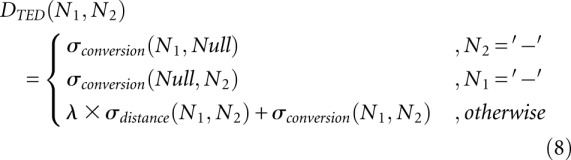
Definition 6 (hishape-based tree edit distance [HiTed])

The three edit operations—relabeling, delete, and insert—can be represented as pairs (a,b), (a,−), (−,b), respectively. Given two hishape trees T₁ and T₂ and a sequence S = s₁, …, s_k of edit operations

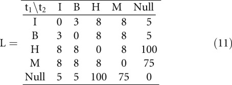The first alternative in Equation 9 considers the case of a multiloop helix, for which no helix index is given in abstraction type π_h+. Values in Equation 11 are taken from Shapiro and Zhang (1990).

In order to find the set of edit operations that minimizes HiTed, we make use of dynamic programming as has been presented by Zhang and Shasha (1989). The implementation makes use of functions from RNA StrAT (Guignon et al. 2005).

Benchmarking data sets and procedures

Data set “short”

Data set “short” is based on the four shortest sequences from the paRNAss evaluation (Voß et al. 2004), namely spliced leader RNA (L. collosoma), pheST Attenuator (Escherichia coli), S15 mRNA leader (E. coli), and the 5′ UTR of MS2 RNA genome. We selected these sequences in order to facilitate a reasonable run time of Barriers, which grows exponential with sequence length and is limited to ∼150 nt. For each sequence, the minimum free energy structure was taken as structure A, and a target structure B was determined using the following procedure: predict hishapes using π_h, scan the energy sorted hishape list for a hishape for which each helix index differs by more than 5 from each helix index of structure A.

Data set “riboswitches”

This data set is taken from Li and Zhang (2011) and provides a compilation of seven riboswitch sequences, namely the adenine riboswitch of ydhL gene from B. subtilis (Mandal and Breaker 2004), the adenine riboswitch of add gene from Vibrio vulnificus (Lemay et al. 2011), the guanine riboswitch of xpt-pbuX operon from B. subtilis (Mandal et al. 2003), the S-adenosylmethionine riboswitch of metE from Thermoanaerobacter tencongensis (Epshtein et al. 2003), the c-di-GMP riboswitch of the tfoX from Candidatus desulforudis (Smith et al. 2009), the lysine riboswitch of the lysC from B. subtilis (Blouin et al. 2011), and the thiamine pyrophosphate riboswitch of thiamin from B. subtilis (Mironov et al. 2002; Rentmeister et al. 2007). Most important about this data set is that it provides the native “on” and “off” conformations of the riboswitches. This allows benchmarking the methods in a realistic scenario.

Data set and benchmark procedure for structure comparison

For the structure-comparative benchmarks, we took four different data sets from the Brasero (Allali et al. 2012) collection, namely SRP, sRNA, miRNA, and tRNA. Each data set consists of three parts: The first one is a small number of RNAs together with their known structures R of the given RNA family F; the second is a set of RNA secondary structures T2 folded from a set of RNA sequences that belong to F using mfold (Zuker and Stiegler 1981) or RNAshapes; and the third, called noise, is a set of RNA secondary structures F2 folded from a set of RNA sequences that are either random segments from viral genomes or from encode sequences.

In Brasero, benchmarking is performed by comparing each structure of T2 and F2 with each structure of R using the given pairwise comparison algorithm. Depending on the score, structures of T2 and F2 can now be classified as true positives, false negatives, false positives, and true negatives. Iterating from the minimum to the maximum score, computing for each the true and false positive rate and plotting these values against each other results in a ROC plot. All this is done by the benchmarking tools provided by Brasero, which also compute the area under the curve of the ROC plot.

Measuring run time and memory consumption

For memory usage measurements, we monitored the VmHWM (“high water mark”) value in the /proc file system. The run time is the CPU time (sum of user and system time) as measured using GNU time. All measurements were carried out on an 8x AMD Opteron 8378 machine with 128 GB RAM under openSUSE 11.2 (x86_64).

REFERENCES

- Allali J, Saule C, Chauve C, d'Aubenton-Carafa Y, Denise A, Drevet C, Ferraro P, Gautheret D, Herrbach C, Leclerc F, et al. 2012. BRASERO: A resource for benchmarking RNA secondary structure comparison algorithms. Adv Bioinforma 2012: 1–5 [DOI] [PMC free article] [PubMed] [Google Scholar]
- Blouin S, Chinnappan R, Lafontaine D 2011. Folding of the lysine riboswitch: Importance of peripheral elements for transcriptional regulation. Nucleic Acids Res 39: 3373–3387 [DOI] [PMC free article] [PubMed] [Google Scholar]
- Bogomolov S, Mann M, Voß B, Podelski A, Backofen R 2010. Shape-based barrier estimation for RNAs. In Proceedings of German conference on bioinformatics (ed. D Schomburg, A Grote), Lecture notes in informatics, Vol. 173, pp. 41–50. Technische Universität Carolo Wilhelmina zu Braunschweig, Braunschweig, Germany [Google Scholar]
- Darty K, Denise A, Ponty Y 2009. VARNA: Interactive drawing and editing of the RNA secondary structure. Bioinformatics 25: 1974–1975 [DOI] [PMC free article] [PubMed] [Google Scholar]
- Dijkstra E 1959. A note on two problems in connexion with graphs. Numer Math 1: 269–271 [Google Scholar]
- Dotu I, Lorenz W, Van Hentenryck P, Clote P 2010. Computing folding pathways between RNA secondary structures. Nucleic Acids Res 38: 1711–1722 [DOI] [PMC free article] [PubMed] [Google Scholar]
- Epshtein V, Mironov A, Nudler E 2003. The riboswitch-mediated control of sulfur metabolism in bacteria. Proc Natl Acad Sci 100: 5052–5056 [DOI] [PMC free article] [PubMed] [Google Scholar]
- Flamm C, Fontana W, Hofacker I, Schuster P 2000. RNA folding at elementary step resolution. RNA 6: 325–338 [DOI] [PMC free article] [PubMed] [Google Scholar]
- Flamm C, Hofacker I, Maurer-Stroh S, Stadler P, Zehl M 2001. Design of multistable RNA molecules. RNA 7: 254–265 [DOI] [PMC free article] [PubMed] [Google Scholar]
- Flamm C, Hofacker I, Stadler P, Wolfinger M 2002. Barrier trees of degenerate landscapes. Z Phys Chem 216: 155–173 [Google Scholar]
- Giegerich R, Sauthoff G 2011. Yield grammar analysis in the Bellman's GAP compiler. In Proceedings of the eleventh workshop on language descriptions, tools and applications. doi: 10.1145/1988783.1988790. Association for Computing Machinery, New York [Google Scholar]
- Giegerich R, Voß B, Rehmsmeier M 2004. Abstract shapes of RNA. Nucleic Acids Res 32: 4843–4851 [DOI] [PMC free article] [PubMed] [Google Scholar]
- Guignon V, Chauve C, Hamel S 2005. An edit distance between RNA stem-loops. In Proceedings of the twelfth international conference on string processing and information retrieval (ed. M Consens, G Navarro), Lecture notes in computer science, Vol. 3772, pp. 335–347. Springer, Berlin/Heidelberg, Germany [Google Scholar]
- Höchsmann M, Töller T, Giegerich R, Kurtz S 2003. Local similarity in RNA secondary structures. In Proceedings of the IEEE bioinformatics conference, pp. 159–168. IEEE, New York [PubMed] [Google Scholar]
- Hofacker IL, Fontana W, Stadler PF, Bonhoeffer SL, Tacker M, Schuster P 1994. Fast folding and comparison of RNA secondary structures. Monatsh Chem 125: 167–188 [Google Scholar]
- Janssen S, Schudoma C, Steger G, Giegerich R 2011. Lost in folding space? Comparing four variants of the thermodynamic model for RNA secondary structure prediction. BMC Bioinformatics 12: 429 doi: 10.1186/1471-2105-12-429 [DOI] [PMC free article] [PubMed] [Google Scholar]
- LeCuyer K, Crothers D 1993. The Leptomonas collosoma spliced leader RNA can switch between two alternate structural forms. Biochemistry 32: 5301–5311 [DOI] [PubMed] [Google Scholar]
- Lemay J, Desnoyers G, Blouin S, Heppell B, Bastet L, St-Pierre P, Massé E, Lafontaine D 2011. Comparative study between transcriptionally- and translationally-acting adenine riboswitches reveals key differences in riboswitch regulatory mechanisms. PLoS Genet 7: e1001278 doi: 10.1371/journal.pgen.1001278 [DOI] [PMC free article] [PubMed] [Google Scholar]
- Li Y, Zhang S 2011. Finding stable local optimal RNA secondary structures. Bioinformatics 27: 2994–3001 [DOI] [PubMed] [Google Scholar]
- Lorenz W, Ponty Y, Clote P 2008. Asymptotics of RNA shapes. J Comput Biol 15: 31–63 [DOI] [PubMed] [Google Scholar]
- Mandal M, Breaker R 2004. Adenine riboswitches and gene activation by disruption of a transcription terminator. Nat Struct Mol Biol 11: 29–35 [DOI] [PubMed] [Google Scholar]
- Mandal M, Boese B, Barrick J, Winkler W, Breaker R 2003. Riboswitches control fundamental biochemical pathways in Bacillus subtilis and other bacteria. Cell 113: 577–586 [DOI] [PubMed] [Google Scholar]
- Mathews DH, Sabina J, Zuker M, Turner DH 1999. Expanded sequence dependence of thermodynamic parameters improves prediction of RNA secondary structure. J Mol Biol 288: 911–940 [DOI] [PubMed] [Google Scholar]
- Mathews D, Disney M, Childs J, Schroeder S, Zuker M, Turner D 2004. Incorporating chemical modification constraints into a dynamic programming algorithm for prediction of RNA secondary structure. Proc Natl Acad Sci 101: 7287–7292 [DOI] [PMC free article] [PubMed] [Google Scholar]
- McCaskill JS 1990. The equilibrium partition function and base pair binding probabilities for RNA secondary structure. Biopolymers 29: 1105–1119 [DOI] [PubMed] [Google Scholar]
- Mironov A, Gusarov I, Rafikov R, Lopez L, Shatalin K, Kreneva R, Perumov D, Nudler E 2002. Sensing small molecules by nascent RNA: A mechanism to control transcription in bacteria. Cell 111: 747–756 [DOI] [PubMed] [Google Scholar]
- Morgan S, Higgs P 1998. Barrier heights between ground states in a model of RNA secondary structure. J Phys Math Gen 31: 3153 doi: 10.1088/0305-4470/31/14/005 [Google Scholar]
- Nebel M, Scheid A 2009. On quantitative effects of RNA shape abstraction. Theory Biosci 128: 211–225 [DOI] [PubMed] [Google Scholar]
- Reeder J, Giegerich R 2005. Consensus shapes: An alternative to the Sankoff algorithm for RNA consensus structure prediction. Bioinformatics 21: 3516–3523 [DOI] [PubMed] [Google Scholar]
- Rentmeister A, Mayer G, Kuhn N, Famulok M 2007. Conformational changes in the expression domain of the Escherichia coli thiM riboswitch. Nucleic Acids Res 35: 3713–3722 [DOI] [PMC free article] [PubMed] [Google Scholar]
- Sauthoff G, Janssen S, Giegerich R 2011. Bellman's GAP—a declarative language for dynamic programming. In Proceedings of 13th international ACM SIGPLAN symposium on principles and practice of declarative programming, pp. 29–40. Association for Computing Machinery, New York [Google Scholar]
- Schroeder SJ, Turner DH 2000. Factors affecting the thermodynamic stability of small asymmetric internal loops in RNA. Biochemistry 39: 9257–9274 [DOI] [PubMed] [Google Scholar]
- Shapiro B 1988. An algorithm for comparing multiple RNA secondary structures. Comput Appl Biosci: CABIOS 4: 387–393 [DOI] [PubMed] [Google Scholar]
- Shapiro B, Zhang K 1990. Comparing multiple RNA secondary structures using tree comparisons. Comput Appl Biosci 6: 309–318 [DOI] [PubMed] [Google Scholar]
- Smith K, Lipchock S, Ames T, Wang J, Breaker R, Strobel S 2009. Structural basis of ligand binding by a c-di-GMP riboswitch. Nat Struct Mol Biol 16: 1218–1223 [DOI] [PMC free article] [PubMed] [Google Scholar]
- Steffen P, Voss B, Rehmsmeier M, Reeder J, Giegerich R 2006. RNAshapes: An integrated RNA analysis package based on abstract shapes. Bioinformatics 22: 500–503 [DOI] [PubMed] [Google Scholar]
- Voß B, Meyer C, Giegerich R 2004. Evaluating the predictability of conformational switching in RNA. Bioinformatics 20: 1573–1582 [DOI] [PubMed] [Google Scholar]
- Voß B, Giegerich R, Rehmsmeier M 2006. Complete probabilistic analysis of RNA shapes. BMC Biol 5: 4 doi: 10.1186/1741-7007-4-5 [DOI] [PMC free article] [PubMed] [Google Scholar]
- Wuchty S, Fontana W, Hofacker I, Schuster P 1999. Complete suboptimal folding of RNA and the stability of secondary structures. Biopolymers 49: 145–165 [DOI] [PubMed] [Google Scholar]
- Xia T, SantaLucia J, Burkard ME, Kierzek R, Schroeder SJ, Jiao X, Cox C, Turner DH 1998. Thermodynamic parameters for an expanded nearest-neighbor model for formation of RNA duplexes with Watson–Crick base pairs. Biochemistry 37: 14719–14735 [DOI] [PubMed] [Google Scholar]
- Zhang K, Shasha D 1989. Simple fast algorithms for the editing distance between trees and related problems. SIAM J Comput 18: 1245–1262 [Google Scholar]
- Zhao P, Zhang W, Chen S 2010. Predicting secondary structural folding kinetics for nucleic acids. Biophys J 98: 1617–1625 [DOI] [PMC free article] [PubMed] [Google Scholar]
- Zuker M, Sankoff D 1984. RNA secondary structures and their prediction. Bull Math Biol 46: 591–621 [Google Scholar]
- Zuker M, Stiegler P 1981. Optimal computer folding of large RNA sequences using thermodynamics and auxiliary information. Nucleic Acids Res 9: 133–148 [DOI] [PMC free article] [PubMed] [Google Scholar]