

Abstract
Aim
The aim of this paper was to demonstrate the usage of an automated computer-based IMT measurement system called - CALEX 3.0 (a class of patented AtheroEdge™ software) on a low contrast and low resolution image database acquired during an epidemiological study from India. The image contrast was very low with pixel density of 12.7 pixels/mm. Further, to demonstrate the accuracy and reproducibility of the AtheroEdge™ software system we compared it with the manual tracings of a vascular surgeon – considered as a gold standard.
Methods
We automatically measured the IMT value of 885 common carotid arteries in longitudinal B-Mode images. CALEX 3.0 consisted of a stage for the automatic recognition of the carotid artery and an IMT measurement modulus made of a fuzzy K-means classifier. Performance was assessed by measuring the system accuracy and reproducibility against manual tracings by experts.
Results
CALEX 3.0 processed all the 885 images of the dataset (100% success). The average automated obtained IMT measurement by CALEX 3.0 was 0.407±0.083 mm compared with 0.429 ± 0.052 mm for the manual tracings, which led to an IMT bias of 0.022±0.081mm. The IMT measurement accuracy (0.022 mm) was comparable to that obtained on high-resolution images and the reproducibility (0.081 mm) was very low and suitable to clinical application. The Figure-of-Merit defined as the percent agreement between the computer-estimated IMT and manually measured IMT for CALEX 3.0 was 94.7%.
Conclusions
CALEX 3.0 had a 100% success in processing low contrast/low-resolution images. CALEX 3.0 is the first technique, which has led to high accuracy and reproducibility on low-resolution images acquired during an epidemiological study. We propose CALEX 3.0 as a generalized framework for IMT measurement on large datasets.
Keywords: Ultrasonography, Carotid arteries, Epidemiologic studies, Carotid intima-media thickness, Automation
The World Health Organization (WHO) 1 estimated cardiovascular disease (CVD) to be responsible for one third of all global deaths. Although nowadays CVD is a major problem for high-income countries, WHO forecasts that CVD will also become common in low and middle income countries (LMIC) where it is predicted to be responsible for one third of deaths by 2040. Multicenter assessment protocols and epidemiological studies are the basis for understanding the risk factors and for developing public health messages, including in LMIC.
The earliest manifestation of the possible onset of a CVD is atherosclerosis, which refers to the degeneration of the arterial wall and the deposition of lipids within the latter.2-4 Atherosclerosis causes an increase of the arterial intimamedia thickness (IMT). Carotid IMT is the most widely adopted and validated ultrasonic marker for the assessment of atherosclerosis and cardiovascular risk,5-9 and has been used as the principal marker of CVD in studies ranging across Japan,10 Europe,8, 9, 11 China,12 North America 13-17 and Latin America.18 There are several advantages to the use of carotid IMT as a marker for CVD in epidemiological studies. The ultrasound-based carotid IMT measurement is accurate and reproducible.19, 20 Also, ultrasound is an imaging modality with low associated costs, minimal invasiveness, and cheap and portable scanners. The IMT is measured by an expert operator. The operator places a marker in correspondence of the lumen and intima boundary (LI) and another in correspondence of the media and adventitia boundary (MA). The distance between LI and MA corresponds to the IMT. However, manual measurements are discouraged in multicenter and epidemiological studies because they are user-dependent, not fully standardized, subjective, time-consuming and prone to errors.21 Therefore, the availability of a computer based IMT measurement algorithm is fundamental.
The quality of the image is compromised unless a high-level scanner is used. Figure 1 shows four sample images acquired by a high-level scanner (Figure 1A), a medium-level scanner (Figure 1B) and two low-end equipments (Figure 1C, D). In Figure 1A the LI and MA interfaces are clearly represented, the line corresponding to the distal LI is echoic and not interrupted, and the noise level is very low (i.e., the lumen is dark and homogeneous). This is an example of what we consider a high-resolution image. Figure 1B shows an image where the LI is hypoechoic due to lack of compound imaging. The LI is not focused and it is not well represented. However, the noise level is low and the image has a pixel density comparable to Figure 1A. This is an example of a medium-resolution image. In Figure 1C the LI is almost anechoic and the pixel density is very low. This results in a low-resolution image. Figure 1D shows an image where noise is very high due to the lack of despeckling filters embedded in the system and the lack of compound and harmonic imaging. This is another example of a low-resolution image.
Figure 1.

Samples of high-resolution and low-resolution images. A) High-resolution image where the intima and adventitia layers are neatly defined, noise is low, and pixel density is high (about 20 pixels/mm); B) image acquired by a medium-end scanner without compound imaging, where LI is hypoechoic; C) images acquired by a low-end equipment without harmonic and compound imaging, where LI is almost invisible and pixel resolution is very low (about 12 pixles/mm); D) example of low-resolution image with high level of image noise.
The characteristics that make an image suitable for automated delineation are (see Figure 1): i) high spatial resolution; ii) high dynamic range; iii) low noise level; iv) compound imaging; and v) harmonic imaging. When an image has the above-mentioned five characteristics, we can say that it is a high-resolution image and automated IMT measurement algorithms can process it.22, 23 If the image does not possess one or more of the above-mentioned characteristics, specific image enhancement and delineation or segmentation strategies must be adopted.24 Compound and harmonic imaging are available on most of the medium-level and high-level ultrasound OEM scanners. However, they are not present in the majority of the entry-level and cheaper equipment so that compound imaging and harmonic imaging are not supported. As a consequence, the image quality becomes low with poor contrast and automated segmentation is difficult and sometimes nearly impossible. As an example, Figure 2 shows three samples of low-resolution images. The left column (Figure 2A, C, E) shows B-Mode longitudinal projections of the images of our low resolution database. The dashed line represents a region of interest, which is zoomed on the right (Figure 2B, D, F). The white arrows indicate where the lack of contrast is more evident. It can be seen that in Figure 2B, the adventitia layer (MA) is bright, but the intima is sometimes broken and not represented (white arrow). In Figure 2D, the intima layer cannot be clearly distinguished from the media and adventitia, because all three layers have almost the same gray color. In Figure 2F, the adventitia is bright, but the intima is almost invisible. These three conditions can represent a very difficult challenge to automated segmentation techniques.
Figure 2.

Samples of low-resolution images extracted from the dataset. Panels A, C, E show the carotid. Panels B, D, and F show the zoomed portion of the corresponding dashed rectangle on the left. The white arrows indicate the challenges of these images: interrupted intima representation (panel B), low contrast between intima, media, and adventitia (panel D), and well represented adventitia, but hypoechic intima (panel F).
In this paper we will present the results of a completely automated epidemiological study devoted to the IMT measurement of healthy subjects from around Hyderabad in India. We used CALEX in its last empowered version 3.0. CALEX 3.0 is a novel and improved technique, which incorporates the rejection of the jugular vein, hard constraints of the seed points, and an optimized fuzzy K-means classifier.25, 26
Materials and methods
Image dataset and image characteristics
The database consisted of 885 ultrasound carotid images in longitudinal projection. The subjects for the images were identified through the Hyderabad DXA Study, which included participants drawn from two groups. The first was the participants of the Hyderabad arm of the Indian Migrant Study that included migrants of rural origin, their rural dwelling sibs, and those of urban origin together with their urban dwelling sibs. The second was the participants of the Hyderabad Nutrition Trial which was made up of people born within an earlier controlled, community trial of nutritional supplementation integrated with other public health programs, now aged 18-21. Participants attended screening examination between January 2009 and December 2010, which included assessment of carotid IMT. The study received Ethical Approval by the local Committee of the National Institute of Nutrition and the London School of Hygiene & Tropical Medicine.
The challenging aspect of these images is that they were acquired with low-end ultrasound equipment. Figure 3A shows an example of an ultrasound B-Mode image. As can be seen, the operator traced calibration lines during the image acquisition. Such lines are 10 mm long. However, such lines are often not horizontally placed and, therefore, they cannot be used for computing the vertical and horizontal conversion factor independently. The white arrows in Figure 3A indicate the vertical calibration scale. The distance between the white lines indicated by the arrows is 10 mm. We computed the number of pixels between the two white lines and used them to derive the vertical conversion factor. All the images had a vertical pixel density equal to 127 pixels/cm, or 12.7 pixels/mm, which is a very low pixel density that is typical of low-end OEM ultrasound scanners. Therefore, the conversion factor for the images was 0.0787 mm/pixel.
Figure 3.

CALEX 3.0 automated cropping. A) Original image. The dashed lines delimit the region containing the ultrasound data. Outside the dashed lines, the vertical and horizontal gradients are null. The white arrows on the right indicate the vertical scale for the measurement of the conversion factor. B) Cropped image.
All the images were JPEG formatted. In several previous studies, we showed that the black frame surrounding the ultrasound image is detrimental to the automated processing algorithm and must be removed.25-29 We adopted an automated auto cropping strategy we previously published.27 By computing the horizontal Sobel gradient of the image, we marked the first and last non-zero column, which marked the horizontal extension of the ultrasound data area. By computing the vertical Sobel gradient, we marked the vertical extension of the image area. The result of the automated cropping is shown in Figure 3B.
An expert operator (L.S.) manually traced the far wall LI and MA boundaries by using an ad-hoc developed graphical user interface (called ImgTracer™).30, 31 As the images were in low contrast and low resolution, the use of ImgTracer™ was justified by zooming the image before tracing. The final LI/MA profiles were saved in numerical form on text file and made available for IMT computation. The manual tracings were considered as ground-truth (GT).
Brief architecture of CALEX 3.0
The completely automated technique we used to perform automated IMT measurement was called CALEX (Completely Automated Layers EXtraction). We had previously developed this technique in 2010,25, 26 but we modified it in order to improve the performance for low contrast and low-resolution carotid ultrasound images. In this study, we used the CALEX 3.0 version, which is the latest improvement of our CALEX system architecture. CALEX 3.0 consists of three cascaded stages. Stage-I is the artery recognition phase based on feature extraction, line fitting and classification.22 This system was further improved by differentiating the CCA and JV. This was called intelligent carotid artery recognition processor – CALEX 3.0. The output of this stage is the adventitia borders (ADF). Stage-II consists of delineation or segmentation of walls or LI/MA segmentation based on fuzzy K-means classifier for the delineation of the automated LI and MA boundaries. Stage-III consists of LI/MA refinement.
Stage-I: automatic recognition of the CA
Stage-I is based on the pixel analysis through local statistics. The fundamental hypothesis of this recognition stage is that carotid appearance in B-Mode longitudinal images can be modeled in a relatively simple way as a black region (the artery lumen) in-between two bright lines, which are the near and far adventitia layers. Therefore, Stage-I of CALEX 3.0 essentially searches for the carotid adventitia layers.25
First of all, all the local intensity maxima of the images are automatically found and marked. Such maxima are called “seed points”. Seed points are linked to form lines. Figure 4.A shows the original cropped image, Figure 4B the automatically detected line segments. In all our images, the carotid artery was represented as horizontally placed. Therefore, we kept all the horizontal lines in the image and discarded inclined lines. By using linear discriminators and a very solid classification procedure,32 we detected, among all the line segments, the two that comprised the artery lumen (Figure 4C). The final output of Stage-I is the profiles of the far adventitia layer (ADF), depicted by Figure 4D.
Figure 4.

Automated carotid identification (Stage-I) by CALEX 3.0. A) Original cropped image; B) line segments; C) line segments corresponding to the near and far adventitia layers obtained through validation and classification;25 D) final profile of the far adventitia (ADF); E) determination of a Guidance Zone in which segmentation is performed (white dashed rectangle); F) extracted Guidance Zone of the distal wall.
The ADF profile was used to derive a Guidance Zone (GZ) used by the subsequent Stage-II. This GZ must comprise the entire far wall along the carotid artery. Since the nominal IMT value is lower than 1 mm, it means that the distance between intima and media is about 13 pixels (since the pixel density of these images is 12.7 pixel/mm). Therefore, our GZ had the same horizontal width of the ADF profile, and height equal to 30 pixels, which means about twice the size of the IMT. With this value, our GZ always comprised the distal (far) wall and a portion of the carotid lumen. The pixels in the GZ were then processed by Stage-II Figure 4. E shows the Guidance Zone automatically detected (white dashed rectangle), and Figure 4F the cropped Guidance Zone containing the distal carotid wall.
Stage-II: fuzzy based LI-MA segmentation strategy
The automated delineation or segmentation of the far wall is performed by relying on a fuzzy K-means classifier. The GZ was processed column-wise. The intensity profile of each column was fed as input to the fuzzy K-means classifier. Basically, we modeled the intensity profile as a mixture of three clusters of pixels: (i) the pixels belonging to the lumen, which have a low intensity; (ii) the pixels belonging to the intima and media layers, which are characterized by an intermediate gray intensity; and (iii) the pixels belonging to the far adventitia, which are bright and with high associated values. Therefore, we forced the number of clusters of our K-means classifier equal to three. The pixel at the boundary between the first and the second class was then taken as marker of the LI interface; the pixels at the boundary between the second and the third class was taken as the marker of the MA interface. The final LI and MA boundaries were obtained by the sequence of the LI and MA marker points of every column of the GZ. Figure 5 shows three samples of CALEX 3.0 LI/MA profiles.
Figure 5.

Samples of CALEX 3.0 automated segmentation. The image is zoomed in the Guidance Zone.
Stage-III: LI/MA boundaries refinement
Computer-generated boundaries might present local inaccuracies, caused by noise and image artifacts. Such inaccuracies are problematic in the framework of automated IMT measurement, because they can introduce a substantial error in the computer measurement of the IMT. Our CALEX 3.0 system is equipped with a third stage of post-processing that regularizes the LI/MA profiles and avoids inaccuracies. The two refinement strategies we introduced in CALEX 3.0 are lumen region detection and spike removal.
LUMEN REGION DETECTION VIA PIXELS CLASSIFICATION
We introduced a lumen detection step to prevent the computer-generated profiles from crossing or penetrating into the lumen region. Particularly, we observed that when the carotid lumen was characterized by a high degree of blood backscattering, the LI profile could become inaccurate and protrude or bleed into the carotid lumen. This error condition is caused by the incorrect pixel classification by Stage-II. The pixels belonging to the lumen can be easily detected by relying on the bi-dimensional distribution of the intensities and standard deviations. Specifically, we computed the average intensity and the standard deviation of the intensity values of the 10×10 square neighborhood of each pixel. We found that lumen points have a very low average intensity and a very low standard deviation, since they are almost black and surrounded by homogeneous dark pixels. Hence, by plotting a bi-dimensional histogram, we could mark all the pixels possibly belonging to the artery lumen. Figure 6 shows an example of lumen region detection on an image from our dataset.
Figure 6.
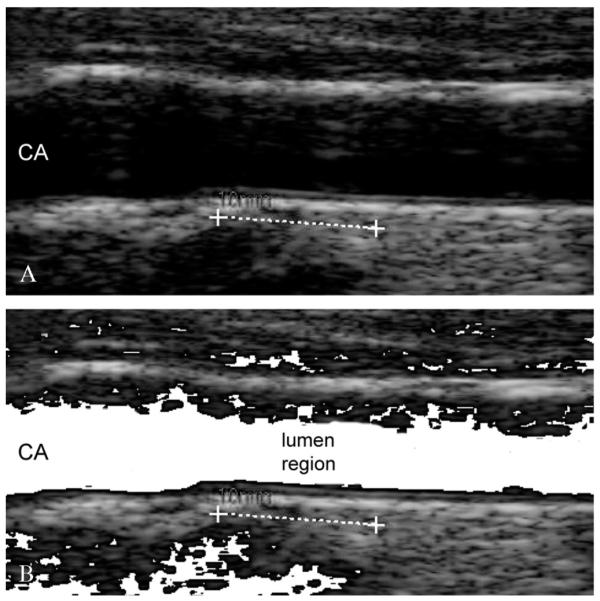
Lumen region detection. A) Original cropped image; B) lumen region detection. The pixels possibly belonging to the lumen are mapped to white.
All the pixels possibly belonging to the artery lumen were marked according to the described procedure. Then, we forced the fuzzy K-means classifier of Stage-II to classify such lumen pixels into the first cluster. This avoided the LI profile bleeding into the artery lumen in 100% of the images.
SPIKE DETECTION AND REMOVAL
Small spikes can be present in the final LI/MA profiles. Again, such spikes can be generated by noise. Since the conversion factor of our database was 0.0787 mm/pixel, an IMT of 1 mm was be equivalent to 12.7 pixels. Therefore, we defined a spike as a jump higher than 6 pixels in the LI/MA profiles, which means about half the nominal IMT value. All the spikes were detected and substituted by the average value of the 10 points neighboring the spiky point (5 points to the left and 5 to the right).
IMT measurement and performance metric
The segmentation errors were computed by comparing automated tracings by CALEX 3.0 with manual segmentations, which were traced by expert sonographers by using a custom-made research prototype available system (ImgTracer™, Global Biomedical Technologies, Inc., California, USA). We used the Polyline Distance measure (PDM) as performance metric. A detailed description of the PDM can be found in previous works.33 The fundamental equations of the PDM metric are reported in the Appendix A1. Consider that the output of the CALEX 3.0 system consists of two profiles: LI and MA. Both the profiles consist of a certain number of vertices or points on the LI/MA borders. First, we compute the average distance of the vertices of LI with respect to the segments of MA and we call this value as DLI-MA. Then, we compute the average distance between the vertices of MA with respect to the segments of LI and call such distance as DMA-LI. The PDM is defined as the sum of DLI-MA with DMA-LI divided by the total number of vertices of the two profiles. The main advantage of using the PDM as performance metric is that it is almost insensible to the number of points constituting a profile.
For each image, we compared the IMT measured by CALEX 3.0 with the IMT value calculated from manual delineations (GT). We then computed the IMT bias (i.e., the difference between CALEX 3.0 measurement and GT IMT), the IMT absolute error (i.e., the absolute difference between CALEX 3.0 measurement and GT IMT), and the IMT squared error (i.e., the squared absolute difference between CALEX 3.0 measurement and GT IMT). A detailed description of the error metrics is reported by the Appendix A2. We also computed the Figure-of-Merit (FoM) for CALEX 3.0, which corresponds to the percent agreement between the computer-estimated IMT and manually measured IMT values (mathematical details are reported in Appendix 3).
The performance evaluation analysis was completed by Bland-Altmann plots, correlation plots, and distribution histogram of the IMT measurement errors.
Results
CALEX 3.0 successfully segmented all the 885 images of the database. Table I reports the IMT measurement performance for CALEX 3.0 in comparison to Ground Truth. CALEX 3.0 measured an average IMT of 0.407±0.083 mm, whereas the GT IMT value was 0.429±0.052 mm. The IMT bias was as low as 0.022±0.081 mm, the absolute error was 0.061±0.058 mm, and the squared error was 0.007±0.015 mm2. The FoM was equal to 94.7%.
Table I.
Overall system performance for CALEX 3.0.
| CALEX 3.0 | Ground Truth | |
|---|---|---|
| IMT Mean | 0.407 ± 0.083 mm | 0.429 ± 0.052 mm |
| IMT bias | 0.022 ± 0.081 mm | - |
| IMT absolute error | 0.061 ± 0.058 mm | - |
| IMT squared error | 0.007 ± 0.015 mm2 | - |
| FoM | 94.7 % | - |
Table I clearly shows the reliability and reproducibility of the technique.
Figure 7 reports samples of CALEX 3.0 automated segmentation compared to ground truth (GT). The left column of fig. 7 shows the comparison of the LI profiles w.r.t GT, while the right column of Figure 7 shows for the MA profiles. The CALEX 3.0 profiles are depicted by continuous white lines, whereas the GT profiles by dashed lines. Figure 7 clearly demonstrates the overall agreement between automated and manual profiles.
Figure 7.

Samples of CALEX 3.0 automated segmentation (white lines) compared to manual segmentations (white dashed lines). The left column reports the lumen-intima profiles, the right the media-adventitia.
Figures from 8 to 10 depict the overall CALEX 3.0 performance. Specifically, Figure 8 reports the correlation plot between the CALEX 3.0 IMT measurements and the corresponding GT IMT values.
Figure 8.
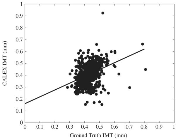
Correlation plot between CALEX 3.0 IMT values (vertical axis) and GT IMT values (horizontal axis).
Figure 9.
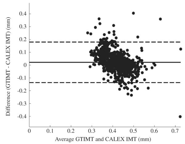
Bland-Altmann plot of the CALEX 3.0 IMT measurements compared to ground truth.
Figure 10.
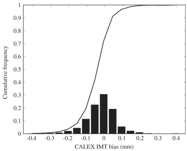
Histogram distribution of the IMT measurement bias. It can be noticed that the average IMT bias is very low and the standard deviation of the histogram is lower than 0.1 mm.
Figure 9 reports the Bland-Altmann plot for CALEX 3.0 compared to GT. Finally, Figure 10 reports the histogram distribution of the IMT measurement bias (as defined in Appendix A1). The black line on the histogram is the cumulative function. From Figure 9 it is possible to observe that CALEX 3.0 IMT error is as low as 0.022 mm (black line) with reproducibility lower than 1 mm (equal to 0.081 mm – dashed lines). This IMT measurement error was about 5% of the average IMT value on the population (manually measured as 0.429 mm – Table I). The Bland-Altmann plot (Figure 9) did not evidence any clear trend in the IMT measurement error. The distribution of the IMT error was in the range (-0.2, 0.2) mm (Figure 10), which was an index of high system reproducibility. The cumulative function of the histogram revealed that less than 7% of the images had an IMT error higher than 0.1 mm. Also, the average IMT error is centered on zero and the error distribution is symmetrical, thus evidencing that there is not a clear tendency towards under- or overestimation of the IMT value. This was an indication of high system accuracy.
The optimization of the system and the integrated architecture lowered the computational time to be about 1 s for each image. With this automated tool, therefore, we could process the 885 images of our database in less than 15 minutes.
Discussion
In this paper we showed the potential of CALEX 3.0 - an automated IMT measurement applied to an epidemiological study. This study is novel for many reasons:
It is the first time a fully automated method for carotid IMT measurement (a class of patented AtheroEdge™ systems) has been applied to an epidemiological study;
The dataset was relatively large (about 885 images) with low contrast and low-resolution.
The CALEX 3.0 is accurate and provides reproducible results.
The system takes 1 second per image and is near real time.
There is no user-interaction involved and is thus fully automated.
The system parameters are automatically and dynamically adjusted.
Our technique showed very good performance when applied to this database. The major challenge we had to face was the low pixel density of the B-Mode ultrasound images. We measured a pixel density of 12.7 pixels/mm, which led to a pixel physical dimension of 0.0787 mm/pixel (conversion factor). Since the average IMT value manually measured by an expert sonographer came out to be about 0.42 mm, it means that the IMT was represented on about 5.7 pixels in thickness. Thus it is very challenging for an automated system to find the LI/MA borders which are just 5-6 pixels apart. For example, if the IMT measurement error was of 0.5 pixels (that is a sub-pixel error), the measurement error would be of about 0.04 mm, this accounts to 10% of the average IMT value on the sample population. Our IMT measurement bias and reproducibility was 0.022 ± 0.081 mm, a nearly less than a quarter of a pixel – hence highly accurate.
From a technical point of view, CALEX 3.0 performance was satisfactory both in terms of measurement accuracy and of reproducibility. The accuracy of about 0.02 mm is in line with that of semi-automated techniques. For example, Stein et al.34 tested their semi-automated edge-based system for IMT measurement on 300 images, acquired on 25 consecutive controls and 25 consecutive patients referred to the IMT measurement by their physician. They got an error of 0.012±0.006 mm. Faita et al.35 obtained an IMT measurement bias equal to 0.01±0.038 mm and tested their semi-automated algorithm based on an edge snapper on 150 images taken from 80 healthy subjects and 70 patients with increased cardiovascular risk. Though the difference between our method and Faita et al. and Stein’s are in the range of 0.012 mm, we have to keep in mind that a great amount of user-interaction was done in these methods. Further, their techniques were fine-tuned for a specific ultrasound scanner, while CALEX 3.0 was not specifically modified in order to work with the images of this Asian Indian database.
We believe that the most important result of CALEX 3.0 was the high reproducibility of the IMT measurement. The standard deviation of the IMT bias (i.e., which is called reproducibility) was as low as 0.081 mm. Compared to Stein’s technique, which is the most reproducible method we found in literature, CALEX 3.0 could still have scope of improvement. Nevertheless, the value of one mm for reproducibility can be nowadays considered as the threshold limit for automated techniques.36 In fact, fully automated techniques need superior architecture and quality controls in order to optimize the IMT computation with respect to the semi-automated and user-driven techniques, and the lack of such controls increases the IMT bias standard deviation (thus lowering reproducibility).
Finally, CALEX 3.0 is an IMT automated measurement paradigm that has been integrated into a versatile and commercial platform called AtheroEdge™ (Global Biomedical Technologies, Inc., CA, USA).
Conclusions
We demonstrated the usage of AtheroEdge™ class of system on a low contrast and low resolution (pixel density was 12.7 pixels/mm) epidemiological study consisting of a database of 885 carotid ultrasound images. The CALEX 3.0 fully automated system processed 100% of the images in the dataset and shows an IMT measurement bias (compared to human tracings) of 0.022±0.081 mm, comparable to previous semi-automated methods on accuracy and reproducibility. Thus CALEX 3.0 can therefore be used in large multi-centric and epidemiological studies involving low-resolution imaging acquired by low-end ultrasound equipments.
Acknowledgements
The Hyderabad DXA Study was funded by the Wellcome Trust (WT083707MA).
Appendix.
A1. PolyLine Distance
The polyline distance metric (PDM) is a robust metric to define the distance between two boundaries. The basic idea is to measure the distance of each vertex of a boundary to the segments of the other boundary. The polyline distance from vertex ν to the boundary B2 can be defined as the minimum distance between ν and the segments of B2. The distance between the vertexes of B1 to the segments of B2 is then defined as the sum of the distances from the vertexes of B1 to the closest segment of B2. Let’s call this distance as d(B1, B2). Similarly, it is possible to calculate the distance between the vertices of B2 to the closest segment of B1 (let’s call this distance as d(B1, B2)). The polyline distance between boundaries is then defined as:
| (1) |
A2. Definition of the IMT bias, absolute error, and squared errors
Let IMTi be the intima-media thickness value automatically computed by CALEX 3.0 on the i-th image of the database. Let GTIMTi be the IMT value computed by manual measurements.
The IMT measurement bias εi is defined as:
| (2) |
The absolute value μi of the IMT bias is defined as:
| (3) |
The squared error ηi is, finally, defined as:
| (4) |
By averaging all these error metrics on the N images of the database, we computed the overall system errors as:
| (5) |
| (6) |
| (7) |
A3. Figure-of-Merit
Let IMTi be the intima-media thickness value automatically computed by CALEX 3.0 on the i-th image of the database. Let GTIMTi be the IMT value computed by manual measurements. If we consider a database of N images, then the overall system IMT estimate can be defined as:
| (8) |
| (9) |
The Figure-of-Merit (FoM) is mathematically represented as:
| (10) |
References
- 1.Organization WH [cited 2011, Oct 12];Cardiovascular disease [Internet] Available from http://www.who.int/cardiovascular_diseases/en/
- 2.Badimon JJ, Ibanez B, Cimmino G. Genesis and dynamics of atherosclerotic lesions: implications for early detection. Cerebrovasc Dis. 2009;27(Suppl 1):38–47. doi: 10.1159/000200440. [DOI] [PubMed] [Google Scholar]
- 3.Walter M. Interrelationships among HDL metabolism, aging, and atherosclerosis. Arterioscler Thromb Vasc Biol. 2009;29:1244–50. doi: 10.1161/ATVBAHA.108.181438. [DOI] [PubMed] [Google Scholar]
- 4.Kampoli AM, Tousoulis D, Antoniades C, Siasos G, Stefanadis C. Biomarkers of premature atherosclerosis. Trends Mol Med. 2009;15:323–32. doi: 10.1016/j.molmed.2009.06.001. [DOI] [PubMed] [Google Scholar]
- 5.JM UK-I, Young V, Gillard JH. Carotid-artery imaging in the diagnosis and management of patients at risk of stroke. Lancet Neurol. 2009;8:569–80. doi: 10.1016/S1474-4422(09)70092-4. [DOI] [PubMed] [Google Scholar]
- 6.Kastelein JJ, Wiegman A, de Groot E. Surrogate markers of atherosclerosis: impact of statins. Atheroscler Suppl. 2003;4:31–6. doi: 10.1016/s1567-5688(03)00007-2. [DOI] [PubMed] [Google Scholar]
- 7.Polak JF, Pencina MJ, Meisner A, Pencina KM, Brown LS, Wolf PA, et al. Sr. Associations of Carotid Artery Intima-Media Thickness (IMT) With Risk Factors and Prevalent Cardiovascular Disease: Comparison of Mean Common Carotid Artery IMT With Maximum Internal Carotid Artery IMT. J Ultrasound Med. 2010;29:1759–68. doi: 10.7863/jum.2010.29.12.1759. [DOI] [PMC free article] [PubMed] [Google Scholar]
- 8.Touboul PJ, Hennerici MG, Meairs S, Adams H, Amarenco P, Bornstein N, et al. Mannheim carotid intima-media thickness consensus (2004-2006). An update on behalf of the Advisory Board of the 3rd and 4th Watching the Risk Symposium, 13th and 15th European Stroke Conferences, Mannheim, Germany, 2004, and Brussels, Belgium, 2006. Cerebrovasc Dis. 2007;23:75–80. doi: 10.1159/000097034. [DOI] [PubMed] [Google Scholar]
- 9.Touboul PJ, Hennerici MG, Meairs S, Adams H, Amarenco P, Desvarieux M, et al. Mannheim intima-media thickness consensus. Cerebrovasc Dis. 2004;18:346–9. doi: 10.1159/000081812. [DOI] [PubMed] [Google Scholar]
- 10.Watanabe H, Yamane K, Egusa G, Kohno N. Influence of westernization of lifestyle on the progression of IMT in Japanese. J Atheroscler Thromb. 2004;11:330–4. doi: 10.5551/jat.11.330. [DOI] [PubMed] [Google Scholar]
- 11.van der Meer IM, Bots ML, Hofman A, del Sol AI, van der Kuip DA, Witteman JC. Predictive value of noninvasive measures of atherosclerosis for incident myocardial infarction: the Rotterdam Study. Circulation. 2004;109:1089–94. doi: 10.1161/01.CIR.0000120708.59903.1B. [DOI] [PubMed] [Google Scholar]
- 12.Liu L, Zhao F, Yang Y, Qi LT, Zhang BW, Chen F, et al. The clinical significance of carotid intima-media thickness in cardiovascular diseases: a survey in Beijing. J Hum Hypertens. 2008;22:259–65. doi: 10.1038/sj.jhh.1002301. [DOI] [PubMed] [Google Scholar]
- 13.Beneficial effect of carotid endarterectomy in symptomatic patients with high-grade carotid stenosis. North American Symptomatic Carotid Endarterectomy Trial Collaborators. N Engl J Med. 1991;325:445–53. doi: 10.1056/NEJM199108153250701. [DOI] [PubMed] [Google Scholar]
- 14.Fisher M, Martin A, Cosgrove M, Norris JW. The NAS-CET-ACAS plaque project. North American Symptomatic Carotid Endarterectomy Trial. Asymptomatic Carotid Atherosclerosis Study. Stroke. 1993;24:I24–5. discussion I31-2. [PubMed] [Google Scholar]
- 15.Grogan JK, Shaalan WE, Cheng H, Gewertz B, Desai T, Schwarze G, et al. B-mode ultrasonographic characterization of carotid atherosclerotic plaques in symptomatic and asymptomatic patients. J Vasc Surg. 2005;42:435–41. doi: 10.1016/j.jvs.2005.05.033. [DOI] [PubMed] [Google Scholar]
- 16.Johnsen SH, Mathiesen EB. Carotid plaque compared with intima-media thickness as a predictor of coronary and cerebrovascular disease. Curr Cardiol Rep. 2009;11:21–7. doi: 10.1007/s11886-009-0004-1. [DOI] [PubMed] [Google Scholar]
- 17.Bhuiyan AR, Srinivasan SR, Chen W, Paul TK, Berenson GS. Correlates of vascular structure and function measures in asymptomatic young adults: the Bogalusa Heart Study. Atherosclerosis. 2006;189:1–7. doi: 10.1016/j.atherosclerosis.2006.02.011. [DOI] [PubMed] [Google Scholar]
- 18.Schargrodsky H, Hernandez-Hernandez R, Champagne BM, Silva H, Vinueza R, Silva Aycaguer LC, et al. CAR-MELA: assessment of cardiovascular risk in seven Latin American cities. Am J Med. 2008;121:58–65. doi: 10.1016/j.amjmed.2007.08.038. [DOI] [PubMed] [Google Scholar]
- 19.de Groot E, van Leuven SI, Duivenvoorden R, Meuwese MC, Akdim F, Bots ML, Kastelein JJ. Measurement of carotid intima-media thickness to assess progression and regression of atherosclerosis. Nat Clin Pract Cardiovasc Med. 2008;5:280–8. doi: 10.1038/ncpcardio1163. [DOI] [PubMed] [Google Scholar]
- 20.Rothwell PM, Gibson RJ, Slattery J, Warlow CP. Prognostic value and reproducibility of measurements of carotid stenosis. A comparison of three methods on 1001 angiograms. European Carotid Surgery Trialists’ Collaborative Group. Stroke. 1994;25:2440–4. doi: 10.1161/01.str.25.12.2440. [DOI] [PubMed] [Google Scholar]
- 21.Naqvi TZ. Ultrasound vascular screening for cardiovascular risk assessment. Why, when and how? Minerva Cardioangiol. 2006;54:53–67. [PubMed] [Google Scholar]
- 22.Sipila O, Blomqvist P, Jauhiainen M, Kilpelainen T, Malaska P, Mannila V, et al. Reproducibility of phantom-based quality assurance parameters in real-time ultrasound imaging. Acta Radiol. doi: 10.1258/ar.2011.100227. [DOI] [PubMed] [Google Scholar]
- 23.Lieu D. Ultrasound physics and instrumentation for pathologists. Arch Pathol Lab Med. 134:1541–56. doi: 10.5858/2009-0730-RA.1. [DOI] [PubMed] [Google Scholar]
- 24.Loizou CP, Pattichis CS, Pantziaris M, Tyllis T, Nicolaides A. Quality evaluation of ultrasound imaging in the carotid artery based on normalization and speckle reduction filtering. Med Biol Eng Comput. 2006;44:414–26. doi: 10.1007/s11517-006-0045-1. [DOI] [PubMed] [Google Scholar]
- 25.Molinari F, Zeng G, Suri JS. An integrated approach to computer-based automated tracing and its validation for 200 common carotid arterial wall ultrasound images: A new technique. J Ultras Med. 2010;29:399–418. doi: 10.7863/jum.2010.29.3.399. [DOI] [PubMed] [Google Scholar]
- 26.Molinari F, Zeng G, Suri JS. Intima-media thickness: setting a standard for completely automated method for ultrasound. IEEE Transaction on Ultrasonics Ferroelectrics and Frequency Control. 2010;57:1112–24. doi: 10.1109/TUFFC.2010.1522. [DOI] [PubMed] [Google Scholar]
- 27.Molinari F, Liboni W, Giustetto P, Badalamenti S, Suri JS. Automatic computer-based tracings (ACT) in longitudinal 2-D ultrasound images using different scanners. Journal of Mechanics in Medicine and Biology. 2009;9:481–505. [Google Scholar]
- 28.Molinari F, Zeng G, Suri J. Greedy technique and its validation for fusion of two segmentation paradigms leads to an accurate intima-media thickness measure in plaque carotid arterial ultrasound. The Journal for Vascular Ultrasound. 2010;34:63–73. [Google Scholar]
- 29.Molinari F, Zeng G, Suri J. Inter-Greedy Technique for Fusion of Different Segmentation Strategies Leading to High-Performance Carotid IMT Measurement in Ultrasound Images. Journal of Medical Systems. 2010:1–15. doi: 10.1007/s10916-010-9507-y. [DOI] [PubMed] [Google Scholar]
- 30.Saba L, Montisci R, Molinari F, Tallapally N, Zeng G, Mallarini G, Suri JS. Comparison between manual and automated analysis for the quantification of carotid wall by using sonography. A validation study with CT. Eur J Radiol. doi: 10.1016/j.ejrad.2011.02.047. (in press) [DOI] [PubMed] [Google Scholar]
- 31.Saba L, Sanfilippo R, Tallapally N, Molinari F, Montisci R, Mallarini G, Suri JS. Evaluation of carotid wall thickness by using Computed Tomography (CT) and semi-automated ultrasonographic software. Journal for Vascular Ultrasound. (in press) [Google Scholar]
- 32.Molinari F, Zeng G, Suri JS. 2010 AIUM Annual Convention. San Diego, CA, USA: 2010. Effect of learning algorithm on automated tracigns of adventitia borders in atherosclerotic common carotid artery (CCA) ultrasound. [Google Scholar]
- 33.Suri JS, Haralick RM, Sheehan FH. Greedy algorithm for error correction in automatically produced boundaries from low contrast ventriculograms. Pattern Anal Appl. 2000;3:39–60. [Google Scholar]
- 34.Stein JH, Korcarz CE, Mays ME, Douglas PS, Palta M, Zhang H, et al. A semiautomated ultrasound border detection program that facilitates clinical measurement of ultrasound carotid intima-media thickness. J Am Soc Echocardiogr. 2005;18:244–51. doi: 10.1016/j.echo.2004.12.002. [DOI] [PubMed] [Google Scholar]
- 35.Faita F, Gemignani V, Bianchini E, Giannarelli C, Ghiadoni L, Demi M. Real-time measurement system for evaluation of the carotid intima-media thickness with a robust edge operator. J Ultrasound Med. 2008;27:1353–61. doi: 10.7863/jum.2008.27.9.1353. [DOI] [PubMed] [Google Scholar]
- 36.Molinari F, Zeng G, Suri JS. A state of the art review on intima-media thickness (IMT) measurement and wall segmentation techniques for carotid ultrasound. Computer Methods and Programs in Biomedicine. 2010;100:201–21. doi: 10.1016/j.cmpb.2010.04.007. [DOI] [PubMed] [Google Scholar]