The Effect of Ionic Strength on the Mechanical, Structural and Transport Properties of Peptide Hydrogels

Abstract

It is found that the elastic modulus of a peptide hydrogel increases linearly with the logarithm of its ionic strength. This result indicates that the elastic modulus of this class of hydrogels can be tuned by the ionic strength in a highly predictable manner. Small-angle X-ray scattering studies reveal that higher ionic strength leads to thinner but more rigid peptide fibers that are packed more densely. The self-diffusion coefficient of small molecules inside the hydrogel decrease linearly with its ionic strength, but this decrease is mainly a salt effect rather than diffusion barriers imposed by the hydrogel matrix.

Introduction

Hydrogels are viscoelastic materials which can find use in tissue engineering, cell culture and drug delivery.^1-5 For these applications, the mechanical and transport properties of the hydrogels are important considerations. Mechanical properties are important not just for structural support purposes, but also for functional purposes. For example, shear-responsiveness is required for injectable hydrogels.⁶ Another example is that stem cell specification is very sensitive to the elasticity of the hydrogel matrix.^{7, 8} Transport properties are important because nutrients and metabolites need to pass through and drugs should have their diffusion retarded in a controlled manner. For these reasons, the mechanical and transport properties of hydrogels have been extensively investigated.^{6, 9-14}

Ionic strength is an effective way to induce hydrogelation and to modulate hydrogel properties, including mechanical and transport properties.^9,15-17 In synthetic hydrogels, it is often observed that the elastic modulus of the hydrogel, G’, increases with ionic strength. For example, Schneider and Pochan found that when the ionic strength of a peptide hydrogel increased from 20 to 400 mM, the elastic modulus G’ increased from 100 Pa to 3000 Pa.¹⁶ Skouri and co-workers reported that the shear modulus of poly(acrylic acid) gel increases with the addition of salt and the authors attributed this effect to the screening of the electrostatic repulsions.¹⁸ In a nanocomposite hydrogel formed by Laponite and poly(ethylene oxide), Schexnailder and co-workers observed a linear increase of the elastic modulus G’ from 0.8 to 1.7 kPa as the concentration of added NaCl increased from zero to 0.1 M. The authors attributed this phenomenon to increased heterogeneity in the spatial distribution of the nanoparticles (Laponite) and the polymers (PEO).¹⁹

Hydrogels extracted from animal sources often display a trend opposite of synthetic hydrogels. For example, Johnson et al. observed that the elastic modulus G’ of a hydrogel extracted from porcine myocardial tissue decreased to 1/2~1/3 of its original value when the ionic strength increased from 0.5×PBS to 1.5×PBS.²⁰ The authors implied that ionic strength impacts fibrillogenesis, which leads to changes in G’. Jin and Grodzinsky found that the elastic modulus G’ of bovine calf cartilage decreased monotonically when the NaCl concentration in the surrounding bath increased from 0.01 to 1.0 M.²¹ They assumed that the elastic modulus of cartilage tissue has two contributions, electrical and nonelectrical. NaCl screens the electrical contribution, thus decreasing the elastic modulus.

To achieve a better understanding of the ionic strength effect of on hydrogel elasticity, it is imperative that a wide ionic strength range is covered. To this end, we use a pair of oppositely charged oligopeptides which co-assemble into hydrogels upon mixing.⁹ Unlike self-assembling peptides where slight variation in ionic strength can induce hydrogelation, in the co-assembling system each individual peptide solution can withstand large ionic strength variation without undergoing gelation. This allows us to study gelation over a wide ionic strength range (0.1 – 2.1 M in this work). Further, such mixing-induced gelation allows precise control of the pH and the ionic strength of the hydrogels.

To gain a mechanistic understanding of how ionic strength impacts hydrogel elasticity, we integrate mechanical studies with structural studies in this work. Gelation is monitored in parallel by dynamic rheometry, which provides mechanical information, and small-angl e X-ray scattering (SAXS), which provides structural information. Additionally, the diffusion of small molecules inside the hydrogels is assessed by NMR spectroscopy.

Materials and methods

Peptide design and synthesis

Two undecapeptides, E11 and K11 (Table 1), were designed based on our previous work.²² E11 carries negative charges at pH 7.4, while K11 is positively charged under the same condition. The N- and C-terminal blockage produces neutral ends in both peptides, which simplify electrostatic interactions between the peptide pair. Each peptide contains two tryptophans. The motivation is to strengthen the hydrogel through the stacking of aromatic side chains positioned at the terminals of the peptides. It has been reported that aromatic residues can promote hydrogelation of oligopeptides through stacking.²³ And at the same time, the UV absorption of the tryptophan residues at 280 nm could be used to measure peptide concentration in solution.²⁴

Table 1.

Sequences and molecular weights (M.W.) of a pair of undecapeptides E11 and K11.^a

Gelators	peptides	sequences	M. W. (Da)
A	E11	acetyl-Glu-Trp-Glu-Ala-Glu-Ala- Glu-Ala-Glu-Trp-Glu-amide	1,419
B	K11	acetyl-Lys-Trp-Lys-Ala-Lys-Ala- Lys-Ala-Lys-Trp-Lys-amide	1,413

^aAla, alanine; Glu, glutamic acid; Lys, lysine; Trp, tryptophan. The N-and C-termini of each peptide were acetylated (acetyl-) and amidated (-amide), respectively.

The peptides were synthesized on Rink-amide MBHA (aapptec Inc., USA) resin using a CEM microwave synthesizer with standard Fmoc-chemistry method.²⁵ The N-terminal of each peptide was acetylated by acetic anhydride. After cleavage by a TFA cocktail (TFA/TIS/water, 95/2.5/2.5, volume ratio), the crude peptide was purified by reverse-phase HPLC method. The final products were characterized by mass spectrometry and analytical HPLC. (ESI)

Peptide stock solution preparation

For NMR measurements, all peptide solutions were prepared in D₂O buffers so that the peptide ¹H signals can be observed with little background interference. This also prevents the ¹H₂O signal from overflowing the spectrometer receiver when determining water diffusion coefficient (D₂O contains trace amount of H₂O). To facilitate comparison of results from different methods, peptide samples for rheological and SAXS measurements were also prepared in D₂O buffers.

Stock solutions containing 32 mM E11 or K11 peptide was prepared in 50 mM sodium phosphate in D₂O. This stock solution also contains 16 mM 4,4,4-trifluorophenylalanine (tfF, from Chem-impex, Inc. USA). tfF is used as a probe to evaluate small molecule diffusion inside hydrogels.¹¹ The advantage of using tfF is that its diffusion can be measured through the ¹⁹F signal without interference from the peptide gelators. Peptide concentration was determined based on the UV absorption of Trp (ε₂₈₀ = 5690 M⁻¹·cm⁻¹).²⁴ tfF concentration was determined based on weight. tfF has no interference with the UV absorption of Trp at 280 nm. The pH of the stock solution was adjusted to 7.4 using NaOH or HCl (without pD correction). To make solutions of different ionic strength, 50 mM sodium phosphate solutions containing 0, 0.2, 1.0, 2.0 and 4.0M NaCl were prepared, also at pH 7.4 (without pD correction). The 32 mM peptide stock solution was then mixed with equal volume of NaCl solution to obtain solutions containing 16 mM peptide gelator (E11 or K11), 8 mM tfF, 50 mM sodium phosphate, and NaCl of various concentrations: 0, 0.1, 0.5, 1.0 and 2.0 M. The five E11 solutions are denoted as A-1, A-2, A-3, A-4 and A-5, respectively, while the five K11 solutions are denoted as B-1, B-2, B-3, B-4 and B-5, respectively (Table 2). Solution A-i is mixed with solution B-i to form hydrogel Gel-i (i =, 1, 2, 3, 4, and 5). Note that in SAXS samples, tfF was not added to minimize background scattering. The ionic strength (μ) of each hydrogel is calculated as below:

$$\mu =\frac{1}{2}\underset{i=1}{\overset{n}{\Sigma }}{c}_i{Z_i}^2$$ (1)

where c_i is the molar concentration of the i-th ion (in M), Z_i is the charge number of that ion, and the sum is taken over all the ions in the solution. This includes contributions from sodium phosphate (50 mM) and NaCl (various concentrations). However, peptides are not included in ionic strength calculation since in the gelled state there is hardly any free peptide left.²² tfF is also not included in the ionic strength calculation since it is a zwitterion with a net charge of zero. To dispel doubt about this practice, the actual conductivity of each peptide solution was measured prior to mixing (Table 2). Experimental results will be analyzed both in terms of hydrogel ionic strength (μ) and solution conductivity (Λ).

Table 2.

Composition and conductivity (Λ) of peptide solutions and ionic strength of the hydrogels.^a

Hydrogels	Gel-1 (0.1 M)		Gel-2 (0.2 M)		Gel-3 (0.6 M)		Gel-4 (1.1 M)		Gel-5 (2.1 M)
Gelator sol.	A-1	B-1	A-2	B-2	A-3	B-3	A-4	B-4	A-5	B-5
E11 (mM)	16	0	16	0	16	0	16	0	16	0
K11 (mM)	0	16	0	16	0	16	0	16	0	16
NaCl (M)	0	0	0.1	0.1	0.5	0.5	1.0	1.0	2.0	2.0
Λ (mS·cm−1)	8.8	8.7	15.9	16.0	41.0	40.9	76.2	75.9	122.7	122.5

^aHydrogel Gel-i is made by mixing two peptide solutions A-i and B-i (i = 1, 2, 3, 4, and 5). In addition to the peptide and NaCl, each peptide solution also contains 8 mM tfF and 50 mM sodium phosphate. The conductivity of each peptide solution was measured by a conductivity meter at r.t; the ionic strength of each hydrogel (in the parentheses) was calculated using Eqn. 1.

In NMR experiments, five control solutions of pH 7.4 were also made. These control solutions have the same composition as the hydrogels except peptides: each control solution contains 50 mM sodium phosphates, 8 mM tfF, and the same amount NaCl as the corresponding hydrogel.

UV and NMR spectroscopy studies indicate that even at the highest ionic strength (2.1 M), there is no peptide aggregation (see Figures S4-S6 in ESI). This is the benefit obtained by separating the positive and negative charges into separate modules. Note that in oligopeptides with similar sequences but where the positive and negative charges reside in the same peptide, slight elevation of the ionic strength (< 5 mM) can induce gelation.²⁶

Rheological experiments

All hydrogels (Gel-1 to Gel-5) were prepared and measured at 25 °C. The peptide solutions were prepared as described above. To prepare hydrogel Gel-i, gelator solutions A-i and B-i were centrifuged separately for 10 min at 8,000 rpm followed by degassing at house vaccum (1–2 min at 21 Torr). Centrifugation is necessary to remove any suspended impurities which might cause the inhomogeneous gelation. Degassing helps to remove excess gases from the solutions otherwise capable to form bubbles during gelation and affect the formation of hydrogels and the results. 200 μL of each A-i and B-i solutions were mixed through a Y-shaped connector in the sealed cell of the rheometer. Rheological measurements started immediately after the sample is loaded.

Dynamic rheological measurements were performed using a NOVA Rheometer (REOLOGICA Instruments, Inc., Sweden) with a null balance system which allows for nano-torque and nano-strain measurement and analysis. The instrument is also equipped with a sealed-cell geometry which prevents dehydration of water-based samples during prolonged measurements. In addition, to exclude possible dehydration of the samples at 25 °C, a simple in-house designed system was used to humidify the incoming air used for the sealed-cell bearing. Rheological characterizations of the samples were performed using a 25 mm diameter cone-and-plate steel geometry (4° angle). Detailed descriptions of the rheological measurements can be found elsewhere.²⁷ Briefly, time-sweep measurements were conducted at 0.2% strain amplitude and 1 rad/s angular frequency. Time-sweep was followed by frequency-sweep at 0.2% strain amplitude, with the angular frequency varying from 0.01 to 100 rad/s in a log mode with 18 data points per frequency decade (not shown). After frequency-sweep but before strain-sweep, a time-sweep of 3 h was performed on each hydrogel at 0.2 % strain amplitude, 1 rad/s angular frequency to confirm that the gel remains undisturbed by the frequency-sweep (see ESI). Strain-sweep measurements were then performed with a single integration cycle at 1 rad/s angular frequency, within the range of strain amplitudes varying from 0.1% to 100% in a log mode with 23 data points per decade.

Small Angle X-ray Scattering (SAXS) experiments

Peptide solutions were prepared as described above. To prepare hydrogels for SAXS experiments, equal volumes of each peptide solution (10-15 μL) were centrifuged (20 sec at 500 RPM) into a cylindrical glass capillary (Charles Supper Co.) with a diameter of 1.0 mm and a wall thickness of 0.01 mm. Scattering data were collected at 0.5, 1.5, 3, 5, 7, 24, 48, and 72 h after mixing for Gel-1 – Gel-5.

SAXS data were collected using the beamline 12ID-B of the Advanced Photon Sources (APS) at the Argonne National Laboratory. For every measurement, the monochromic X-ray beam (λ = 0.689 Å) with a cross-section size of 0.07 mm × 0.20 mm was adjusted to pass through the centers of the capillaries. The exposure time for all samples was set to 0.2 sec to avoid detector saturation and radiation damage to the samples. X-ray scattering intensities were collected using the 2D detector Pilatus 2M (DECTRIS Ltd). The 2D scattering images were converted into 1D scattering profiles of I(Q) vs. Q in the Q-range from 0.007 Å⁻¹ to 0.6 Å⁻¹ by means of azimuthal averaging after solid angle correction. The resulting 1D profiles were normalized over the intensity of the transmitted X-ray beam, using the software package at the beamline 12ID-B. I(Q) is the scattering intensity of X-rays, and Q is the scattering vector amplitude which is related to the X-ray wavelength λ and the scattering angle θ by Eqn. (2):

$$Q=\frac{4\pi }{\lambda }\sin (\theta ∕2)$$ (2)

Subtraction of the solvent scattering involved normalization based on the ratio of incident and transmitted X-ray photon counts. This is to account for the slight differences in capillary thickness. Additional background scattering correction was performed in accordance with the generally accepted published procedure.²⁸ The SAXS instrument has a pinhole geometry and the high flux of the X-ray beam from the synchrotron reduced the data collection time down to 0.2 sec, thus allowing the use of SAXS to monitor the gelation process in real time.

Model functions for IGOR Pro 6.2 developed by the NIST Center of Neutron Research²⁹ were used to analyze the persistence length of the fibers underlying Gel-1 – Gel-5. The persistence length L_p is obtained from the simulations of semi-flexible worm-like chain model where an individual hydrogel fiber is approximated by the chain of connected locally stiff segments of length L_p.³⁰ For simplicity, these locally stiff segments are approximated by cylinders. The persistence length L_p is the length over which the cylinder could be considered a rigid rod.^{30, 31}

The ATSAS software^{32, 33} PRIMUS was used to estimate the zero-angle scattering intensity I(0) from the Guinier analysis of lnI(Q) vs. Q² plots. Since I(0) characterizes the mass of the scattering particles, it was used to monitor the gelation process of all hydrogels over time. The linearity of Guinier plots for rod like particles lnQI(Q) vs. Q² suggests that the fibers in Gel-1 – Gel-5 have one dimension (length) much longer than the other two. This longest dimension is beyond the resolution limit (Q_min) of the scattering data (in our case Q_min ~ 0.007 Å⁻¹ which means the maximum dimension we can reliably characterized is ~500 Å). We therefore analyzed the scattering data in terms of the cross-sections of the scattering particles. This is achieved by multiplying I(Q) by Q, a procedure that effectively removes information about the longest dimension (length) of the scattering particle.³⁴ A simulated annealing algorithm used for restoring the 3D shape of scattering objects,³⁵ was used to restore the 2D cross-sections for Gel-1 – Gel-5. Here, we model the 2D cross-sections of the fibers formed by Gel-1 – Gel-5 using the algorithm in a purpose-written program that is described elsewhere.³⁶ In SAXS data processing, the spherical dummy atoms were arranged on a flat grid of 20 × 20 close-packed dummy atoms, each 3 Å in diameter. The program calculated the pair distance distribution function, P_c(r), for the model cross-section composed of the dummy atoms. P_c(r) is the distribution of distances between two random area elements in the cross-section, weighted by the scattering density at each radial distance, r. The optimization procedure is in general described elsewhere.^{28, 34} After optimization, the radius of gyration of the cross-section R_c and the maximum cross-sectional dimension dmax, both in Å, were determined from P_c(r). The second moment of P_c(r) yields R_c, which is the contrast-weighted mean distance of all area elements from the center of scattering density. d_max is the r value at which P_c(r) goes to 0. The program also outputs the model cross-sections as atomic coordinate files in the Protein Data Bank format which allowed their pictorial presentation. Corrections for scaling and incoherent background were applied to the model scattering profile so it could be compared directly with experimental scattering data.³⁴

Similar two-dimensional approach was used to compare the cross-sectional correlation length L_c of Gel-1 – Gel-5. 2D scattering data (QI(Q) vs. Q) were processed using the IGOR Pro 6.2/IRENA software³⁷ to estimate the cross-sectional mesh size of the cross-linking networks in the hydrogels, by means of the Debye-Bueche model³⁸ in the following form:

$$I\left(Q\right)\propto \frac{L_c^3}{{(1+Q^2{L}_c^2)}^2}$$ (3)

where L_c is the cross-sectional correlation length, which provides a measure of the spatial extent of the cross-linking regions in the imaginary plane cross-cutting the fibrous network and reflects the average cross-sectional mesh size. Larger cross-sectional correlation length correlates with larger average cross-sectional mesh size.³⁹

NMR experiments

In NMR experiments, gelator solutions A-i and B-i (see Table 2), 250 μL each, were mixed in a 1.5 mL centrifuge tube and then quickly transferred to a 5-mm NMR tube as shown in Figure 1. All the NMR experiments were carried out on a Varian INOVA 500 MHz spectrometer, equipped with a ¹H/¹⁹F/{¹³C/¹⁵N} 5-mm triple resonance probe. BPP-LED⁴⁰ technique was used to monitor the diffusion coefficients of H₂O and tfF. The self-diffusion coefficient D was extracted from the experimental data using the following equation:⁴⁰

$$A=A_0\cdot \exp (-{\gamma }^2{g}^2{\delta }^{2}D(\Delta -\delta ∕3))$$ (4)

where A and A₀ are the signal amplitude at gradient g and the initial signal amplitude (without gradient), respectively. γ is the gyromagnetic ratio (267.5 × 10⁶ rad·s⁻¹·T⁻¹ for ¹H, and 251.7 × 10⁶ rad·s⁻¹·T⁻¹ for ¹⁹F). g is strength of the pulsed-gradient, δ is the pulsed-gradient width and Δ is the diffusion time. D is the self-diffusion coefficient. In D_tfF measurement, the gradient changed from 0.018 to 0.430 T·m⁻¹ in 24 steps, Δ was set to 0.002 s, Δ was set to 0.1 s. In the D_water measurement, the gradient changed from 0.018 to 0.219 T·m⁻¹ in 12 steps, with Δ = 0.002 s and Δ = 0.1 s.

Fig. 1.

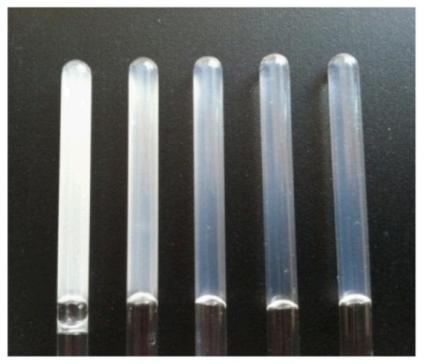
Photos of hydrogels of different ionic strength (μ). From left to right, Gel-1 (μ = 0.1 M), Gel-2 (μ = 0.2 M), Gel-3 (μ = 0.6 M), Gel-4 (μ = 1.1 M), and Gel-5 (μ = 2.1 M).

Results and discussion

Physical appearance

Figure 1 shows the physical appearance of Gel-1 to Gel-5 in 5-mm NMR tubes. All the samples formed a hydrogel which can hold its own weight. As the ionic strength increases, the hydrogel becomes increasingly transparent. Such visual observation indicates that these hydrogels are likely to have very different mechanical and structural properties.

Ionic Strength Effect on the Mechanical Properties of Hydrogels

Figure 2 shows the time- and strain-sweep results of the gelation process at different ionic strength. As the ionic strength increased from 0.1 to 2.1 M, the plateau G’ value increases more than 12 times, from 7.6 kPa (Gel-1) to 94.6 kPa (Gel-5). The plateau G’ value of the hydrogel was obtained by averaging the G’ values taken during last hour of the gelation process.

Fig. 2.

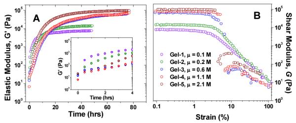
Time-sweep (A) and strain-sweep (B) of Gel-1 to Gel-5. Violet: Gel-1 (μ = 0.1 M), green: Gel-2 (μ = 0.2 M), blue: Gel-3 (μ = 0.6 M), red: Gel-4 (μ = 1.1 M), brown: Gel-5 (μ = 2.1 M). The inset in (A) shows the gelation process in its first 4 h. From (B), the strain yield value γ slightly increases from ~2% to ~4% with the increase of the ionic strength from 0.1 to 2.1 M.

When the plateau G’ values are plotted against lnμ and lnΛ, a linear dependency is observed in both cases (Figure 3). The agreement between ionic strength and conductivity plots indicate that either one can be used to analyze experimental data. This linear relationship between G’ and lnμ shows that the stiffness of this class of peptide hydrogels can be tuned by the ionic strength in a highly predictable manner.

Fig. 3.

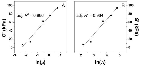
The elastic modulus G| vs. the logarithm of ionic strength (A) and logarithm of conductivity (B). μ is in M and Λ is in mS·cm⁻¹. The solid line represents linear fitting, and the goodness of fitting (adjusted R²) is labeled. The slope and intercept of linear fitting in panel A is 30.76 kPa and 73.20 kPa, respectively; the slope and intercept of linear fitting in panel B is 35.04 kPa and −73.55 kPa, respectively.

Previously, a linear dependency of G’ on μ was reported for the Laponite and poly(ethylene oxide) nanocomposite hydrogel in the NaCl concentration range of 0 – 0.1 M.¹⁹ Considering that the current work covers a much wider NaCl concentration range (0 – 2 M), the previously observed linear dependency of G’ on μ might be a limiting case of the linear dependency of G’ on lnμ. While the plateau G’ value increases monotonously with the ionic strength μ, the growth of G’ displays a more complex pattern. As μ increases from 0.1 M to 1.1 M, the growth of G’ slows down, in the order of Gel-1 > Gel-2 > Gel-3 > Gel-4 (Figure 2A inset). However, when μ further increases to 2.1 M, there is a rebound in the growth of G’ and Gel-5 is faster than Gel-3 and Gel-4. Hence the overall order of gelation speed has the following order: Gel-1 > Gel-2 > Gel-5 > Gel-3 > Gel-4.

The co-assembly of the negatively charged E11 peptide and the positively charged K11 peptide into hydrogels is mainly driven by three forces: electrostatic attractions between oppositely charged amino acids (Lys and Glu), hydrophobic interactions between neutral amino acids (Trp and Ala), and hydrogen bonding between peptide backbones.¹⁵ High ionic strength screens electrostatic attractions but enhances hydrophobic interactions. Specifically, variation of the ionic strength of the media will result in significant changes of the Debye screening length, κ⁻¹.⁴¹

$${\kappa }^{-1}={\left(\frac{{\epsilon }_r{\epsilon }_0{k}_{B}T}{2N_A{e}^2\mu }\right)}^{1∕2}$$ (5)

where κ is the Debye-Hückel reciprocal thickness, in m; ε_r is the vacuum permittivity, 8.85×10⁻¹² C²·N⁻¹·m⁻²; ε₀ is the dielectric constant of a solvent, for water at 298 K, ε₀ = 78.54; k_B is the Boltzmann constant, 1.38×10⁻²³ N·m·K⁻¹; T is the absolute temperature, 298 K; e is the elementary charge, 1.602×10⁻⁹ C; N_A is the Avogadro number, 6.022×10²³ mol⁻¹; and μ is the ionic strength of the sample, in mol·m⁻³. In our case, the Debye screening length defines the distance over which the electrostatic attraction is effective. Indeed, the estimates using eq. (5) show that within the range of our ionic strength values, significant changes in the Debye screening length could be expected—substituting 0.1 M, 0.2 M, 0.6 M, 1.1 M and 2.1 M into eq. (5) results in consistent drop in κ⁻¹ values from 9.6 Å, 6.8 Å. 3.9 Å, 2.9 Å, to 2.1 Å, respectively.

At lower ionic strength, the Debye screening length κ⁻¹ is longer, and the electrostatic attraction dominates. The oppositely charged peptides quickly form clusters, so G’ increases quickly and reaches the plateau earlier (about 32 h for Gel-1 and Gel-2). As the NaCl concentration increases, electrostatic attractions are screened and the Debye screening length κ⁻¹ becomes shorter. As a result, gelation becomes slower (Gel-3, Gel-4 and Gel-5 reach plateau after 72 h). On the other hand, at high ionic strength, the hydrophobic interaction is enhanced, which seems to promote the co-assembly of the peptides through the so-called “salting out” effect.^{42, 43} This leads to a rebound in gelation kinetics, making G’ of Gel-5 growing faster than that of Gel-3 and Gel-4 (Figure 2A). Of note, significant decrease in the Debye screening length at higher ionic strength down to almost 2 Å implies that mutually repulsive identically charged peptide modules could pack closer to each other inside the fiber thus increasing the compaction of the fiber. This is consistent with evident mechanical strengthening of the gels at higher ionic strength (Figure 3A).

Ionic Strength Effect on the Structural Properties of Hydrogel Networks

The influence of the ionic strength on hydrogel structures can be assessed using the SAXS scattering intensity profiles of I(Q) vs. Q (Figure 4). Preliminary analysis of the scattering data was based on the Guinier approximation.⁴⁴ Guinier plots allow one to conclude on the probable morphology of the scattering objects and to estimate the zero-angle scattering intensity reflecting the mass of the scattering objects. The insets in Figure 4 (A, B, C, D, F) demonstrate the linearity of the Guinier plots for rod-like particles, lnQI(Q) vs. Q², suggesting that as early as 30 min after mixing, the peptides start to assemble into elongated asymmetrical fibers with one dimension (length) much greater than another.

Fig. 4.

(A, B, C, D, F) SAXS scattering profiles I(Q) vs. Q of Gel 1 – Gel-5 over time. Insets in all plots show the changes in the corresponding Guinier plots for rod-like particles, lnQ×I(Q) vs. Q², at the start (0.5 hr) and at the end (72 hr) of the monitoring period. (E) Time dependence of the zero-angle scattering intensities I(0) from Guinier analysis of lnI(Q) vs Q² plots for the five hydrogels. To facilitate comparison, I(0) in each case was normalized by their maximum value (I(0) at 72 hrs); so all curves converge to 1. The lines represent a basic B-spline fit of the data. Violet: Gel-1 (A); green: Gel-2 (B); blue: Gel-3 (C); red: Gel-4 (D); brown: Gel-5 (F).

From the Guinier analysis for particles of arbitrary shape (or so-called globular particles), lnI(Q) vs. Q², the zero-angle scattering intensity I(0), which represents the mass of the scattering particles, can be estimated (Figure 4(E)). Fully consistent with the growth of the elastic modulus G’ in the time-sweep rheological monitoring (Figure 2(A)), the growth of I(0) also follows the order Gel-1 > Gel-2 > Gel-5 > Gel-3 > Gel-4. The lengths of the hydrogel fibers in all gels exceed the maximum observable size of our SAXS instrument (~ 500 Å). However, we were able to model the 2D cross-sections of the fibers and to monitor the changes of their structural parameters during the gelation process over time. Figure 5 shows the evolution of the dimensional characteristics of fiber cross-sections (radius of gyration of the cross-section, R_c; and maximum dimension of the cross-section, d_max) over time at different ionic strengths.

Fig. 5.

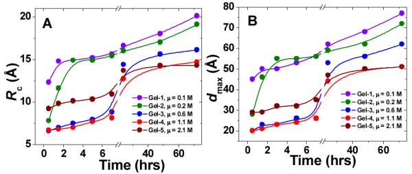
Time-evolution of the cross-sectional parameters of the hydrogel fibers formed at different ionic strengths: (A) radius of gyration of the cross-section, R_c; (B) maximum cross-section dimension, d_max. The lines represent a basic B-spline fit of the data. Violet: Gel-1; green: Gel-2; blue: Gel-3; red: Gel-4; brown: Gel-5.

As seen from Figure 5, the trend in the growth of both cross-sectional parameters (R_c and d_max) over time also follows the order Gel-1 > Gel-2 > Gel-5 > Gel-3 > Gel-4 which was observed from the rheological (Figure 2(A)) and I(0) (Figure 4(E)) data. On the other hand, at the time of gelation completion (72 hrs), the values of the radii of gyration of the cross-section, R_c, and maximum cross-sectional dimensions, d_max, consistently decrease with ionic strength increase (Figure 5, Gel-1 > Gel-2 > Gel-3 > Gel-4 > Gel-5). Such contraction of the fiber’s cross-sectional dimensions with increasing ionic strength is also pictorially demonstrated by the changes in the 2D shapes of fiber cross-section over gelation time (Figure 6, top panel). This overall dimensional compaction of the cross-section with ionic strength growth is also evident from the narrowing of the pair-wise distance distribution functions of the cross-section pair distribution function P_c(r) (Figure 6, bottom panel). In Figure 6 (bottom panel), at higher ionic strength P_c(r) comes to 0 at ~50 Å, illustrating the shrinking of the cross-sectional d_max by more than 25 Å (cf. with d_max ~ 77 Å at the lowest ionic strength, 0.1 M). Note that the observed shrinking of the fiber cross-section is consistent with the above mentioned possibility of the fiber compaction due to significant drop in the Debye screening length at higher ionic strength. Moreover, the formation of less compact, more tenuous fibers with bigger cross-section at lower ionic strength results in more turbid hydrogels as compared to those assembled at higher ionic strength (Figure 1).

Fig. 6.

SAXS monitoring of the ionic strength effects on the gelation process. Top panel shows the time evolution of the 2D average cross-section of the peptide fibers. Bottom panel show the changes in the corresponding pair-wise distance distribution function of the cross-section, P_c(r). Violet: Gel-1; green: Gel-2; blue: Gel-3; red: Gel-4; wine: Gel-5. P_c(r) functions in each case were normalized by their maximum zero-angle scattering intensity of cross-section, I_c(0).

It also stands to mention that as seen from the top panel of Figure 6, at lower ionic strength, the increase in the cross-sectional dimensions, d_max, is rather fast as opposed to the higher ionic strength case, where the changes in d_max within first 7 hours of gelation appear to be insignificant. One might possibly suggest that at lower ionic strength, the cross-sectional and longitudinal assemblies of the fibers are almost simultaneous, while at higher ionic strength, the longitudinal growth of the fiber to a certain extent outpaces the cross-sectional growth. However, this suggestion still needs to be verified based on the data of fiber length which, unfortunately, are beyond the limits of the maximum resolved size of our SAXS setup.

Interestingly, the same Gel-1 > Gel-2 > Gel-5 > Gel-3 > Gel-4 growth order appears to be characteristic not only to linear dimensions of the fibers cross-section (R_c, d_max) but also to the fibers cross-sectional area S_c (Figure 7(A)). However, as opposed to consistent drop in R_c, d_max with increasing μ at the end of gelation after 72 hours (Figure 5 and Figure 6), the final values of S_c also stand in the same Gel-1 > Gel-2 > Gel-5 > Gel-3 > Gel-4 order (Figure 7A).

Fig. 7.

(A). Growth of peptide fiber cross-section area, S_c, at different ionic strengths. The lines represent a basic B-spline fit of the data. Violet: Gel-1, green: Gel-2, blue: Gel-3, red: Gel-4, wine: Gel-5. (B). Dependence of peptide fiber cross-section area, S_c (z-axis)_, on time and ionic strength (x- and y-axis). 3D plot is made using Origin 8.1 (OriginLab) software, wireframe created using thin plate spline (TPS) algorithm.

Possible explanation of the observed effects of ionic strength could be based on the consideration of the interplay between electrostatic and hydrophobic interactions which control the assembly of the oppositely charged individual peptide modules into the fibrous hydrogel network. At low ionic strength, the electrostatic attraction between negative E11 and positive K11 will define the assembly, and the peptides aggregate quickly and form thicker fibers. When the ionic strength goes up, the peptides aggregation will be slower and the fibers will be thinner. At much higher ionic strength (our highest value of 2.1 M for Gel-5), electrostatic attractions become even less relevant whereas hydrophobic interactions become strong enough to control the fiber formation. Such qualitative explanation is consistent with the dependence of the fiber cross-sectional area S_c on gelation time and ionic strength, as represented by the 3D surface shown in Figure 7 (B).

Here, the evident trough in S_c in the μ range from 0.7 M to 1.4 M could be attributed to the situation where electrostatic attractions become mostly shielded, while hydrophobic interactions are still not strong enough to control the assembly—this slows down the gelation and defines the formation of thinner fibers. Whereas with the increase of ionic strength up to 2.1 M, hydrophobic interactions become strong enough to accelerate the assembly and produce somewhat thicker fibers (Figure 7B).

One would expect that larger fiber cross-sections of the fiber translate into higher elastic modulus G’ (Figure 2A). However, while the radius of gyration of fiber cross-section follows the order, Gel-1 > Gel-2 > Gel-3 > Gel-4 > Gel-5, the plateau elastic modulus follows the opposite order Gel-5 > Gel-4 > Gel-3 > Gel-2 > Gel-1. This result suggests that structural features other than the dimensional parameters of individual fiber cross-sections also contribute to the elastic modulus of hydrogels. One such structural feature is the arrangement of individual fibers, which is represented by the cross-sectional correlation length L_c. L_c reflects the average “mesh size” between fibers in the section plane of the fiber network. As seen from Figure 8, lnL_c decreases linearly with lnμ. This implies that the network density increases with the ionic strength. Another structural feature is the persistence length of individual fibers, L_p, which describes their rigidity. As seen from Figure 8, lnL_p increases linearly with the ionic strength. Therefore, hydrogels of higher ionic strength comprise of thinner (smaller R_c and d_max) but more rigid fibers (larger L_p) of higher fiber network density (smaller L_c).

Fig. 8.

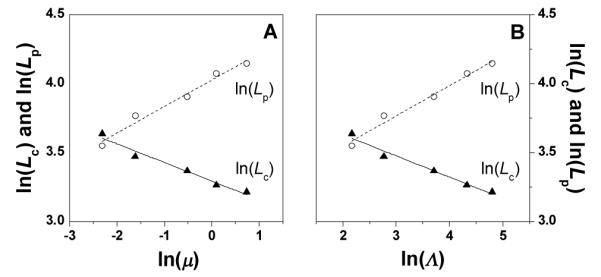
ln(L_c) and ln(L_p) vs. ln(μ) (A) and ln(Λ) (B), the solid and dash line is the linear fitting results. In panel A, the adjusted R² of ln(L_c) vs. ln(μ) is 0.962, the intercept is 3.291, and the slope is −0.135; the adjusted R² of ln(L_p) vs. ln(μ) is 0.970, the intercept is 4.024, and the slope is 0.192. In panel B, the adjusted R² of ln(L_c) vs. ln(Λ) is 0.965, intercept is 3.937, and the slope is −0.154; the adjusted R² of ln(L_p) vs. ln(Λ) is 0.975, the intercept is 3.105, and the slope is 0.220.

In terms of structural properties, lnL_c and lnL_p display linear dependency on lnμ (Figure 8A). In terms of mechanical properties, G’ displays a linear dependency on lnμ (Figure 3A). Thus one would expect certain correlation between G’ and lnL_c or lnL_p. It has been previously shown that ionic strength increase in protein hydrogels leads to noticeable decrease in correlation length L_c.⁴⁵ Figure 9A plots lnL_c and lnL_p vs. G’ and Figure 9B plots lnL_c and lnL_p vs. lnG’. Indeed G’ decrease with L_c but increases with L_p.

Fig. 9.

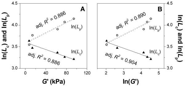
ln(L_c) and ln(L_p) vs. G’ (A); ln(L_c) and ln(L_p) vs. ln(G’) (B).

The MacKintosh theory⁴⁶ sheds light on the correlation between G’ on the one hand and L_c and L_p on the other. According to this theory, G’, L_c and L_p in a polymer hydrogel satisfy the following relationship:

$$G^{\prime }~\frac{L_p^n}{L_c^{m}kT}$$ (6)

Eqn. (6) suggests that G’ decreases with L_c but increases with L_p, as seen in Figure 9. However, the MacKintosh theory implies a linear correlation between lnG’ and lnL_c and lnL_p. In our case, both lnG’ and G’ have good but not perfect linear correlation with lnL_c and lnL_p (Figure 9). This indicates that although L_c and L_p make significant contribution to G’, there are other contributing factors. In other words, the MacKintosh theory captures the main but not all aspects of this class of hydrogels. Possibly, at lower ionic strength, where L_p < L_c, the MacKintosh theory which is valid for semiflexible chains with L_c ≤ L_p,⁴⁶ reduces to the case of flexible chains where⁴⁷

$$G^{\prime }~\frac{kT}{L_c^3}$$ (7)

Thus, the formation of more flexible fibers, more heterogeneous hydrogels at lower ionic strength could explain the deviation from the MacKintosh theory and the loss of expected linear correlation between G’ and lnL_c (or lnL_p) in Figure 9A.

In summary, it has been shown that higher ionic strength slows down the hydrogelation process significantly because electrostatic attractions between the two oppositely charged gelators are screened. On the other hand, higher ionic strength enhances the hydrophobic interactions between the peptide gelators, leading to higher elastic modulus. Apparently, electrostatic attraction plays a more dominant role in gelation kinetics while hydrophobic interaction plays a more dominant role in hydrogel stiffness.

Transport properties

Using the pulse-field gradient NMR technique, the self-diffusion coefficients of water (solvent) and tfF (solute), D_water and D_tfF, in hydrogels and in solutions were measured. D_water and D_tfF both decrease linearly with the ionic strength in hydrogels and in solutions (Figure 10). The slope of this linear dependency in hydrogels is ca. 10% larger in the hydrogel than in the solution. This result indicates that ionic strength-induced decrease of the self-diffusion coefficient is mainly caused by the interaction of water and tfF with NaCl, with variations of hydrogel stiffness and structure playing only a minor role. This is hardly surprising considering that the hydrogels contain only 2 wt% of peptides and that both water and tfF molecules are much smaller than the mesh size of the hydrogels, which is ca. 30 Å (see L_c values in Figure 8). Thus, this type of hydrogels allows essentially free diffusion of small molecules inside its fiber network.

Fig. 10.

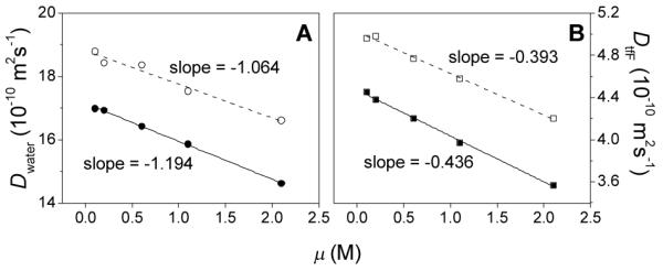
(A) Diffusion coefficients of H₂O (D_water) in solutions and hydrogels of various ionic strengths. Hollow circles: D_water in solutions; solid circles: D_water in hydrogels. Dash and solid lines are the linear fitting results. The goodness of fitting (adjusted R²) is 0.964 and 0.999, respectively. (B) Diffusion coefficients of tfF (D_tfF) in solutions and hydrogels of various ionic strengths. Hollow squares: D_tfF in solutions; solid squares: D_tfF in hydrogels. Dash and solid lines are the linear fitting results. The goodness of fitting (adjusted R²) is 0.993 and 0.997, respectively.

Conclusion

In our peptide hydrogel system, the elastic modulus G| increases linearly with the logarithm of the ionic strength while the gelation process slows down as the ionic strength increases. However, there is a rebound of gelation speed when the ionic strength is above 2M. SAXS analysis indicates the higher ionic strength leads to thinner but more rigid peptides that are more closely packed. The self-diffusion coefficient of small molecules inside the hydrogels decreases linearly with the ionic strength, but such decrease is predominantly a salt effect rather than barriers imposed by the hydrogel matrix.

references

- 1.Kopecek J. Biomaterials. 2007;28:5185. doi: 10.1016/j.biomaterials.2007.07.044. [DOI] [PMC free article] [PubMed] [Google Scholar]
- 2.Zhang S, Gelain F, Zhao X. Seminars in Cancer Biology. 2005;15:413. doi: 10.1016/j.semcancer.2005.05.007. [DOI] [PubMed] [Google Scholar]
- 3.Lee KY, Mooney DJ. Chem. Rev. 2001;101:1869. doi: 10.1021/cr000108x. [DOI] [PubMed] [Google Scholar]
- 4.Zhou M, Smith AM, Das AK, Hodson NW, Collins RF, Ulijn RV, Gough JE. Biomaterials. 2009;30:2523. doi: 10.1016/j.biomaterials.2009.01.010. [DOI] [PubMed] [Google Scholar]
- 5.Peppas NA, Hilt JZ, Khademhosseini A, Langer R. Adv. Mater. 2006;18:1345. [Google Scholar]
- 6.Yan C, Pochan DJ. Chem. Soc. Rev. 2010;39:3528. doi: 10.1039/b919449p. [DOI] [PMC free article] [PubMed] [Google Scholar]
- 7.Engler AJ, Sen S, Sweeney HL, Discher DE. Cell. 2006;126:677. doi: 10.1016/j.cell.2006.06.044. [DOI] [PubMed] [Google Scholar]
- 8.Saha K, Keung AJ, Irwin EF, Li Y, Little L, Schaffer DV, Healy KE. Biophys. J. 2008;95:4426. doi: 10.1529/biophysj.108.132217. [DOI] [PMC free article] [PubMed] [Google Scholar]
- 9.Ramachandran S, Flynn P, Tseng Y, Yu YB. Chem. Mater. 2005;17:6583. [Google Scholar]
- 10.Haines-Butterick L, Rajagopal K, Branco M, Salick D, Rughani R, Pilarz M, Lamm M. s., Pochan DJ, Schneider JP. Proc. Natl. Acad. Sci. U. S. A. 2007;104:7791. doi: 10.1073/pnas.0701980104. [DOI] [PMC free article] [PubMed] [Google Scholar]
- 11.Feng Y, Lee M, Taraban M, Yu YB. Chem. Comm. 2011;47:10455. doi: 10.1039/c1cc13943f. [DOI] [PMC free article] [PubMed] [Google Scholar]
- 12.Koutsopoulos S, Unsworth LD, Nagai Y, Zhang S. Proc. Natl. Acad. Sci. U. S. A. 2009;106:4623. doi: 10.1073/pnas.0807506106. [DOI] [PMC free article] [PubMed] [Google Scholar]
- 13.Branco MC, Pochan DJ, Wagner NJ, Schneider JP. Biomaterials. 2009;30:1339. doi: 10.1016/j.biomaterials.2008.11.019. [DOI] [PMC free article] [PubMed] [Google Scholar]
- 14.Branco MC, Pochan DJ, Wagner NJ, Schneider JP. Biomaterials. 2010;31:9527. doi: 10.1016/j.biomaterials.2010.08.047. [DOI] [PMC free article] [PubMed] [Google Scholar]
- 15.Zhang S, Holms T, Lockshin C, Rich A. Proc. Natl. Acad. Sci. U. S. A. 1993;90:3334. doi: 10.1073/pnas.90.8.3334. [DOI] [PMC free article] [PubMed] [Google Scholar]
- 16.Ozbas B, Kretsinger J, Rajagopal K, Schneider JP, Pochan DJ. Macromolecules. 2004;37:7331. [Google Scholar]
- 17.Van Tomme SR, De Geest BG, Braeckmans K, De Smedt SC, Siepmann F, Siepmann J, van Nostrum CF, Hennink WE. J. Control. Release. 2005;110:67. doi: 10.1016/j.jconrel.2005.09.005. [DOI] [PubMed] [Google Scholar]
- 18.Skouri R, Schosseler F, Munch JP, Candau SJ. Macromolecules. 1995;28:197. [Google Scholar]
- 19.Schexnailder P, Loizou E, Porcar L, Butler P, Schmidt G. Phys. Chem. Chem. Phys. 2009;11:2760. doi: 10.1039/b820452g. [DOI] [PubMed] [Google Scholar]
- 20.Johnson TD, Lin SY, Christman KL. Nanotechnology. 2011;22:494015. doi: 10.1088/0957-4484/22/49/494015. [DOI] [PMC free article] [PubMed] [Google Scholar]
- 21.Jin M, Grodzinsky AJ. Marcromolecules. 2001;34:8330. [Google Scholar]
- 22.Feng Y, Taraban M, Yu YB. Soft Matter. 2011;7:9890. doi: 10.1039/C1SM06389H. [DOI] [PMC free article] [PubMed] [Google Scholar]
- 23.Ulijn RV, Smith AM. Chem. Soc. Rev. 2008;37:664. doi: 10.1039/b609047h. [DOI] [PubMed] [Google Scholar]
- 24.Gill SC, Von Hippel PH. Anal. Biochem. 1989;182:319. doi: 10.1016/0003-2697(89)90602-7. [DOI] [PubMed] [Google Scholar]
- 25.Chan WC, White PD. Fmoc Solid Phase Peptide Synthesis: A Practical Approach. Oxford University Press; New York: 2000. [Google Scholar]
- 26.Caplan MR, Schwartzfarb EM, Zhang S, Kamm RD, Lauffenburger DA. Biomaterials. 2002;23:219. doi: 10.1016/s0142-9612(01)00099-0. [DOI] [PubMed] [Google Scholar]
- 27.Hyland LL, Taraban MB, Feng Y, Hammouda B, Yu YB. Biopolymers. 2012;97:177. doi: 10.1002/bip.21722. [DOI] [PMC free article] [PubMed] [Google Scholar]
- 28.Whitten A, Trewhella J. Micro and Nano Technologies in Bioanalysis. Humana; New York: 2009. Small-Angle Scattering and Neutron Contrast Variation. [Google Scholar]
- 29.Kline SR. J. Appl. Cryst. 2006;39:895. [Google Scholar]
- 30.Pedersen JS, Shurtenberger P. Macromolecules. 1996;29:7602. [Google Scholar]
- 31.Chen W-R, Buter PD, Magid LJ. Langmuir. 2006;22:6539. doi: 10.1021/la0530440. [DOI] [PubMed] [Google Scholar]
- 32.Svergun DI. J. Appl. Cryst. 1992;25:495. [Google Scholar]
- 33.Konarev PV, Volkov VV, Sokolova AV, Koch MHJ, Svergun DI. J. Appl. Cryst. 2003;36:1277. [Google Scholar]
- 34.Glatter O, Kratky O, editors. Small Angle X-Ray Scattering. Academic Press; London: 1982. [Google Scholar]
- 35.Svergun DI. Biophys. J. 1999;76:2879. doi: 10.1016/S0006-3495(99)77443-6. [DOI] [PMC free article] [PubMed] [Google Scholar]
- 36.Whitten AE, Jeffries CM, Harris SP, Trewhella J. J. Proc. Natl. Acad. Sci. U. S. A. 2008;105:18360. doi: 10.1073/pnas.0808903105. [DOI] [PMC free article] [PubMed] [Google Scholar]
- 37.Ilavsky J, Jemian P. J. Appl. Crystallogr. 2009;42:347. doi: 10.1107/S160057671800643X. [DOI] [PMC free article] [PubMed] [Google Scholar]
- 38.Debye P, Bueche AM. J. Appl. Phys. 1949;20:518. [Google Scholar]
- 39.Soni VK, Stein RS. Macromolecules. 1990;23:5257. [Google Scholar]
- 40.Wu DH, Chen AD, Johnson CS. J. Magn. Reson., A. 1995;115:260. [Google Scholar]
- 41.Russel WB, Saville DA, Schowalter WR. Colloidal Dispersions. Cambridge University Press; 1989. [Google Scholar]
- 42.Yoshioka H, Mikami M, Mori Y, Tsuchida E. J. Macromol. Sci. A: Pure Appl. Chem. 1994;31:121. [Google Scholar]
- 43.Joshi SC. Materials. 2011;4:1861. doi: 10.3390/ma4101861. [DOI] [PMC free article] [PubMed] [Google Scholar]
- 44.Guinier A. Ann. Phys. (Paris) 1939;12:161. [Google Scholar]
- 45.Chatterjee S, Bohidar HB. Int. J. Biol. Macromol. 2005;35:81. doi: 10.1016/j.ijbiomac.2005.01.002. [DOI] [PubMed] [Google Scholar]
- 46.MacKintosh FC, Käs J, Janmey PA. Phys. Rev. Lett. 1995;75:4425. doi: 10.1103/PhysRevLett.75.4425. [DOI] [PubMed] [Google Scholar]
- 47.de Gennes PG. Scaling Concepts in Polymer Physics. Cornell University Press; Ithaca, & London: 1979. [Google Scholar]
Associated Data
This section collects any data citations, data availability statements, or supplementary materials included in this article.