R*₂ Mapping in the Presence of Macroscopic B₀ Field Variations

Abstract

R*₂ mapping has important applications in MRI, including functional imaging, tracking of super-paramagnetic particles, and measurement of tissue iron levels. However, R*₂ measurements can be confounded by several effects, particularly the presence of fat and macroscopic B₀ field variations. Fat introduces additional modulations in the signal. Macroscopic field variations introduce additional dephasing that results in accelerated signal decay. These effects produce systematic errors in the resulting R*₂ maps and make the estimated R*₂ values dependent on the acquisition parameters. In this study, we develop a complex-reconstruction, confounder-corrected R*₂ mapping technique, which addresses the presence of fat and macroscopic field variations for both 2D and 3D acquisitions. This technique extends previous chemical shift-encoded methods for R*₂, fat and water mapping by measuring and correcting for the effect of macroscopic field variations in the acquired signal. The proposed method is tested on several 2D and 3D phantom and in vivo liver, cardiac, and brain datasets.

Mapping of R*₂ relaxivity (R*₂ = 1/T*₂) has multiple important applications in MRI, including blood oxygenation level dependent functional imaging (1–3), detection and tracking of super-paramagnetic iron oxides (4), and assessment of iron content in brain (5), heart (6,7), and liver (8,9). R*₂ maps can be obtained from rapid acquisitions, such as spoiled gradient-echo multiecho sequences, which makes this technique particularly attractive for body imaging applications where motion is an important challenge (8).

However, R*₂ mapping is affected by several confounding factors, particularly fat and macroscopic B₀ field variations. In this study, R*₂ refers to the intrinsic relaxation properties of a tissue or sample (at a given field strength), independent of external B₀ field variations and fat content. The presence of fat introduces additional modulations in the acquired signal (10–12) and can lead to severe bias in R*₂ measurements. The presence of macroscopic B₀ field variations introduces additional intravoxel dephasing in the acquired signal and results in faster signal decay, which can lead to severe overestimation of R*₂ (13), particularly in regions with sharp susceptibility changes (e.g., near tissue/air interfaces). These confounders generally make R*₂ maps highly dependent on the acquisition parameters. For instance, in the presence of fat the apparent R*₂ maps (without accounting for fat) will depend on the echo time (TE) combination. In the presence of macroscopic field variations, the apparent R*₂ maps will depend heavily on the spatial resolution (particularly, the slice thickness).

The presence of fat is often addressed by acquiring “in-phase echoes,” where the TEs are carefully selected, so that the signal from the water peak and the main methylene peak are in-phase. This approach largely removes the effects of fat but has several inherent limitations: (a) not all fat peaks are in-phase with water (just the main methylene peak) and (b) it requires relatively large echo spacings and first TE, which may not be optimal for measuring large R*₂ values (e.g., in the presence of iron). Alternative techniques such as chemical shift-based fat suppression (or use of spatial-spectral pulses) are sensitive to B₀ field inhomogeneities that can be significant in many applications, such as liver and heart imaging (11,14–17). Other techniques, such as short-tau inversion recovery fat nulling (18), are effective and can be made insensitive to B₀ and B₁ inhomogeneities but require the introduction of additional inversion pulses and result in a significant signal-to-noise ratio loss (11,16,17). Finally, chemical shift based techniques that perform fat–water separation and R*₂ estimation simultaneously (19,20) have the potential to overcome these limitations, and they can provide fat-corrected R*₂ measurements with good signal-to-noise ratio and using a wide variety of TE combinations.

Methods for correcting macroscopic field variations typically focus on the through-slice field variation and often (but not always) assume locally linear variations. These methods can be classified into two general categories: (a) methods that modify the acquisition to minimize field variation effects in the data (5,21–29) and (b) methods that correct the data by postprocessing (4,13,30–32). The first group of methods typically use several images obtained with higher resolution (or with different refocusing mis-adjustments) along the largest (slice) direction, which are subsequently magnitude-combined to prevent dephasing for increasing TEs (5,21,24,26,33). The second group of methods are based on modeling and correction for the effects of macroscopic field variations by postprocessing. Some of these methods require an additional, higher-resolution field-mapping acquisition (30,32), whereas others use a single acquisition to model and correct for field variations (13). Most methods are based on 2D multislice acquisitions and model the field variation as locally linear (4,13) or quadratic (32) through the slice. However, these methods do not address the presence of fat, which can be very abundant in certain organs (e.g., liver and pancreas), and typically they have been developed for 2D acquisitions under the assumption of ideal (boxcar) slice profiles (34). In practice, slice profiles often differ significantly from the ideal boxcar function, which can have a dramatic effect on the signal dephasing and decay introduced by macroscopic field variations.

In this study, we have developed a method for R*₂ mapping in the presence of fat and macroscopic field variations, for both 2D and 3D acquisitions (34), and accounting for the effects of nonideal slice profiles (2D) and k-space windowing (3D). The proposed method is based on a chemical shift-encoded acquisition with short echo spacings, to allow fat–water separation in addition to R*₂ mapping. Because this acquisition also can be used to obtain a B₀ field map, we measure the B₀ field and correct for the effects of macroscopic field variations to obtain R*₂ maps that are independent of the acquisition parameters. The following sections include the mathematical derivation of the proposed method for 2D and 3D acquisitions, a description of the experimental methods, phantom and in vivo results, and a discussion of the properties and limitations of the method.

THEORY

Characterizing the Effects of B₀ Variations

The signal obtained in a multiecho spoiled gradient-echo acquisition with TE “t” at location r₀, in the presence of fat and water as well as macroscopic B₀ field variation, can be modeled as:

$$s(t;r_0)={\int }_{{\mathbb{R}}^3}({\rho }_{\mathrm{W}}\left(\mathbf{r}\right)+{\rho }_{\mathrm{F}}\left(\mathbf{r}\right)c_{\mathrm{F}}\left(t\right)){\mathrm{e}}^{-R_2^{\ast }\left(\mathbf{r}\right)t}{\mathrm{e}}^{j2\pi -\gamma \Delta B_0\left(\mathbf{r}\right)t}\times \text{SRF}(\mathbf{r}-r_0)\mathrm{d}\mathbf{r}$$ [1]

where ρ_W(r) and ρ_F(r) are the water and fat amplitudes, respectively, $c_{\mathrm{F}}\left(t\right)={\sum }_{m=1}^M{\alpha }_m{\mathrm{e}}^{j2\pi f_{\mathrm{F},m}t}$ is the fat signal model, consisting of multiple spectral peaks with relative amplitudes α_m (normalized such that ${\sum }_{m=1}^M{\alpha }_m=1$), and frequencies f_F,m (19,35–37), R*₂(r) is the spatial distribution of R*₂ = 1/T*₂ (assumed common for water and fat, i.e., a “single-R*₂” model; Refs. 19,20,38, and 39), $-\gamma \Delta B_0\left(\mathbf{r}\right)$ is the magnetic field offset (in Hz), and SRF(r – r₀) is the spatial response function (SRF) of a voxel centered at r₀.

The SRF is, analogously to the point-spread function, a weighting function describing the influence of each spatial location on the current voxel. For example, in a 2D acquisition with ideal slice selection, the SRF along the slice direction is a boxcar function. Along Fourier-encoded directions in Cartesian acquisitions (in-plane directions for 2D acquisitions; all three directions for 3D acquisitions), the SRF is a sinc-like function (40,41). Parallel imaging effects on the SRF are not considered in this study (41).

If the magnetic field ΔB₀(r) varies slowly relative to the imaging resolution, it can be considered approximately constant over each voxel and the signal model in Eq. 1 can be reduced to the usual fat–water imaging signal model (including R*₂ and spectral modeling of fat). If ΔB₀(r) varies extremely rapidly, or the readout bandwidth is very low, the images will contain significant distortions. Note that the signal model in Eq. 1 does not include these distortions (it assumes that the slice-select and readout bandwidths are high enough that these effects can be neglected). For instance, in this study, the fat chemical shift artifact (for the main fat peak) typically results in a displacement of <1/3 voxel along the readout dimension.

Frequently in MR acquisitions, the spatial resolution is significantly coarser along one dimension (through-slice), compared with the remaining two dimensions (in-plane). In this case, the signal model in Eq. 1 can be simplified as:

$$s(t;z_0)={\int }_{\mathbb{R}}({\rho }_{\mathrm{W}}\left(z\right)+{\rho }_{\mathrm{F}}\left(z\right)c_{\mathrm{F}}\left(t\right)){\mathrm{e}}^{-R_2^{\ast }\left(z\right)t}{\mathrm{e}}^{j2\pi -\gamma \Delta B_0\left(z\right)t}\times \text{SRF}(z-z_0)\mathrm{d}z$$ [2]

where the spatial dependence of all parameters has been removed for the in-plane dimensions. The signal modulation effects introduced by background field gradients, and characterized by the SRF, depend on the type of acquisition (2D or 3D). These effects will be analyzed next.

2D Multislice Acquisitions

For 2D acquisitions with linear through-slice field variation ΔB₀(z) = ΔB₀(z₀) + G[z − z₀] and given slice profile SRF(z), we can assume ρ_W(z), ρ_F(z) and R*₂(z) to be constant through the slice. Then, Eq. 2 becomes:

$$s(t;z_0)=({\rho }_{\mathrm{W}}+{\rho }_{\mathrm{F}}{c}_{\mathrm{F}}\left(t\right)){\mathrm{e}}^{-R_2^{\ast }t}{\mathrm{e}}^{j2\pi -\gamma \Delta B_0\left(z_0\right)t}\times {\int }_{\mathbb{R}}{e}^{j2\pi -\gamma G[z-z_0]t}\text{SRF}(z-z_0)\mathrm{d}z,$$ [3]

where z₀ is the center of the slice and the integral can be evaluated over the support of the SRF (the locations where the SRF is nonzero). Therefore, the signal in Eq. 3 is modeled as the standard R*₂-corrected fat–water signal model (19), modulated by the term ${\int }_{\mathbb{R}}{\mathrm{e}}^{j2\pi -\gamma [z-z_0]Gt}\text{SRF}(z-z_0)\mathrm{dz}$, which accounts for accelerated signal decay due to macroscopic field variation. This integral term can easily be calculated numerically, for a given SRF and field gradient G along the z direction. In the case of an ideal slice profile (SRF is a boxcar function), Eq. 3 becomes (13):

$$s(t;z_0)=({\rho }_{\mathrm{W}}+{\rho }_{\mathrm{F}}{c}_{\mathrm{F}}\left(t\right)){\mathrm{e}}^{j2\pi -\gamma \Delta B_0\left(z_0\right)t}{\mathrm{e}}^{-R_2^{\ast }t}\times {\int }_{z_0-\Delta z∕2}^{z_0+\Delta z∕2}{\mathrm{e}}^{j2\pi -\gamma G[z-z_0]t}\mathrm{d}z$$ [4]

$$=({\rho }_{\mathrm{W}}+{\rho }_{\mathrm{F}}{c}_{\mathrm{F}}\left(t\right)){\mathrm{e}}^{j2\pi -\gamma \Delta B_0\left(z_0\right)t}{\mathrm{e}}^{-R_2^{\ast }t}\Delta z\text{sinc}(-\gamma G\Delta zt).$$ [5]

In the ideal slice profile case, the fat–water signal model is modulated by the term $\text{sinc}(-\gamma G\Delta zt)$, which will decay faster for larger field gradients or thicker slices (see Fig. 1, first row).

FIG. 1.

Signal modulation in 2D and 3D acquisitions with 10 mm resolution in the slice direction, in the presence of a linearly varying B₀ field. (Left) The true signal amplitude is a broad boxcar (resembling a large homogeneous object). The spatial response function is shown for five different imaging scenarios: 2D with ideal slice profile, 2D with nonideal profile, 3D (no k-space windowing, and slice away from object edge), 3D (no k-space windowing and slice near object edge), and 3D (with k-space windowing). (Right) Corresponding signal modulation for several different values of the B₀ gradient (from 0 to 4 Hz mm⁻¹). Macroscopic field variations introduce additional signal modulations, which are heavily dependent on the details of the acquisition (e.g., 2D vs. 3D, slice profile) and reconstruction (e.g., k-space windowing).

In practice, it is very difficult to obtain slice profiles close to the ideal boxcar profile, because of the long radio-frequency pulses that would be required. Nonideal slice profiles will not result in a sinc modulation of the acquired signal. In general, there will not be a closed-form expression for the modulation term, but it can be calculated easily by numerical integration (see Eq. 3), given a particular slice profile (obtained by calibration or by Bloch simulation). Figure 1 (second row) shows an example of the signal modulation in 2D imaging with an example nonideal slice profile. Figure 1 (top two rows) shows the different signal behavior in the presence of macroscopic field variations, as a function of the slice profile. This clearly demonstrates the need for accounting for accurate slice profiles for corrected R*₂ measurements. This effect will be analyzed experimentally using phantom data.

3D Acquisitions

In 3D imaging, the “slice” (z) dimension is also often acquired with coarser spatial resolution compared to the in-plane dimensions. For instance, this is usually needed in 3D liver acquisitions (42), to provide whole-liver coverage with fat–water separation and R*₂ mapping in a single breath-hold. For 3D acquisitions, the SRF is a sinc-like function with broad spatial support (as opposed to the narrower SRF in 2D experiments). For this reason, we model the parameters ρ_W and ρ_F as piecewise linear over several lobes of the SRF, while maintaining the fat fraction constant (i.e., overall signal amplitude a(z) = ρ_W(z) + ρ_F(z) piecewise linear over the SRF), R*₂ constant, and field inhomogeneity ΔB₀(z) locally modeled as a low-order polynomial. With these approximations, Eq. 2 can be expressed as follows:

$$s(t;z_0)=({\rho }_{\mathrm{W}}+{\rho }_{\mathrm{F}}{c}_{\mathrm{F}}\left(t\right)){\mathrm{e}}^{-R_2^{\ast }t}{\mathrm{e}}^{j2\pi -\gamma \Delta B_0\left(z_0\right)t}\times {\int }_{\mathbb{R}}a\left(z\right){\mathrm{e}}^{j2\pi -\gamma [\Delta B_0\left(z\right)-\Delta B_0\left(z_0\right)]t}\text{SRF}(z-z_0)\mathrm{d}z$$ [6]

i.e., the signal is modeled as the standard R*₂-corrected fat–water signal model (19), modulated by the term ${\int }_{\mathbb{R}}a\left(z\right){\mathrm{e}}^{j2\pi -\gamma [\Delta B_0\left(z\right)-\Delta B_0\left(z_0\right)]t}\text{SRF}(z-z_0)\mathrm{dz}$, analogously to the 2D case. In this study, a third-order polynomial is used to model field variations, and the modulation term is calculated numerically by integrating over several lobes of the SRF (see Fig. 1). The term a(z) is approximated by a piecewise linear function using the amplitude of the normalized signals (sum of fat and water, normalized to the signal at z₀) estimated from an initial fat–water separation (uncorrected for macroscopic field variations). The assumption of a constant fat fraction is made for simplicity and may be a limitation in regions of rapidly varying fat fraction.

For 3D acquisitions, the signal modulation due to B₀ variations is more complicated than in the 2D case because of the broad spatial support of the SRF (i.e., the SRF has lobes extending much farther away than typical 2D acquisitions with the same nominal resolution). This makes the modulation in 3D acquisitions dependent on the location of the slice. For instance, it is possible to have a voxel with significant field variation but without additional decay (because the modulation can be nearly flat until a given TE is reached). However, this is not the case for slices near the edge of an object, e.g., near the dome of the liver (see Fig. 1). This should be taken into account when performing R*₂ measurements.

Additionally, k-space filtering (windowing) is often applied in practice to remove Gibbs ringing and improve signal-to-noise ratio. These improvements come at the cost of a loss of spatial resolution and a change in the SRF (typically wider main lobe and reduced side lobes). Analogously to the 2D case, this change in SRF results in different signal behavior in the presence of background field gradients (see Fig. 1, bottom row). Fortunately, the effects of k-space windowing can be incorporated into the proposed method by including windowing into the SRF (by convolving the original 3D SRF with the appropriate image-domain filter corresponding to the k-space window used). The 3D data used in this study has been k-space windowed using a modified Tukey window (43).

In-Plane Field Variations

Macroscopic field variations along the in-plane directions can be accounted for similar to the “z” direction in 3D acquisitions, including the application of k-space windowing. However, in-plane spatial resolution is typically significantly higher than in through-slice directions. Thus, signal modulations due to in-plane field variations are typically much smaller than those along the “z” direction. For simplicity, this study focuses on field variations along the “z” direction.

Correcting for B₀ Field Variations

The proposed method can be summarized as follows (see Fig. 2):

1. Perform initial fat–water separation with R*₂ and B₀ field map estimation (19,44). Note that the R*₂ and B₀ maps calculated in this step will be corrected for the presence of fat (as fat is included in the signal model).

2. At each voxel, compute the field variation along the slice direction based on the B₀ field map, and estimate the signal modulation due to macroscopic field variations.

3. Given the signal modulation at each voxel, re-estimate the unknown parameters (ρ_W, ρ_F, ΔB₀, and R*₂) by least-squares data fitting using the corrected signal model (Eqs. 3 and 6 in 2D and 3D, respectively).

FIG. 2.

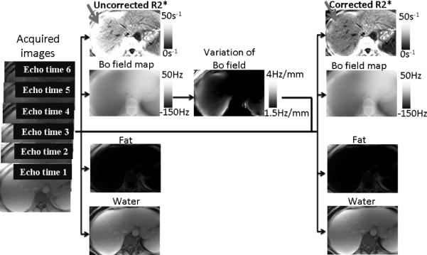
Schematic view of the proposed method.

Least-squares fitting can be performed using a modified Levenberg–Marquardt algorithm (“lsqnonlin” in Matlab). In this study, we include the modulation due to field variations in the signal model during parameter estimation (step 3), rather than “removing” this modulation from the data (dividing the acquired signal by the estimated modulation). In the presence of significant additional decay (i.e., if the modulation term approaches zero for later TEs), removing the modulation would result in significant noise amplification in the later echoes, which is avoided by simply including the modulation in the signal model and least-squares fitting the original data.

MATERIALS AND METHODS

Phantom Experiments

Phantom experiments were performed on a large cylindrical water phantom doped with CuSO₄, at 1.5T (Signa HDxt, GE Healthcare, Waukesha, WI) using a single-channel head coil. Phantom acquisitions were performed using investigational versions of a spoiled gradient-echo multiecho sequence with monopolar readout and flyback gradients, both in 2D (45) and in 3D (42). 3D acquisitions used a modified Tukey k-space window performed before Fourier transform in the slice direction (43).

Acquisition parameters for 2D imaging included: 16 echoes, TE_min = 1.8 ms, ΔTE = 2.5 ms, axial plane, readout direction R/L, matrix size 192 × 144, slice thickness 10 mm five slices, flip angle = 10°, pulse repetition time (TR) = 66 ms, BW = ±62.5 kHz.

Acquisition parameters for 3D imaging included: 16 echoes, TE_min = 1.5 ms, ΔTE = 2.6 ms, axial plane, readout direction R/L, matrix size 192×144, slice thickness 10 mm, 32 slices, flip angle = 10°, TR data = 60.6 ms, BW = ±62.5 kHz.

Phantom were obtained multiple times, in the presence of purposefully applied B₀ gradients along the slice direction. These were applied using the system's linear shim gradients, and were increased monotonically from 0 to ~ 4.5 Hz mm⁻¹, which covers the range of gradients we have observed in vivo in typical liver acquisitions.

Uncorrected R*₂ measurements from phantom data were performed twice, using all 16 and the first 6 echoes, respectively, to evaluate the dependence of uncorrected measurements on the acquisition parameters.

In Vivo Experiments

Subjects were scanned after obtaining informed written consent and with approval of the local Institutional Review Board. In vivo experiments were performed at 1.5 and 3.0T (GE Healthcare, Waukesha, WI), using an eight-channel phased array cardiac coil, eight-channel body phased array coil, or eight-channel head coil. In vivo imaging used the same multiecho spoiled gradient-echo sequences (2D and 3D) used in the phantom experiments. Multicoil data were combined prior to fat–water separation using the eigenvector filter method described by Walsh et al. (46).

Liver 2D imaging was performed at 1.5T with six echoes, TE_min = 1.44 ms, ΔTE = 1.84 ms (45). Other acquisition parameters included: axial plane, readout direction R/L, matrix size 256 × 128, slice thickness 6 and 10 mm, 11 slices, flip angle = 15°, TR = 22.5 ms, BW = ±125 kHz, scan time 24 s. Acquisitions were obtained with different slice thicknesses (6 and 10 mm) to evaluate the impact of slice thickness on uncorrected and corrected R*₂ measurements.

Liver 3D imaging was performed at 1.5 and 3.0T with six echoes, TE_min = 1.2 ms, ΔTE = 2.0 ms (1.5T), TE_min = 1.2 ms, ΔTE = 1.0 ms (3.0T using interleaved readout). Other acquisition parameters included: axial plane, readout direction R/L, matrix size 256 ± 128, slice thickness 10 mm, 24–28 slices, flip angle = 5°, TR 8–14 ms, BW = ±125 kHz, scan time 20 s.

Brain 3D data were acquired at 3.0 T with 12 echoes using two interleaved echo trains, with overall TE_min = 1.7 ms, ΔTE = 1.4 ms. Other acquisition parameters included: axial plane, readout direction A/P, matrix size 256 × 256, slice thickness 3 mm, 44 slices, flip angle 11°, TR = 20.6 ms, scan time 5 min 16 s. Brain data were using the same fat–water model for simplicity, although in practice a fat component is not needed in most brain tissues.

Cardiac 2D acquisitions were performed at 1.5 T with eight echoes, TE_min = 1.61 ms, ΔTE 1.86 ms, acquiring a single slice per breath-hold. Other acquisition parameters included: short-axis view, matrix size 192 × 192, slice thickness 8 mm, eight slices, flip angle 20°, TR = 18 ms, BW = ±100 kHz, scan time 21 s per slice.

RESULTS

Phantom

Phantom results from 2D and 3D acquisitions in the presence of varying field gradients are shown in Fig. 3. The R*₂ values in the absence of significant field gradients is 11 s⁻¹ for both acquisitions. For increasing field gradients, the standard (uncorrected) R*₂ measurements increase monotonically, up to nearly 120 s⁻¹ (2D) and 180 s⁻¹ (3D). For the 2D acquisition, Fig. 3 (top) also shows the corrected measurements under the assumption of ideal slice profiles. Note how these have smaller errors than the uncorrected measurements but still increase monotonically with increasing field gradients, up to nearly 50 s⁻¹ for the largest gradient. Finally, the corrected measurements accounting for the nonideal slice profile (calculated from the radiofrequency pulse by Bloch simulation) appear nearly flat for varying field gradients, with a maximum error no greater than 4 s⁻¹.

FIG. 3.

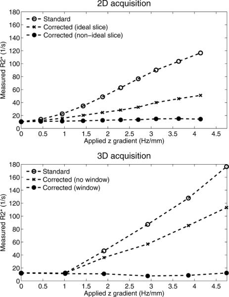
Phantom R*₂ measured in 2D and 3D acquisitions, in the presence of a linearly varying B₀ field. If uncorrected, macroscopic field variations lead to large errors in R*₂ estimation. Note the importance of accounting for the acquisition (slice profile in 2D experiments) and reconstruction parameters (k-space windowing along the z direction in 3D experiments).

Along with the uncorrected measurements, the 3D acquisition (Fig. 3, bottom) also shows the corrected measurements under the assumption of unfiltered k-space data. These still have large errors, with estimates reaching nearly 120 s⁻¹. The corrected measurements accounting for k-space windowing have much reduced variability in the presence of varying field gradients, with a maximum error of 4 s⁻¹.

Figure 4 shows the corresponding fat fraction measurement results for 2D and 3D acquisitions, comparing the uncorrected method using 16 and 6 echoes and the corrected method using 16 echoes. Fat fraction estimates are less affected by macroscopic field variations, compared to R*₂ estimates, but errors also appear for very rapid field variations. Note that these errors are dependent on the choice of acquisition parameters (e.g., TE combination).

FIG. 4.

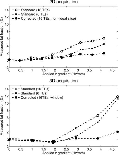
Fat fractions measured on a water-only phantom (fat fraction = 0%) in 2D and 3D acquisitions, in the presence of a linearly varying B₀ field. The results show the uncorrected measures using all 16 echoes, as well as using only the first six echoes, and the corrected measures using all 16 echoes. Fat fractions are less affected than R*₂ by macroscopic field variations. However, very large field gradients can still introduce errors in fat fraction measurement. Note the dependence of apparent fat fraction on the choice of TE combination, in the presence of very large field gradients.

In vivo

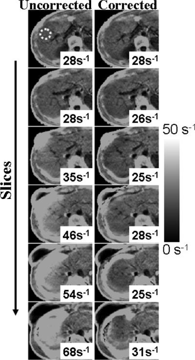
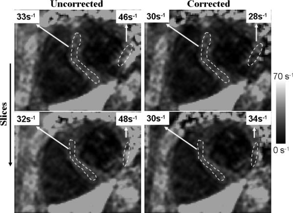
Figure 5 shows liver R*₂ measurements from a 2D multislice acquisition. As the slices approach the dome of the liver, field variations become more severe (due to susceptibility effects near the interface between the liver and the adjacent lung), and uncorrected R*₂ measurements appear artifactually high (20 s⁻¹ overestimation). Corrected R*₂ values (accounting for the nonideal slice profile) largely correct this overestimation.

FIG. 5.

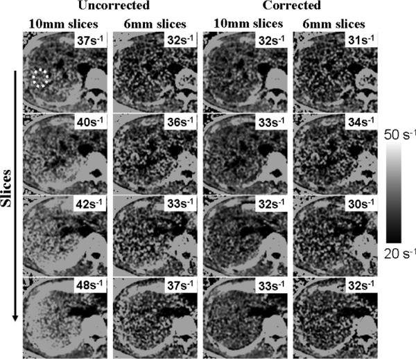
Liver R*₂ maps from a healthy volunteer, obtained using a 2D acquisition with 10-mm slices. (Left) Uncorrected. (Right) Corrected. Average R*₂ was measured from the area inside the yellow dots (the same region-of-interest was measured in all slices for both reconstructions). Note the increase in apparent (uncorrected) R*₂ values as slices approach the dome of the liver. Susceptibility-corrected R*₂ remains nearly constant throughout all slices.

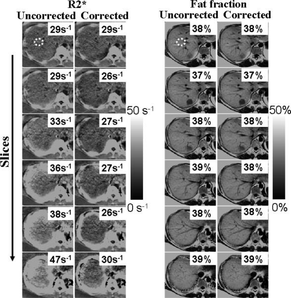
Figures 6 and 7 show liver R*₂ measurements from two different subjects using 3D acquisitions at 1.5 T. Figure 8 shows results from liver 3D acquisitions at 3.0 T. As the slices approach the dome of the liver, field variations become more severe, and uncorrected R*₂ measurements appear artifactually high (e.g., 40 s^–1 overestimation). Corrected R*₂ values (accounting for k-space windowing) largely correct this overestimation. Incomplete correction of R*₂ measurements appears near the edges of the liver for some slices approaching the dome of the liver. This is likely due to in-plane field variations (not corrected in this study), and/or significantly nonlinear spatial variation of the B₀ field at these locations.

FIG. 6.

Liver R*₂ maps from a healthy volunteer, obtained using a 3D acquisition with 10-mm slices. (Left) Uncorrected. (Right) Corrected. Note the increase in apparent (uncorrected) R*₂ values as slices approach the dome of the liver. Susceptibility-corrected R*₂ remains nearly constant throughout all slices.

FIG. 7.

Liver R*₂ and fat fraction maps from a patient with high liver fat, obtained using a 3D acquisition with 10 mm slices. R*₂ maps are affected by macroscopic field variations, which is largely corrected using the proposed technique. However, in this case, fat fraction measures appear almost constant even in the presence of field variations and require no correction.

FIG. 8.

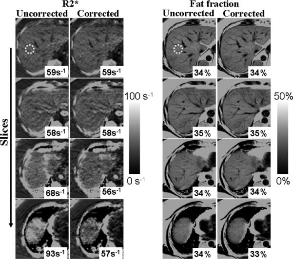
3 T results: liver R*₂ and fat fraction maps from a patient with high liver fat, obtained using a 3D acquisition with 8 mm slices. R*₂ maps are affected by macroscopic field variations, which is largely corrected using the proposed technique. Fat fraction measures are less sensitive to macroscopic field variations.

Figures 7 and 8 also show the corresponding fat fraction maps. Note that in these cases, the fat fraction remains nearly unperturbed in the presence of field variations and R*₂ errors, and both corrected and uncorrected methods produce similar estimates. For the relatively short TEs used in our liver acquisitions, the observed macroscopic field variations (typically < 3 Hz mm⁻¹) introduce an additional signal decay that can be accurately captured by an increased apparent R*₂ (thus introducing moderate fat quantification errors, as opposed to the phantom experiments with longer echo trains and more extreme field variations).

Figure 9 shows results from a 3D brain acquisition at 3.0 T, with 3 mm slices. Rapid field variations occur near the sinuses, which lead to errors in the apparent (uncorrected) R*₂ values. Corrected R*₂ values are in better agreement with literature values (13,47). In cardiac imaging (Fig. 10), rapid field variations appear, due to susceptibility variations near the heart/lung interface (48) or near large epicardial veins (49). Corrected R*₂ values show improved homogeneity.

FIG. 9.

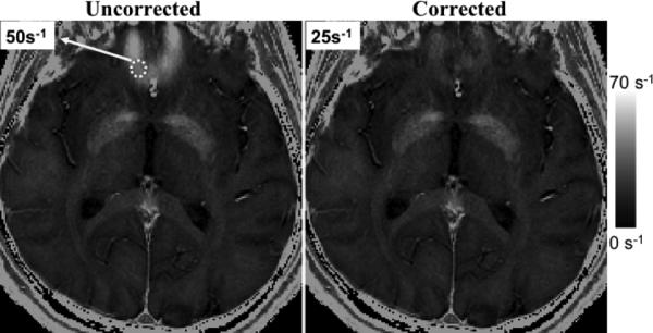
Brain R*₂ maps from 3D acquisition at 3 T. (Left) Uncorrected. (Right) Corrected.

FIG. 10.

Cardiac R*₂ maps from 2D acquisition at 1.5 T. (Left) Uncorrected. (Right) Corrected.

DISCUSSION

R*₂ quantification has many important applications in MRI, including blood oxygenation level dependent imaging, super-paramagnetic iron oxide tracking and iron quantification. However, its use is complicated by the presence of several confounders, specifically fat and macroscopic B₀ variations. These confounders introduce errors in R*₂ measurements and make the measurements dependent on acquisition parameters such as the TE combination and spatial resolution. For instance, in the context of liver R*₂ mapping for iron quantification, macroscopic field variations often lead to overestimations of 20–40 s⁻¹ in regions of severe susceptibility effects, which can result in R*₂ values clearly below the abnormal threshold (nearly 60 s⁻¹ for a 30-year-old subject at 1.5 T (8)) to appear as above the threshold. In this study, we have developed a confounder-corrected R*₂ mapping technique, by extending a previous fat-corrected method to also correct for the effects of B₀ variations.

In 2D acquisitions, confounder-corrected R*₂ mapping is feasible. Note that multislice acquisitions are needed to model and correct through-slice field variations. Additionally, confounder-corrected R*₂ mapping requires accounting for the slice profile, because the signal dephasing behavior, in the presence of field variations, depends heavily on the distribution of resonances present (not just on the nominal slice thickness). Arbitrary slice profiles do not lend themselves to a closed-form solution for the signal modulation in the presence of background field gradients, but this modulation can be easily calculated, given the slice profile, based on a simple numerical integration.

In 3D acquisitions, confounder-corrected R*₂ mapping is also feasible. An additional challenge in 3D acquisitions is the broad support of the SRF (sinc-like), which makes the modeling assumptions (e.g., locally smooth variation of the B₀ field) more stringent. In 3D imaging, it is also necessary to account for k-space filtering (windowing), which affects the SRF (typically broadening the main lobe and reducing the sidelobes). This is analogous to the need to account for nonideal slice profiles in 2D acquisitions. One question that has not been addressed in this study is whether k-space filtering prior to susceptibility-corrected R*₂ mapping is advantageous (due to the reduced influence of sidelobes, which complicate modeling of field variations).

Correction for background field variations is likely not necessary if the acquisition is performed with sufficiently high resolution relative to the field variations (33). For instance, for 2D six-echo acquisitions with TE_min 1.2 ms, ΔTE = 2.0 ms, in the presence of the B₀ gradients considered in Fig. 1 (maximum gradient 4 Hz mm⁻¹), acquiring slices with thickness as 10, 5, and 2.5 mm would result in worst-case R*₂ errors of nearly 58, 16, and 4 s⁻¹, respectively. However, increasing resolution results in reduced signal-to-noise ratio and/or increased acquisition time, which may not be feasible in many applications, particularly in body MR imaging where imaging often needs to be performed within a single breath-hold.

Correction is possible in principle, assuming we can model the modulation, based on either its different shape relative to the exponential R*₂ decay or its anticipated values based on the measured field map (which can be measured from the data itself). Correction based on a measured field map, as performed in this study, relies on the field map being accurate. In our experience, this will be a good assumption if the intravoxel field variation is approximately linear (50). In the presence of large higher order variation terms, field map errors may occur, leading to incomplete correction of R*₂ measurements. In this case, an iterative technique may be advantageous, where the field map itself is refined accounting for macroscopic field variations.

Because the signal modulation due to background field gradients is in general nonexponential, errors in uncorrected R*₂ measurements will also depend on the choice of TE combination. For instance, shorter TEs seem to be less affected by field variations, particularly in 3D acquisitions (see Fig. 1). However, optimization of TE combinations for confounder-corrected R*₂ mapping is beyond the scope of this study.

Another consequence of the nonexponential signal decay introduced by macroscopic field variations is that they could potentially affect fat quantification results (where the R*₂ effect is modeled as an exponential decay; Ref. 31). In practice, fat quantification errors appear to be generally moderate. This effect is dependent on the choice of TE combination and the amount of macroscopic field variation over a voxel. In cases of very rapid field variations, this raises the question of whether magnitude-fitting or complex-fitting fat quantification methods will be more affected by the presence of macroscopic field variations (because these tend to affect mostly the signal magnitude). A full characterization of the effects of macroscopic field variations on fat quantification is also beyond the scope of this article.

In this study, we have focused on single-R*₂ models (where the water and all fat peaks share the same decay rate R*₂). The proposed correction method can also be applied to dual-R*₂ methods (20,51,52), or hybrid methods where the R*₂ decay rates of fat and water are assumed different, but this difference is known a priori (20). However, dual-R*₂ signal models result in greatly increased noise amplification, so their practical utility is still unclear (39,53). Note that methods that acquire in-phase echoes also implicitly assume a single-R*₂ decay model.

A limitation of the proposed method is that it uses a locally smooth model for B₀ variations (32). In regions of very severe susceptibility-induced field variation (with significant higher order terms in the B₀ field variation), it is still advantageous to acquire thinner slices, which result in reduced susceptibility effects and allow better approximation by a low-order polynomial model of B₀. Also, this study focuses on through-slice field variations, excluding in-plane field variations from the correction. This is typically appropriate for axial acquisitions. In sagittal or coronal acquisitions, it is unclear whether additional in-plane correction will also be required. Potentially, in the general case, it may be necessary to evaluate the field gradients in-plane and through-slice and assess the need to include in-plane correction.

Another limitation of this study is the absence of a reference standard for R*₂. Thus, we place the focus on robustness: obtaining the same estimates even if we image under different conditions: different slice thicknesses (Fig. 5), or in the presence of larger macroscopic field variations (Fig. 3).

CONCLUSIONS

In this study, we have presented a novel method for confounder-corrected R*₂ mapping. The method has been developed for 2D and 3D acquisitions, and its performance has been demonstrated using phantom and in vivo liver, cardiac, and brain datasets. The proposed method should prove useful for applications where current R*₂ mapping techniques are limited in their robustness by the presence of fat and background field variations.

REFERENCES

- 1.Ogawa S, Menon RS, Tank DW, Kim SG, Merkle H, Ellermann JM, Ugurbil K. Functional brain mapping by blood oxygenation level-dependent contrast magnetic resonance imaging. A comparison of signal characteristics with a biophysical model. Biophys J. 1993;64:803–812. doi: 10.1016/S0006-3495(93)81441-3. [DOI] [PMC free article] [PubMed] [Google Scholar]
- 2.Beache GM, Herzka DA, Boxerman JL, Post WS, Gupta SN, Faranesh AZ, Solaiyappan M, Bottomley PA, Weiss JL, Shapiro EP, Hill MN. Attenuated myocardial vasodilator response in patients with hypertensive hypertrophy revealed by oxygenation-dependent magnetic resonance imaging. Circulation. 2001;104:1214–1217. doi: 10.1161/hc3601.096307. [DOI] [PubMed] [Google Scholar]
- 3.Sadowski EA, Djamali A, Wentland AL, Muehrer R, Becker BN, Grist TM, Fain SB. Blood oxygen level-dependent and perfusion magnetic resonance imaging: detecting differences in oxygen bioavailability and blood flow in transplanted kidneys. Magn Reson Imaging. 2010;28:56–64. doi: 10.1016/j.mri.2009.05.044. [DOI] [PMC free article] [PubMed] [Google Scholar]
- 4.Dahnke H, Schaeffter T. Limits of detection of SPIO at 3.0 T using T*2 relaxometry. Magn Reson Med. 2005;53:1202–1206. doi: 10.1002/mrm.20435. [DOI] [PubMed] [Google Scholar]
- 5.Ordidge RJ, Gorell JM, Deniau JC, Knight RA, Helpern JA. Assessment of relative brain iron concentrations using T2-weighted and T2*-weighted MRI at 3 Tesla. Magn Reson Med. 1994;32:335–341. doi: 10.1002/mrm.1910320309. [DOI] [PubMed] [Google Scholar]
- 6.Anderson LJ, Holden S, Davis B, Prescott E, Charrier CC, Bunce NH, Firmin DN, Wonke B, Porter J, Walker JM, Pennell DJ. Cardiovascular T2-star (T2*) magnetic resonance for the early diagnosis of myocardial iron overload. Eur Heart J. 2001;22:2171–2179. doi: 10.1053/euhj.2001.2822. [DOI] [PubMed] [Google Scholar]
- 7.Fragasso A, Ciancio A, Mannarella C, Gaudiano C, Scarciolla O, Ottonello C, Francone M, Nardella M, Peluso A, Melpignano A, Veglio MR, Quarta G, Turchetti C. Myocardial iron overload assessed by magnetic resonance imaging (MRI)T2* in multi-transfused patients with thalassemia and acquired anemias. Eur J Intern Med. 2010;22:62–65. doi: 10.1016/j.ejim.2010.10.005. [DOI] [PubMed] [Google Scholar]
- 8.Wood JC, Enriquez C, Ghugre N, Tyzka JM, Carson S, Nelson MD, Coates TD. MRI R2 and R2* mapping accurately estimates hepatic iron concentration in transfusion-dependent thalassemia and sickle cell disease patients. Blood. 2005;106:1460–1465. doi: 10.1182/blood-2004-10-3982. [DOI] [PMC free article] [PubMed] [Google Scholar]
- 9.Hankins JS, McCarville MB, Loeffler RB, Smeltzer MP, Onciu M, Hoffer FA, Li CS, Wang WC, Ware RE, Hillenbrand CM. R2* magnetic resonance imaging of the liver in patients with iron overload. Blood. 2009;113:4853–4855. doi: 10.1182/blood-2008-12-191643. [DOI] [PMC free article] [PubMed] [Google Scholar]
- 10.Dixon WT. Simple proton spectroscopic imaging. Radiology. 1984;153:189–194. doi: 10.1148/radiology.153.1.6089263. [DOI] [PubMed] [Google Scholar]
- 11.Reeder SB, Wen Z, Yu H, Pineda AR, Gold GE, Markl M, Pelc NJ. Multicoil Dixon chemical species separation with an iterative least squares estimation method. Magn Reson Med. 2004;51:35–45. doi: 10.1002/mrm.10675. [DOI] [PubMed] [Google Scholar]
- 12.Reeder SB, Sirlin CB. Quantification of liver fat with magnetic resonance imaging. Magn Reson Imaging Clin N Am. 2010;18:337–357. doi: 10.1016/j.mric.2010.08.013. [DOI] [PMC free article] [PubMed] [Google Scholar]
- 13.Fernández-Seara MA, Wehrli FW. Postprocessing technique to correct for background gradients in image-based R*2 measurements. Magn Reson Med. 2000;44:358–366. doi: 10.1002/1522-2594(200009)44:3<358::aid-mrm3>3.0.co;2-i. [DOI] [PubMed] [Google Scholar]
- 14.Haase A, Frahm J, Hänicke W, Matthaei D. 1H NMR chemical shift selective (CHESS) imaging. Phys Med Biol. 85:30, 341–344. doi: 10.1088/0031-9155/30/4/008. [DOI] [PubMed] [Google Scholar]
- 15.Meyer CH, Pauly JM, Macovski A, Nishimura DG. Simultaneous spatial and spectral selective excitation. Magn Reson Med. 1990;15:287–304. doi: 10.1002/mrm.1910150211. [DOI] [PubMed] [Google Scholar]
- 16.Reeder SB, Markl M, Yu H, Hellinger JC, Herfkens RJ, Pelc NJ. Cardiac CINE imaging with IDEAL water–fat separation and steady-state free precession. J Magn Reson Imaging. 2005;22:44–52. doi: 10.1002/jmri.20327. [DOI] [PubMed] [Google Scholar]
- 17.Ma J. Dixon techniques for water and fat imaging. J Magn Reson Imaging. 2008;28:543–558. doi: 10.1002/jmri.21492. [DOI] [PubMed] [Google Scholar]
- 18.Bydder GM, Steiner RE, Blumgart LH. MR imaging of the liver using short TI inversion recovery. J Comput Assist Tomogr. 1985;9:1084–1089. doi: 10.1097/00004728-198511000-00015. [DOI] [PubMed] [Google Scholar]
- 19.Yu H, Shimakawa A, McKenzie CA, Brodsky EK, Brittain JH, Reeder SB. Multiecho water–fat separation and simultaneous R2* estimation with multifrequency fat spectrum modeling. Magn Reson Med. 2008;60:1122–1134. doi: 10.1002/mrm.21737. [DOI] [PMC free article] [PubMed] [Google Scholar]
- 20.Bydder M, Yokoo T, Hamilton G, Middleton MS, Chavez AD, Schwimmer JB, Lavine JE, Sirlin CB. Relaxation effects in the quantification of fat using gradient echo imaging. Magn Reson Imaging. 2008;26:347–359. doi: 10.1016/j.mri.2007.08.012. [DOI] [PMC free article] [PubMed] [Google Scholar]
- 21.Frahm J, Merboldt KD, Hänicke W. Direct FLASH MR imaging of magnetic field inhomogeneities by gradient compensation. Magn Reson Med. 1988;6:474–480. doi: 10.1002/mrm.1910060412. [DOI] [PubMed] [Google Scholar]
- 22.Haacke EM, Tkach JA, Parrish TB. Reduction of T2* dephasing in gradient field-echo imaging. Radiology. 1989;170:457–462. doi: 10.1148/radiology.170.2.2911669. [DOI] [PubMed] [Google Scholar]
- 23.Cho ZH, Ro YM. Reduction of susceptibility artifact in gradient-echo imaging. Magn Reson Med. 1992;23:193–200. doi: 10.1002/mrm.1910230120. [DOI] [PubMed] [Google Scholar]
- 24.Yang QX, Dardzinski BJ, Li S, Eslinger PJ, Smith MB. Multi-gradient echo with susceptibility inhomogeneity compensation (MGESIC): demonstration of fMRI in the olfactory cortex at 3.0 T. Magn Reson Med. 1997;37:331–335. doi: 10.1002/mrm.1910370304. [DOI] [PubMed] [Google Scholar]
- 25.Yang QX, Williams GD, Demeure RJ, Mosher TJ, Smith MB. Removal of local field gradient artifacts in T2*-weighted images at high fields by gradient-echo slice excitation profile imaging. Magn Reson Med. 1998;39:402–409. doi: 10.1002/mrm.1910390310. [DOI] [PubMed] [Google Scholar]
- 26.Wild JM, Martin WR, Allen PS. Multiple gradient echo sequence optimized for rapid, single-scan mapping of R2* at high B0. Magn Reson Med. 2002;48:867–876. doi: 10.1002/mrm.10291. [DOI] [PubMed] [Google Scholar]
- 27.Yang QX, Wang J, Smith MB, Meadowcroft M, Sun X, Eslinger PJ, Golay X. Reduction of magnetic field inhomogeneity artifacts in echo planar imaging with SENSE and GESEPI at high field. Magn Reson Med. 2004;52:1418–1423. doi: 10.1002/mrm.20303. [DOI] [PubMed] [Google Scholar]
- 28.Truong TK, Chakeres DW, Scharre DW, Beversdorf DQ, Schmalbrock P. Blipped multi gradient-echo slice excitation profile imaging (bmGESEPI) for fast T2* measurements with macroscopic B0 inhomogeneity compensation. Magn Reson Med. 2006;55:1390–1395. doi: 10.1002/mrm.20916. [DOI] [PubMed] [Google Scholar]
- 29.Volz S, Hattingen E, Preibisch C, Gasser T, Deichmann R. Reduction of susceptibility-induced signal losses in multi-gradient-echo images: application to improved visualization of the subthalamic nucleus. Neuroimage. 2009;45:1135–1143. doi: 10.1016/j.neuroimage.2009.01.018. [DOI] [PubMed] [Google Scholar]
- 30.An H, Lin W. Cerebral oxygen extraction fraction and cerebral venous blood volume measurements using MRI: effects of magnetic field variation. Magn Reson Med. 2002;47:958–966. doi: 10.1002/mrm.10148. [DOI] [PubMed] [Google Scholar]
- 31.Baudrexel S, Volz S, Preibisch C, Klein JC, Steinmetz H, Hilker R, Deichmann R. Rapid single-scan T*2-mapping using exponential excitation pulses and image-based correction for linear background gradients. Magn Reson Med. 2009;62:263–268. doi: 10.1002/mrm.21971. [DOI] [PubMed] [Google Scholar]
- 32.Yang X, Sammet S, Schmalbrock P, Knopp MV. Postprocessing correction for distortions in T*2 decay caused by quadratic cross-slice B0 inhomogeneity. Magn Reson Med. 2010;63:1258–1268. doi: 10.1002/mrm.22316. [DOI] [PubMed] [Google Scholar]
- 33.Reichenbach JR, Venkatesan R, Yablonskiy DA, Thompson MR, Lai S, Haacke EM. Theory and application of static field inhomogeneity effects in gradient-echo imaging. J Magn Reson Imaging. 1997;7:266–279. doi: 10.1002/jmri.1880070203. [DOI] [PubMed] [Google Scholar]
- 34.Fernandez-Seara MA, Song HK, Wehrli FW. Effect of Background Gradients on Apparent R2* Derived from 2D and 3D Multiple Gradient Echo Sequences. Proceedings of the 7th Annual Meeting of ISMRM; Philadelphia, PA. 1999. p. 2147. [Google Scholar]
- 35.Reeder SB, Brittain JH, Grist TM, Yen YF. Least-squares chemical shift separation for 13C metabolic imaging. J Magn Reson Imaging. 2007;26:1145–1152. doi: 10.1002/jmri.21089. [DOI] [PubMed] [Google Scholar]
- 36.Middleton MS, Hamilton G, Bydder M, Sirlin CB. How Much Fat is Under the Water Peak in Liver Fat MR Spectroscopy?. Proceedings of the 17th Annual Meeting of ISMRM; Honolulu, HI. 2009. p. 4331. [Google Scholar]
- 37.Hamilton G, Yokoo T, Bydder M, Cruite I, Schroeder ME, Sirlin CB, Middleton MS. In vivo characterization of the liver fat 1H MR spectrum. NMR Biomed. 2011;24:784–790. doi: 10.1002/nbm.1622. [DOI] [PMC free article] [PubMed] [Google Scholar]
- 38.Yu H, McKenzie CA, Shimakawa A, Vu AT, Brau ACS, Beatty PJ, Pineda AR, Brittain JH, Reeder SB. Multiecho reconstruction for simultaneous water–fat decomposition and T2* estimation. J Magn Reson Imaging. 2007;26:1153–1161. doi: 10.1002/jmri.21090. [DOI] [PubMed] [Google Scholar]
- 39.Hernando D, Liang ZP, Kellman P. Chemical shift-based water/fat separation: a comparison of signal models. Magn Reson Med. 2010;64:811–822. doi: 10.1002/mrm.22455. [DOI] [PMC free article] [PubMed] [Google Scholar]
- 40.Parker DL, Du YP, Davis WL. The voxel sensitivity function in Fourier transform imaging: applications to magnetic resonance angiography. Magn Reson Med. 1995;33:156–162. doi: 10.1002/mrm.1910330203. [DOI] [PubMed] [Google Scholar]
- 41.Dydak U, Pruessmann KP, Weiger M, Boesiger P. The Spatial Response Function of SENSE-SI. Proceedings of the 8th Annual Meeting of ISMRM; Denver, CO. 2000. p. 1848. [Google Scholar]
- 42.Meisamy S, Hines CD, Hamilton G, Sirlin CB, McKenzie CA, Yu H, Brittain JH, Reeder SB. Quantification of hepatic steatosis with T1-independent, T2*-corrected MR imaging with spectral modeling of fat: blinded comparison with MR spectroscopy. Radiology. 2011;258:767–775. doi: 10.1148/radiol.10100708. [DOI] [PMC free article] [PubMed] [Google Scholar]
- 43.Polzin JA, Ward HA, Bernstein MA, Frigo FJ. Apodization in the Slice Encoding Direction for 3D Imaging. Proceedings of RSNA, Section G19; Chicago, IL. 2003. p. 702. [Google Scholar]
- 44.Hernando D, Kellman P, Haldar JP, Liang ZP. Robust water/fat separation in the presence of large field inhomogeneities using a graph cut algorithm. Magn Reson Med. 2010;63:79–90. doi: 10.1002/mrm.22177. [DOI] [PMC free article] [PubMed] [Google Scholar]
- 45.Vigen KK, Francois C, Yu H, Shimakawa A, Brittain JH, Reeder SB. Multi-Echo IDEAL Cardiac Water-Fat Imaging. Proceedings of the 17th Annual Meeting of ISMRM; Honolulu, HI. 2009. p. 2775. [Google Scholar]
- 46.Walsh DO, Gmitro AF, Marcellin MW. Adaptive reconstruction of phased array MR imagery. Magn Reson Med. 2000;43:682–690. doi: 10.1002/(sici)1522-2594(200005)43:5<682::aid-mrm10>3.0.co;2-g. [DOI] [PubMed] [Google Scholar]
- 47.Peters AM, Brookes MJ, Hoogenraad FG, Gowland PA, Francis ST, Morris PG, Bowtell R. T2* measurements in human brain at 1.5, 3 and 7 T. Magn Reson Med. 2007;25:748–753. doi: 10.1016/j.mri.2007.02.014. [DOI] [PubMed] [Google Scholar]
- 48.Atalay MK, Poncelet BP, Kantor HL, Brady TJ, Weisskoff RM. Cardiac susceptibility artifacts arising from the heart-lung interface. Magn Reson Med. 1999;45:341–345. doi: 10.1002/1522-2594(200102)45:2<341::aid-mrm1043>3.0.co;2-q. [DOI] [PubMed] [Google Scholar]
- 49.Reeder SB, Faranesh AZ, Boxerman JL, McVeigh ER. In vivo measurement of T2* and field inhomogeneity maps in the human heart at 1.5 T. Magn Reson Med. 1998;39:988–998. doi: 10.1002/mrm.1910390617. [DOI] [PMC free article] [PubMed] [Google Scholar]
- 50.Galiana G, Stockmann JP, Tam L, Constable RT. Spin dephasing under nonlinear gradients: Implications for imaging and field mapping. Magn Reson Med. doi: 10.1002/mrm.23085. Available at: http://onlinelibrary.wiley.com/doi/10.1002/mrm.23085/full. [DOI] [PMC free article] [PubMed]
- 51.O'Regan DP, Callaghan MF, Wylezinska-Arridge M, Fitzpatrick J, Naoumova RP, Hajnal JV, Schmitz SA. Liver fat content and T2*: simultaneous measurement by using breath-hold multiecho MR imaging at 3.0 T-feasibility. Radiology. 2008;247:550–557. doi: 10.1148/radiol.2472070880. [DOI] [PubMed] [Google Scholar]
- 52.Chebrolu VV, Hines CD, Yu H, Pineda AR, Shimakawa A, McKenzie C, Brittain JH, Reeder SB. Independent Estimation of T2* for Water and Fat for Improved Accuracy of Fat Quantification. Proceedings of the 17th Annual Meeting of ISMRM; Honolulu, HI. 2009. p. 2847. [DOI] [PMC free article] [PubMed] [Google Scholar]
- 53.Reeder SB, Bice EK, Yu H, Hernando D, Pineda AR. On the performance of T2* correction methods for quantification of hepatic fat content. Magn Reson Med. doi: 10.1002/mrm.23016. Available at: http://onlinelibrary.wiley.com/doi/10.1002/mrm.23016/full. [DOI] [PMC free article] [PubMed]