A Novel Approach for Global Noise Reduction in Resting-State fMRI: APPLECOR

Abstract

Noise in fMRI recordings creates uncertainty when mapping functional networks in the brain. Non-neural physiological processes can introduce correlated noise across much of the brain, altering the apparent strength and extent of intrinsic networks. In this work, a new data-driven noise correction, termed “APPLECOR” (for Affine Parameterization of Physiological Large-scale Error Correction), is introduced. APPLECOR models spatially-common physiological noise as the linear combination of an additive term and a mean-dependent multiplicative term, and then estimates and removes these components. APPLECOR is shown to achieve greater consistency of the default mode network across time and across subjects than was achieved using global mean regression, respiratory volume and heart rate correction (RVHRCOR (Chang et al. 2009)), or no correction. Combining APPLECOR with RVHRCOR regressors attained greater consistency than either correction alone. Use of the proposed noise-reduction approach may help to better identify and delineate the structure of resting state networks.

1. Introduction

Functional magnetic resonance imaging (fMRI) uses blood-oxygen level dependent (BOLD) contrast as a proxy to measure brain activity. Neuronal metabolism changes the local oxygenation state of blood and tissue, which in turn modulates the measured MR signal. Resting-state fMRI analysis attempts to map out functional networks in the brain by measuring correlations between regions of the brain at rest, i.e., in the absence of a task or sensorimotor input beyond that which unavoidably occurs in the scanner environment. In seed-based functional connectivity analysis (Biswal et al., 1995), a “seed” region of interest is selected from the brain and the signal in that region is averaged across constituent voxels at each time frame. The resulting time series is then cross-correlated with the time series of each other voxel in the brain to determine which other regions fluctuate in synchrony with the seed region.

Unfortunately, other processes that modulate the MR signal or the local oxygenation state are present, mixing with the neural component of the BOLD signal in the recorded fMRI time series. Pulsation of the cerebrospinal fluid due to the cardiac cycle induces motion-related artifacts. Respiration can induce modulation of the static magnetic field resulting from motion of the thoracic cavity, and variations in both respiratory and cardiac rate can modulate global oxygen or carbon dioxide levels and cerebral blood flow (Birn et al., 2006; Shmueli et al., 2007; Chang et al., 2009).

Several noise sources, such as the aforementioned respiratory motion and the cerebral blood flow effects, tend to be spatially global in nature, and multiple correction approaches have been developed to reduce their effects. Model-based correction methods use physiological recordings from a photoplethysmograph and pneumatic belt to predict and remove the time course of physiological noise in the data. RETROICOR (Glover et al. 2000) and RVHRCOR (Chang et al. 2009) are two such methods. RETROICOR fits low-order Fourier series to match the phase progression of cardiac and respiratory measurements, and filters these components out of the data. RVHRCOR (which is named for Respiratory Volume and Heart Rate CORrections) uses a convolution model to predict the MR response from respiratory volume and heart rate recordings, and then uses the predicted time signals as nuisance regressors in a general linear model (GLM). Data-driven corrections have also been developed for removing unwanted signal from data for which physiological recordings are not available. Global mean regression (Desjardins et al., 2001; Macey et al., 2004; Fox et al., 2005, Fox et al, 2009)uses the time series of variation in the global mean as a GLM nuisance regressor. However, the validity of global mean regression is questionable, and it may generate artificial anti-correlated networks when performing resting state analysis (Murphy et al. 2009). Another data-driven approach to resting-state analysis is to decompose the dataset using independent component analysis (ICA) and reconstruct the data after discarding artifact-dominated components. However, the gold standard for identifying artifact components is subjective visual inspection; furthermore, noise components will not necessarily separate cleanly from neural components in the decomposition. ICA based methods have also been used as alternative to physiological recordings, to estimate the cardiac and respiratory phases for removal by RETROICOR (Beall and Lowe, 2007).

Non-neural signals in resting state fMRI data will corrupt analysis in multiple ways. If there is a strong additive signal modulating a large portion of the brain, most of the brain will appear correlated with any chosen seed region. Alternatively, interfering signals can artificially change the strength of measured resting-state correlations. If the underlying resting state network is truly stable for some period of time or across subjects, corrupting signals will cause the network to appear to vary artificially.

This paper presents a new data-driven approach to fMRI correction, called APPLECOR for Affine Parameterization of Physiological Large-scale Error CORrection. APPLECOR models common physiological noise as the linear combination of an additive term and a mean-dependent multiplicative term. It estimates these components and uses those estimates as nuisance regressors in a GLM. The approach for estimating the physiological terms is described in section 2.6. Validation of APPLECOR with resting-state analysis across multiple subjects is presented, demonstrating that APPLECOR increases the temporal stability and inter-subject consistency of the default-mode network (DMN), compared to several alternative noise reduction techniques. Simulations demonstrate that APPLECOR noise estimates may be less susceptible to bias from true network activity compared to GMR. It is also shown that combining the nuisance regressors from APPLECOR with additional regressors obtained by RVHRCOR leads to further improvement.

2.Materials and Methods

2.1 Subjects

Participants included 15 healthy adults (7 female, aged 29 ± 11.5 years). All subjects provided written, informed consent, and all protocols were approved by the Stanford Institutional Review Board.

2.2 Image acquisition

Magnetic resonance imaging was performed at 3.0 T using GE whole-body scanners (GE Healthcare Systems, Milwaukee, WI). Seven of the 15 subjects were scanned on a GE Signa HDX (rev. 12M5) using a custom quadrature birdcage head coil, and the remaining 8 subjects were scanned on a GE Signa 750 (rev. 20M3) using an 8-channel head coil. Head movement was minimized with a bite bar. Thirty oblique axial slices were obtained parallel to the AC-PC with 4-mm slice thickness, no skip. T2-weighted fast spin echo structural images (TR = 3000 ms, TE = 68 ms, ETL = 12, FOV = 22 cm, matrix 192 × 256) were acquired for anatomical reference. A T2*-sensitive gradient echo spiral-in/out pulse sequence (Glover and Lai, 1998; Glover and Law, 2001) was used for functional imaging (TR = 2000 ms, TE = 30 ms, flip angle = 77°, matrix 64 × 64, FOV = 22 cm, same slice prescription as the anatomic images). A high-order shimming procedure was used to reduce B0 heterogeneity prior to the functional scans (Kim et al., 2002). Importantly, a frequency navigation correction was employed during reconstruction of each image to reduce blurring from breathing-induced changes in magnetic field; no bulk mis-registration occurs from off-resonance in spiral imaging (Pfeuffer et al., 2002).

All subjects underwent a resting state scan, for which they were instructed only to keep their eyes closed and remain awake. For the 7 subjects scanned on the Signa HDX, the duration of the scan was 8 min; for the 8 subjects scanned on the Signa 750, one was scanned for 12 min and the remaining 7 were scanned for 16 min. For purposes of a separate study, 5 of the 8 subjects scanned on the Signa 750 were instructed to perform a single 10-s breath hold at the beginning of the scan.

2.3 Physiological monitoring

Cardiac and respiratory processes were monitored using the scanner’s built-in photoplethysmograph placed on a finger of the left hand and a pneumatic belt strapped around the upper abdomen, respectively. Cardiac and respiratory data were both sampled at 40 Hz on the Signa HDX, and at 100 Hz and 25 Hz, respectively, on the Signa 750. A file containing cardiac trigger times and respiratory waveforms was generated for each scan by the scanner's software.

2.4 Calibration Volume

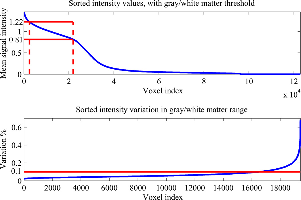
APPLECOR attempts to correct for the corrupting effect of globally consistent, non-neural signals in fMRI data. A calibration volume that will best facilitate estimation of these signals is selected from each data set. We focus on correcting for global noise affecting brain areas of neural activation, which will be the gray matter and possibly white matter. Signal variation in gray matter is generally greater than signal variation in white matter, but physiological effects may be present in both regions. Cerebrospinal fluid (CSF) does not contain neurons and is not of interest when measuring activation or correlation. Edge voxels, which partially contain brain matter and partially contain air or CSF, will see large signal changes with small motion because of partial volume effects, which are not common to the rest of the brain. Therefore, for this study, calibration was limited to gray and white matter, which were segmented from the images based on mean signal level. Intensity cutoffs were determined based on the second derivative of sorted intensity values. Sorting the mean signal intensity for all voxels revealed that gray matter and white matter were represented within an affine region of the curve for all data sets. An example of this sorted curve and the calculated thresholds is shown in the top of Fig. 1. Segmentation was verified by inspection for each subject. Edge voxels were removed from the calibration volume based on total signal variation. If the time course of a voxel’s signal varied by more than a specified threshold, the voxel was classified as an edge voxel and removed from the calibration volume. Variations greater than 0.1% of mean signal intensity were classified as an edge voxel, as that was found to be an appropriate threshold for each of the data sets in this study. An example showing the variation of each voxel in the white/gray matter intensity range, as well as the edge detector threshold, is shown in the bottom of Fig. 1. Inspection confirmed that the voxels removed by the edge voxel detector were nearly all at the periphery of the brain or the ventricles for each data set.

Figure 1.

Representative distributions used in white/gray matter segmentation. Top plot shows the sorted intensity values for all voxels in the data set. Solid red lines show the maximum and minimum intensity thresholds for gray/white matter. Bottom plot shows the sorted variation values for the gray/white matter voxels, with a red line showing the cutoff used in identifying edge voxels.

2.5 Signal Model

APPLECOR assumes that a voxel’s signal is the sum of a constant offset (mean signal over time), true neural BOLD modulation, additive physiological noise, multiplicative physiological noise, and thermal noise. Physiological corruption that is not additive will likely scale as a function of voxel mean intensity (Kruger & Glover, 2001) and of tissue properties such as gray/white matter content or vascularity (Bandettini & Wong, 1997), motivating the inclusion of the multiplicative term. The multiplicative term can capture some of the effects that are tied to tissue properties and vascularity, since the magnitude of such effects correlates with the mean signal intensity.

The APPLECOR signal model for voxel iis

$${\mathrm{V}}_{\mathrm{i}}(\mathrm{t})={\mathrm{\mu }}_{\mathrm{i}}+{\mathrm{B}}_{\mathrm{i}}(\mathrm{t})+{\mathrm{C}}_{1\mathrm{i}}*{\mathrm{P}}_{\text{add}}(\mathrm{t})+{\mathrm{C}}_{2\mathrm{i}}*{\mathrm{\mu }}_{\mathrm{i}}*{\mathrm{P}}_{\text{mult}}(\mathrm{t})+{\mathrm{P}}_{\mathrm{i}}(\mathrm{t})+{\mathrm{N}}_{\mathrm{i}}(\mathrm{t}),$$ (1)

where μ_i is the mean signal level for voxel i, B_i(t) is the neural-induced BOLD modulation that we hope to uncover in the recorded fMRI data, P_add(t) is the global additive noise, and P_mult(t) is the global multiplicative noise, representing factors discussed earlier. P_i(t) represents the aggregate effect of any other corrupting signals on voxel i that are not global. N_i(t) is zero-mean noise, which we assume to be Gaussian for high signal intensities. If the additive and multiplicative physiological effects are perfectly consistent across the brain volume and across tissue types, then the constants C_1i= C_2i = 1. However, if there are spatial differences in susceptibility to physiological effects then these constants will allow for amplitude scaling of the physiological confounds. The P_add and P_mult terms are what APPLECOR attempts to estimate and remove from the fMRI data.

2.6 Estimation of Physiological Noise

The APPLECOR algorithm attempts to determine P_add(t) and P_mult(t) and subsequently project them out of the data by using them as nuisance regressors in a GLM. As a first step, mean signal values are removed from each calibration voxel’s time course. This leaves

$${\mathrm{R}}_{\mathrm{i}}(\mathrm{t})={\mathrm{V}}_{\mathrm{i}}(\mathrm{t})-{\mathrm{\mu }}_{\mathrm{i}}={\mathrm{B}}_{\mathrm{i}}(\mathrm{t})+{\mathrm{C}}_{1\mathrm{i}}*{\mathrm{P}}_{\text{add}}(\mathrm{t})+{\mathrm{C}}_{2\mathrm{i}}*{\mathrm{\mu }}_{\mathrm{i}}*{\mathrm{P}}_{\text{mult}}(\mathrm{t})+{\mathrm{P}}_{\mathrm{i}}(\mathrm{t})+{\mathrm{N}}_{\mathrm{i}}(\mathrm{t})$$ (2)

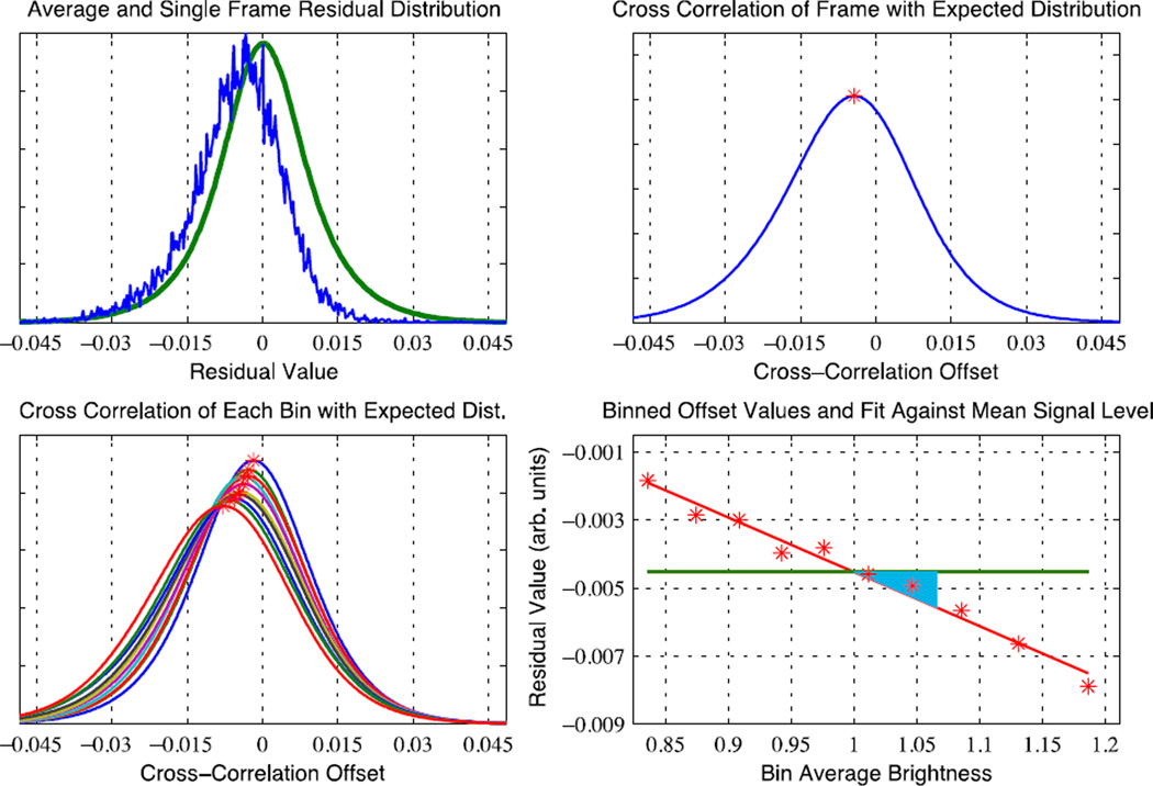
as the residual signal of each voxel. Empirically, the distribution of R_i(t) values across space (within the calibration volume) or across time gives approximately Gaussian distributions. The time-averaged spatial distribution will be referred to as the “expected distribution” of residual values. This distribution is a mixture of the N, B, and P distributions. Looking at an individual time frame j, the distribution of residual values across voxels should look similar to the expected distribution. If P_add(j) = P_mult(j) = 0, and the average (across voxels) of B_i at frame j is 0, then the distribution of R_i(j) will be centered on zero. If there is an additive offset, P_add(j) • 0, the distribution of R_i(j) will be centered on P_add(j), (assuming that C_1i = 1 for all i.)If P_mult(j) • 0, then the center of the distribution for a subset of voxels will depend on their mean values. In order to determine the additive and multiplicative offsets together, the calibration voxels are first binned according to mean signal intensity, μ_i. Using ten bins was found to be a suitable tradeoff between robustness and precision. For each time frame, the distribution of residuals for each bin is cross-correlated with the expected distribution to find the offset that yields the maximum cross-correlation. (This offset is the best estimate of the center of the distribution within that bin.) These offsets are then plotted against the mean signal intensity of each bin and an affine fit is computed. The affine fit parameters are APPLECOR’s initial estimate of P_add(j) and P_mult(j), with the slope being P_mult(j) and the y-intercept being P_add(j).

The stages of correction thus far are referred to as APPLECOR0, as they are the foundation of and the first pass for the APPLECOR algorithm. An example of distribution comparisons, cross-correlations, and fit is shown in Figure 2. After execution of APPLECOR0, we have an initial estimate of P_add(t) and P_mult(t). However, additional adjustments are necessary. First, we note that small errors in the multiplicative estimate lead to substantial error in the additive estimate. Since the y-intercept measures the offset for a zero mean signal, errors in the 1^st order term are magnified by the offset between the mean intensities and zero. In order to make the additive offset more accurately reflect the additive bias in the brain, we adjust the model such that the estimated additive signal is considered to be A_est(t) = [P_add(t) + P_mult(t)*mean(μ_i)] instead of just P_add(t), where mean(μ_i) is the average mean signal intensity throughout the calibration volume. We can also redefine our scaling constants to absorb the modified designation. This gives a new formula for the residuals,

$${\mathrm{R}}_{\mathrm{i}}(\mathrm{t})={\mathrm{B}}_{\mathrm{i}}(\mathrm{t})+{\mathrm{C}}_{3\mathrm{i}}*{\mathrm{A}}_{\text{est}}(\mathrm{t})+{\mathrm{C}}_{4\mathrm{i}}*{\mathrm{P}}_{\text{mult}}(\mathrm{t})+{\mathrm{P}}_{\mathrm{i}}(\mathrm{t})+{\mathrm{N}}_{\mathrm{i}}(\mathrm{t})$$ (3)

where C_3i and C_4ihave absorbed other constants and will not be equal to one. The newly defined additive estimate, A_est(t), gives the expected global noise time course for a voxel of average intensity. This term is also a more robust estimate of global additive offset than simply taking the global mean, since outliers are given less weight in cross-correlation instead of being given equal weight as in global mean calculation. Second, we want to calibrate for estimates of the global noise parameters only in voxels in which global noise is significant. If the neural signal B_i(t) dominates, or if C_1i or C_2i are significantly different than 1, inclusion of the voxel i in calibration may bias our noise estimate. To increase the likelihood that only voxels with significant, common physiological noise are included in calibration, the calibration volume is restricted to voxels with a strong positive correlation with the initial noise estimate A_est(t). A threshold of Pearson correlation r•0.15 was chosen, as it empirically gave the most consistent DMN results across different testing parameters. This threshold preserved 55% of the original calibration volume on average, with a standard deviation of 12%, when processing the full duration of each of the fifteen data sets.

Figure 2.

Illustration of histograms and APPLECOR0 fits for a single frame of fMRI data. Top left shows the distribution of residual in calibration voxels (blue) and the average distribution across time (green). The cross-correlation of these distributions is shown top right, with a red star marking the maximum. Bottom left shows the cross-correlations and maximums for the same frame, separated into 10 bins according to magnitude. Bottom right shows the maximums plotted against bin intensity, with the APPLECOR0 A_est(green) and multiplicative (blue triangle) fits.

APPLECOR0 is run again with the reduced calibration volume to produce improved estimates of A_est(t) and P_mult(t). Finally, a GLM is run with A_est(t), P_mult(t), and the 0^th, 1^st, and 2^nd powers of time as nuisance regressors to remove all estimated corruption from all voxels. Ideally, this full implementation of APPLECOR will leave only V_i,APPLECOR = B_i(t) + P_i(t) + N_i(t) after correction. APPLECOR can also be combined with other GLM-based corrections by using additional nuisance regressors. “PEARCOR”, or Parallel Execution of APPLECOR and RVHRCOR, uses the estimated physiological regressors from APPLECOR and from RVHRCOR together in a GLM to remove as much physiological corruption as possible. All processing and analysis in this study was performed using MATLAB (2010a, The Mathworks, Natick, MA).

2.7 Temporal Consistency

The seven 16-minute resting state fMRI data sets were used to analyze the temporal stability of the DMN after various corrections. Each data set was prepared by first applying RETROICOR, then performing slice-timing correction (alignment of the 2D slices to make temporally consistent volumes), and finally applying one of the following corrections: None, RVHRCOR, global mean regression (hereafter referred to as “GMR”), APPLECOR, PEARCOR. Each correction approach was also tested without application of RETROICOR. After correction, the data sets were split into 2-minute time windows, with successive windows slipped forward every 1 minute to create 15per scan. These windows included the breath hold period for subjects that performed that task, as insensitivity to breathing is a desirable trait for the corrections. A seed ROI from the posterior cingulate cortex (PCC), which is a central node of the DMN (Greicius et al., 2003; Greicius and Menon, 2004; Raichle et al., 2001) was defined for each subject by normalizing the MNI standard-space ROI ((5mm-radius sphere, centered at (x = −6, y = −58, z = 28)) to that subject’s mean functional image. Within each time window, the Pearson correlation between each voxel and the average time signal in the PCC ROI was calculated. Correlation coefficients were converted to Fisher Z values. Temporal consistency at each voxel was measured as the standard deviation, across time bins, of Fisher Z values.

2.8 Inter-subject Consistency

All 15 fMRI data sets were used to analyze the consistency of DMN across subjects before and after correction. To avoid inconsistency from the differing scan times and from the initial breath holds, only the last 8 minutes of each subject’s data set were considered in this analysis. Each of the following correction methods was then applied for comparison, both with and without first performing RETROICOR: None, RVHRCOR, GMR, APPLECOR, PEARCOR. After applying each correction, the correlation between each voxel and the average time signal in the PCC ROI was calculated. Correlation coefficients were converted into Fisher Z statistics, and the resulting maps were normalized into MNI space, and the normalized correlations maps were submitted to a group-level one-sample t-test using SPM5 (http://www.fil.ion.ucl.ac.uk/spm). A nuisance factor of “scanner” was included to account for subjects having been scanned on 1 of 2 different scanners. In addition, for each correction approach, consistency across subjects was calculated for each standard-space voxel by taking the standard deviation of normalized voxel correlation across subjects.

2.9 Network Stability Simulation

In order to analyze the effects of the corrections in a more controlled setting, simulations were performed by injecting artificial resting state networks into recorded data. For each iteration of the simulation, one of the seven 16 minute data sets was selected at random. A sinusoid with random starting phase and a random period (uniform over [26, 34] seconds) was created as a synthetic injection signal. Ten percent of the calibration voxels were chosen at random as injection sites, and the sinusoid was added to their time courses. Amplitude of the injection signal was set to 0.1% of the average calibration voxel intensity, which gave a typical mean correlation in the injection volume with significance p•0.0015. Three hundred iterations were performed. For each iteration, temporal consistency was analyzed as was described earlier for the measured data. The mean correlation (with the sinusoid) across time was calculated for each voxel, and the correlation coefficients were then averaged within the injection and non-injection volumes. The standard deviation of correlation across time was found to be consistent across the injection and non-injection sites, so the standard deviation across time of all calibration voxels was averaged. The average across trials for each parameter was calculated, as well as the standard deviations, to determine statistical significance of the results.

2.10 Comparison Between Regressed Signals

In order to quantify similarity or dis-similarity between the corrections, correlations between the regressed signals were measured. RVHRCOR, GMR, APPLECOR, and PEARCOR were run on the seven 16-minute data sets, extracting only the signals that were regressed out by the various approaches (i.e., the first- and second-order trend terms were not included in these extracted signals). The correlation between the extracted signals for every pair of approaches was computed for every voxel in every subject. These correlations were averaged across gray and white matter within each subject to yield a metric assessing the similarity of regression between the correction approaches for each of the 7 subjects.

2.11 Correction Bias Simulation

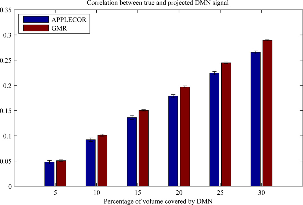
There is a concern that if resting state networks are large, their true neural fluctuations will influence the estimated noise regressors for the data-driven corrections (GMR, APPLECOR, and PEARCOR). We therefore performed simulations to gauge the degree to which these correction methods are susceptible to bias from neurally-based network activity. In our simulated set of voxels, a fixed fraction of the voxels shared a common underlying signal and thus formeda network (the “DMN”),and the remaining voxels contained only random Gaussian noise. Time series were generated from Gaussian white noiseto serve as global additive and multiplicative noise, and were added to all voxels. Thermal Gaussian noise of fixed amplitude was generated and added to all voxels. A “true DMN” random Gaussian signal was created that was orthogonal to the additive and multiplicative time series, and variation across voxels within the DMN was created by multiplying the true DMN time series by the absolute value of random Gaussian time series prior to being added to the noise signals. In order to generate appropriate parameters for the simulation, data from subject 1 was used. The distribution of mean signal intensities were taken from the gray and white matter in this data set, with the “DMN” voxels being selected uniformly across all intensities. The variance of the additive and multiplicative signals were selected to match the average estimated additive and multiplicative variances from the APPLECOR GLM of subject 1. The true DMN signal was made orthogonal to the additive and multiplicative signals so that any measured correlation between them after correction could be attributed to bias from the correction. The variance of the true DMN signal was selected to match the average estimated PCC signal in voxels that had r>0.20 correlation with the PCC after APPLECOR correction. Prior to adding the additive and multiplicative noise, the mean correlation between voxels in the simulated DMN was 0.27, which was the average correlation with the PCC in subject 1 for significantly correlated voxels after APPLECOR. The fractional volume of the DMN was varied from 5% to 30% in 5% steps, with 30 iterations of the simulation run at each fractional volume. To measure the amount of correlation between the estimated regressors and the true DMN signal, the true DMN was projected onto the GMR regressor or simultaneously onto the APPLECOR additive and multiplicative regressors, and the correlation between the true DMN and the projected DMN was calculated for each correction method.

3. Results

3.1 Consistency of Residuals

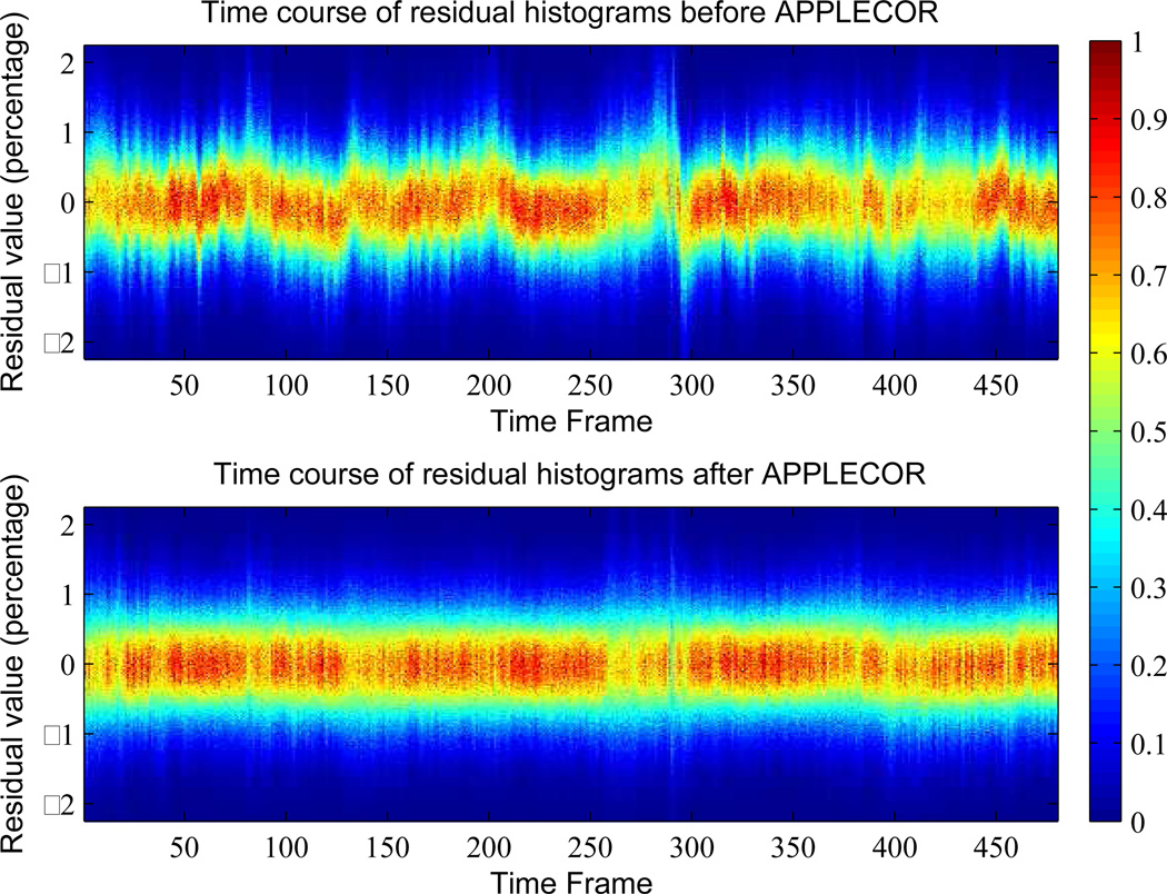
One of the assumptions implicit in APPLECOR is that the distribution of residual values within a data set is stable across time after accounting for additive or multiplicative biases. In order to test this assumption, histograms of the distribution of residual values for each frame were computed before and after correction. An example of the distribution of residual values across time for a sample resting state data set before and after APPLECOR correction is shown in Fig. 3. The amount of and type of variation in the distributions before correction differ across data sets. The distribution time history after correction shown in Fig. 3 is representative of six of the seven 16-min data sets after correction, while the other subject’s distribution time history varied slightly more.

Figure 3.

Distributions of residual values (as a percentage of mean intensity) across time before (top) and after (bottom) application of APPLECOR. First and second order trends have been removed in each case.

3.2 Temporal Consistency Results

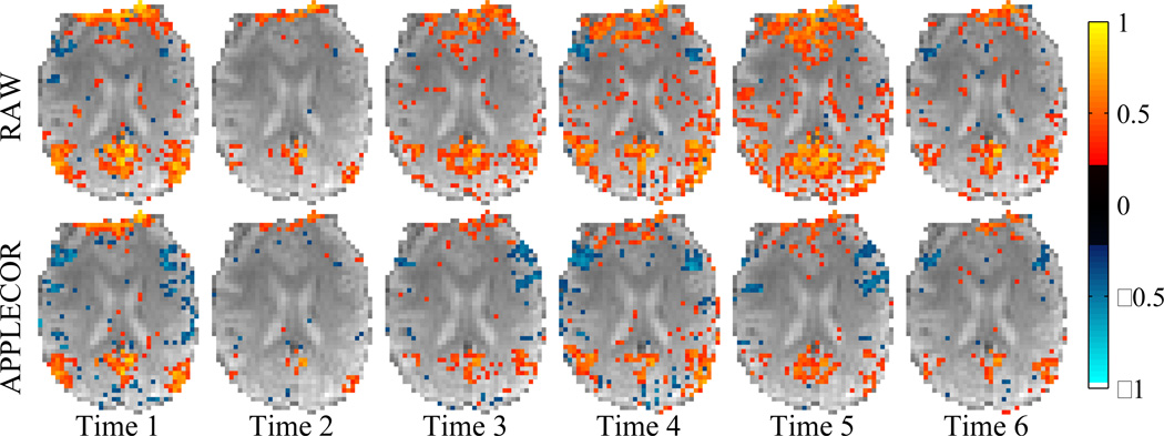
Temporal consistency analysis on the seven 16-minute data sets produced 15 time bins of correlation for each subject with each correction approach. Figure 4 shows, for one subject, the first 6 non-overlapping time bins for a representative slice that includes the PCC, both with and without APPLECOR. (For the data in this figure, RETROICOR has not been applied.)Each frame is presented in the same color scale, with gray-scale representing the underlying average signal. Color is overlaid to indicate correlation with the PCC, thresholded at significance p<0.01 (not corrected for multiple comparisons).

Figure 4.

Correlation with the PCC across time bins for subject 1 within a slice that includes the PCC: without (top) and with (bottom) APPLECOR.

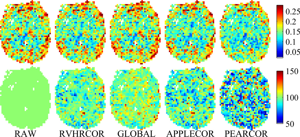
Consistency across time was measured using the standard deviation of Fisher z scores for correlation with the PCC across the 15 time bins. Figure 5 shows a map of temporal standard deviation for a single slice in a single subject, using each of the correction approaches. Figs. 4 and 5 show the same slice from the same subject. Lower temporal standard deviation indicates greater stability of the measured DMN over time. Lower spatial variation of temporal consistency indicates more consistent remaining noise throughout the brain.

Figure 5.

Temporal standard deviation of correlation with PCC after various corrections, shown for a single representative subject. Top row shows the temporal variation for each voxel. Bottom row shows the percentage of the raw variation by voxel, normalized to that of the raw data.

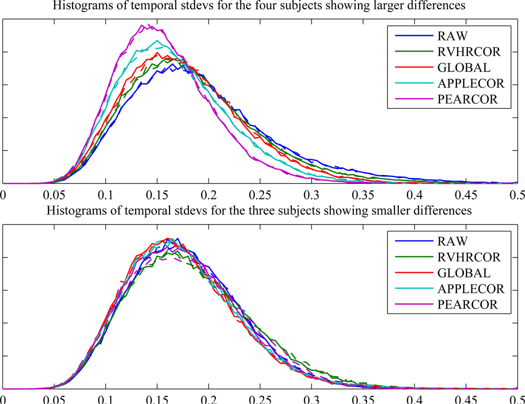
In an attempt to quantify the effects of the various corrections on temporal consistency, the distribution of temporal standard deviations for all gray or white matter voxels was plotted for each subject. For three of the subjects, small differences were found in consistency between the corrections, while larger differences appeared between corrections for the other four subjects. The top of Fig. 6 shows the distribution of temporal standard deviations across the subjects showing large differences, and the bottom shows this data across only the three subjects showing smaller differences. The relative ordering of the histograms (across correction approaches) was consistent for the subjects showing larger differences, while the ordering of the correction histograms for subjects showing small differences was somewhat variable. Distributions closer to zero reflect greater consistency across time bins. Narrower distributions indicate greater consistency across space and subjects. To give a numerical representation, Table 1 shows the mean across subjects of the average temporal variation, as well as the spatial deviation of temporal variation after each correction. (These statistics are calculated across all voxels that have a signal intensity in the range spanned by gray and white matter. Percentages of the values found for uncorrected data are included for ease of interpretability.) In order to see subject-to-subject variation that may be disguised by population level statistics, Table 2 shows the average temporal variation after each correction, for each subject.

Figure 6.

Histograms of temporal standard deviations after various corrections for subjects showing larger changes (top) and smaller changes (bottom). Solid lines used RETROICOR, dashed lines did not.

Table 1.

Average statistics across seven subjects for temporal consistency. Third column shows the mean across subjects of the mean temporal standard deviation. The fourth column shows the average across subjects of the standard deviation across space of temporal standard deviations. Smaller values indicate improved consistency. Percentages shown are relative to the data on which no corrections were applied (first row).

Correction Applied	RETROICOR?	Average Temporal Standard Deviation	Spatial Standard Deviation of Temporal Standard Deviations
None	No	0.1853 (100%)	0.0580 (100%)
None	Yes	0.1852 (99.9%)	0.0575 (99.12%)
RVHRCOR	No	0.1822 (98.34%)	0.0556 (95.84%)
RVHRCOR	Yes	0.1818 (98.10%)	0.0549 (94.55%)
GMR	No	0.1757 (94.82%)	0.0540 (93.01%)
GMR	Yes	0.1748 (94.32%)	0.0537 (92.55%)
APPLECOR	No	0.1695 (91.44%)	0.0519 (89.48%)
APPLECOR	Yes	0.1690 (91.21%)	0.0510 (87.91%)
PEARCOR	No	0.1661 (89.64%)	0.0479 (82.51%)
PEARCOR	Yes	0.1642 (88.61%)	0.0470 (81.05%)

Table 2.

Average temporal consistency for each subject after applying each correction. Values are the mean (across space) of the temporal standard deviation of Fisher Z scores. Lower values indicate improved consistency. The boldface entries indicate the best consistency for each subject.

Subject	1	2	3	4	5	6	7
Raw	.1720	.1762	.2099	.1489	.2087	.1777	.2038
RETROICOR	.1707	.1760	.2110	.1502	.2053	.1772	.2057
RVHRCOR	.1728	.1774	.1996	.1451	.2237	.1653	.1917
RVHRCOR &RETROICOR	.1707	.1774	.2008	.1464	.2203	.1646	.1921
GMR	.1649	.1765	.1839	.1448	.2031	.1794	.1775
GMR&RETROICOR	.1627	.1759	.1842	.1452	.2022	.1773	.1759
APPLECOR	.1612	.1764	.1594	.1414	.2024	.1686	.1768
APPLECOR &RETROICOR	.1594	.1761	.1605	.1427	.2004	.1675	.1767
PEARCOR	.1613	.1816	.1576	.1418	.2105	.1474	.1625
PEARCOR&RETROICOR	.1543	.1793	.1599	.1416	.2021	.1478	.1645

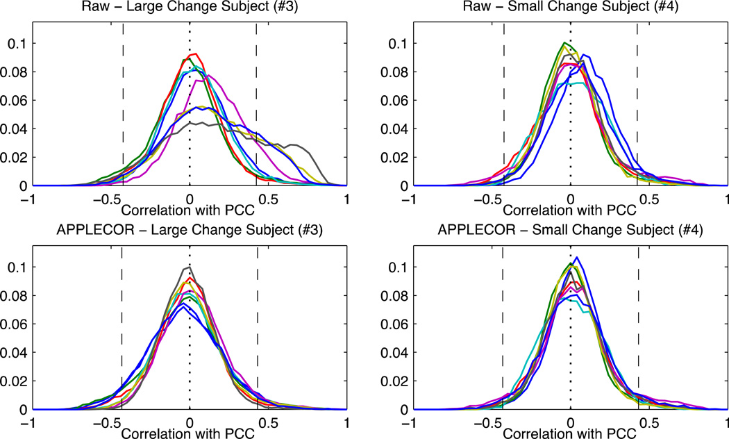
In order to visualize how the overall distribution of correlations changes with time, Figure 7 shows the distribution of correlations with the PCC in two of the subjects before correction and after APPLECOR. Only the 8 non-overlapped time windows are displayed (each is a different color), and single measurement p<0.001 thresholds are overlaid. The subject shown on the left was one of the subjects showing a large difference after correction, while the subject on the right showed smaller differences. (In Table 2, these are subjects 3 and 4 respectively.)

Figure 7.

Distributions of correlation values, across 2-minute time windows. The first row shows distributions after only 1st and 2nd order trend regression, while the bottom row used APPLECOR. The subject in the left column showed larger differences in consistency after correction, the subject on the right showed smaller differences. Vertical dashed lines indicate p<0.001 (uncorrected for multiple comparisons).

3.3 Group Level Consistency Results

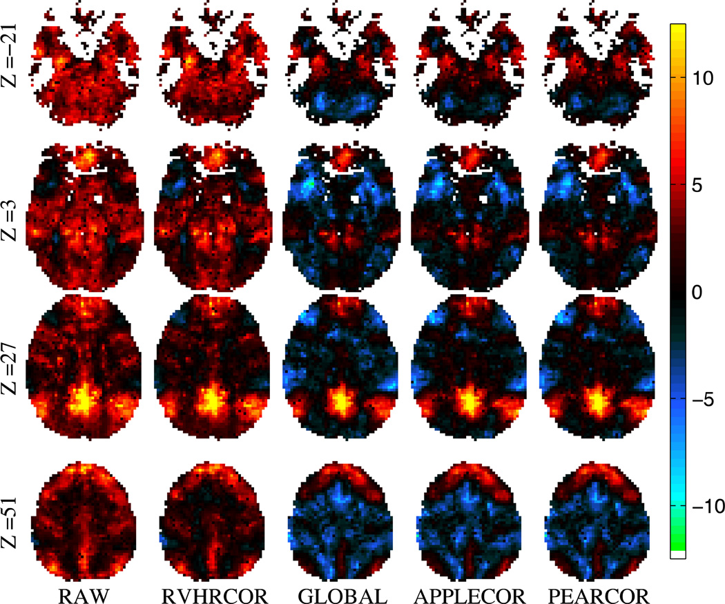
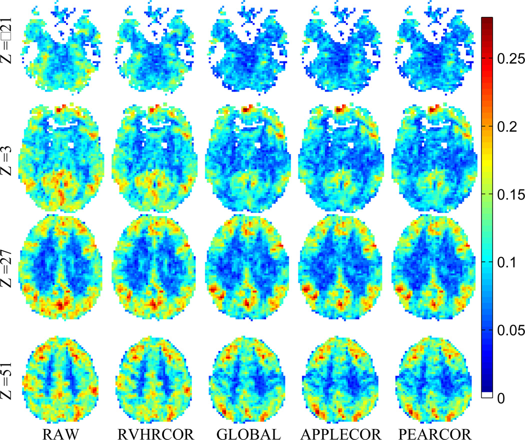
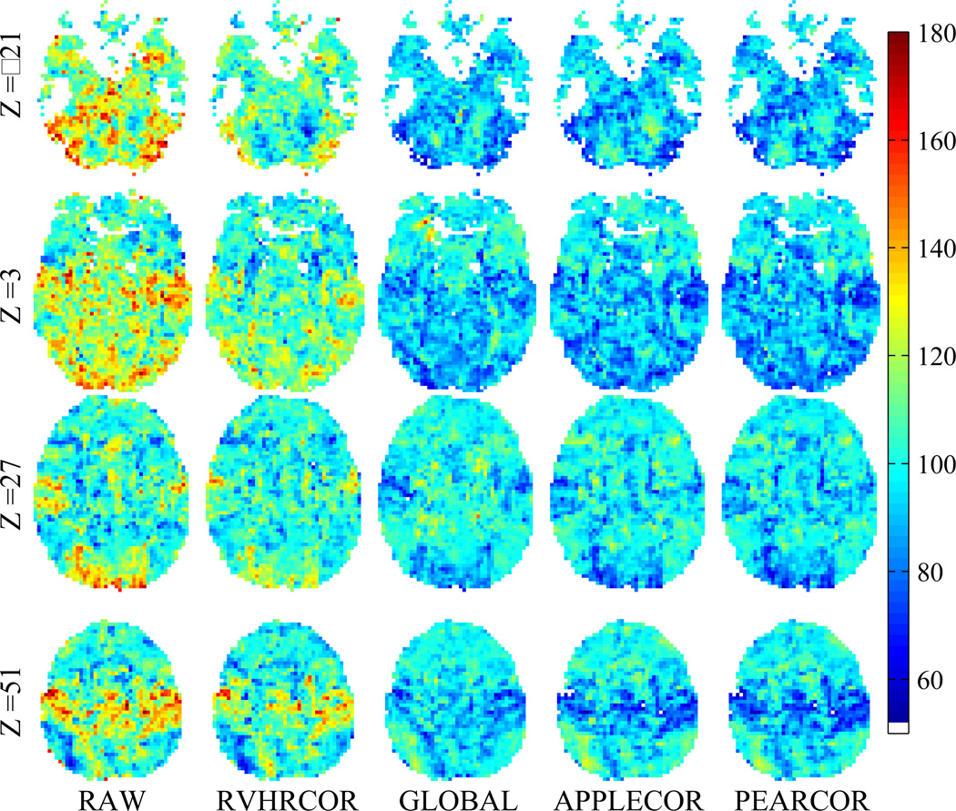
Group-level analysis of functional connectivity with the DMN seed region was performed across the 8-mindata sets of 15 subjects. Group-level t scores for 4representative slices are shown in Fig. 8.The slices shown are axial slices at MNI coordinates z=−21, 3, 27, 51. In addition, consistency for each normalized voxel was measured using the standard deviation of correlations across the subjects. This standard deviation across subjects is shown in Figs. 9 and 10 for the same slices as shown in Fig. 8. (The data in Figs. 9 and 10 is the same, but Fig. 10 has been normalized per voxel to show greater contrast between corrections.) To give a numerical metric, the mean across space of inter-subject variation (standard deviation) was measured for each correction approach. As in the temporal comparisons, the spatial standard deviation was calculated as well. These values are provided in Table 3.

Figure 8.

Group level t-scores of functional connectivity with the PCC across 15 subjects, shown after performing the indicated corrections.

Figure 9.

Variation (standard deviation) of DMN correlation across subjects after various corrections. Single-subject maps were normalized to MNI space prior to computing the across-subject variation.

Figure 10.

Normalized variation of DMN correlation in MNI space across subjects after various corrections. (Normalization is such that average value across corrections is 100.)

Table 3.

Variation statistics across fifteen subjects in standardized coordinate system. Third column shows the mean across-subjects standard deviation. The fourth column shows the standard deviation across space of across-subject standard deviation. Smaller values indicate improved consistency. Percentages shown are percent of no-correction value.

Correctionm Applied	RETROICOR?	Average Across- Subject Standard Deviation	Spatial Standard Deviation of Across-Subject Standard Deviations
None	No	.1212 (100.0%)	.0399 (100.0%)
None	Yes	.1211 (99.93%)	.0402 (100.8%)
RVHRCOR	No	.1137 (93.87%)	.0386 (96.92%)
RVHRCOR	Yes	.1139 (94.03%)	.0391 (98.19%)
GMR	No	.1033 (85.24%)	.0380 (95.32%)
GMR	Yes	.1027 (84.73%)	.0385 (96.64%)
APPLECOR	No	.1021 (84.27%)	.0384 (96.42%)
APPLECOR	Yes	.1014 (83.66%)	.0389 (97.62%)
PEARCOR	No	.1005 (82.97%)	.0378 (94.78%)
PEARCOR	Yes	.0999 (82.46%)	.0382 (95.92%)

3.4 Network Stability Simulation Results

The measured parameters from the injected network simulation are summarized in Table 4. Lower temporal standard deviation of correlation with the injected signal indicates improved consistency of the correlation results. As can be seen in the far right column, all of the correction approaches improved consistency of the correlation values. Ideally, correlation with the injected signal would be maintained or increased by a correction approach, while correlation in the non-injection volume would be maintained or reduced (towards zero). Each of the correction approaches decreased the average correlation in the injection volume. GMR regression reduced it the most, by 5.2%, whereas RVHR only reduced it by 1.8%. Correlation in the non-injection volume was perturbed the most by GMR (changing r by approximately −0.015), followed by APPLECOR and then PEARCOR (each changing r by approximately 0.009). Separation of true correlations from false positives is improved if variation is reduced more than the mean is reduced. Only APPLECOR resulted in a greater reduction in temporal variation over average correlation in the injection for this particular strength of injected signal. Parameter differences between corrections were smaller than one across-trial standard deviation. Paired t-tests were run for each correction pairing and each parameter to measure statistical significance of differences. APPLECOR and PEARCOR were found to be significantly (p<<0.05 for most pairings, p<0.06 in the least significant case) different than no correction and RVHRCOR for each parameter. APPLECOR and PEARCOR were not strongly significantly different than GMR for the parameters.

Table 4.

Summary of trial averages from network simulation. Percentages are fraction of the parameters in the raw data.

Correction Applied	Average Non- Injection Correlation	Average Injection Correlation	Across-Trial Standard Deviation of Correlation Means	Average Temporal Standard Deviation	Across-Trial Standard Deviation of Temporal Standard Deviations
None	−0.0004	0.1676 (100%)	0.0169	0.2286 (100%)	0.0238
RVHRCOR	0.0002	0.1646 (98.2%)	0.0178	0.2256 (98.7%)	0.0201
GMR	−0.0149	0.1569 (93.6%)	0.0052	0.2206 (96.5%)	0.0193
APPLECOR	−0.0092	0.1623 (96.8%)	0.0061	0.2191 (95.9%)	0.0180
PEARCOR	−0.0088	0.1579 (94.2%)	0.0066	0.2179 (95.3%)	0.0175

3.5 Comparison Between Regressed Signals Results

Correlations were calculated between the signals that were regressed out of the data for each pair of correction approaches. These correlations were averaged across gray and white matter within each subject, and the results are tabulated in Table 5.

Table 5.

Average correlations between signals regressed out of the data by each pair of correction approaches. The first two columns indicate the correction approaches compared, with the first row indicating the subject number.

		1	2	3	4	5	6	7
RVHRCOR	GMR	.170	.103	.198	.046	.271	.326	.272
RVHRCOR	APPLECOR	.143	.112	.154	.097	.286	.311	.228
RVHRCOR	PEARCOR	.476	.465	.435	.404	.421	.562	.447
GMR	APPLECOR	.663	.547	.582	.573	.546	.663	.668
GMR	PEARCOR	.589	.493	.529	.534	.514	.592	.614
APPLECOR	PEARCOR	.868	.868	.891	.903	.934	.866	.907

3.6 Correction Bias Simulation Results

For each iteration of the simulation, the correlation between the true DMN signal and the projected DMN signal was calculated for each of the corrections (GMR and APPLECOR). At each fractional DMN volume size, 30 iterations of the simulation were run, and the mean correlation and standard error of the mean correlation were calculated for each correction. These results are shown in Figure 11. At each fractional volume, the average correlation for each correction is shown, along with error bars indicating ±3 standard errors. Lower correlations indicate less bias and lower likelihood of removing desired neural signal. Paired t-tests were significant at each DMN extent, ranging from p<0.007 for 5% extent to p<4e-21 for 30% extent.

Figure 11.

Mean correlation between true DMN signal and the DMN signal projected on estimated regressors from GMR and APPLECOR. Lower values are better, as they indicate a decreased likelihood of removal of neural signal. Error bars indicate ±3 standard errors.

4. Discussion

We have introduced a method for estimating and removing non-neural noise from fMRI recordings, and have examined its impact on temporal, spatial, and inter-subject consistency of the DMN in resting-state connectivity analysis. Although the DMN is not expected to be perfectly constant across time and across subjects (Chang and Glover, 2010), it is expected to be more stable than it appears in raw recordings. An ideal correction would remove as much non-neural signal as possible, while preserving true temporal variations in neural activity and connectivity. If a noise correction method increases the DMN stability, it is a strong indication that the correction is correctly removing non-neural noise from the data. Results show that the new corrections result in greater DMN stability than alternative corrections (or no correction) consistently across subjects and measures of consistency. PEARCOR, followed by APPLECOR, attained the greatest consistency of the DMN as measured across time and across subjects, and the variation of these parameters across space was also lowest for the new corrections. Results from simulation were ordered similarly to results from measured data, but the measured differences were much smaller. The simulation did not refute any of the observed consistency improvements, while it also did not reveal any compelling insight.

4.1 Consistency of Residuals

The residual distributions are very consistent after APPLECOR, which supports the algorithm’s underlying signal assumptions of consistent neural distributions with inconsistent non-neural signals. Additionally, we posit that changes in the distribution of residuals between time frames may indicate changes in data quality. For example, in Fig. 3, there are clearly some frames interspersed through the data that have a wider distribution of residuals. These frames may indicate subject motion or other irregular corruption of the signal. While further investigation of this phenomenon is required, it is possible that using the within-frame variance as a data quality metric may allow for better correction results by introducing a confidence weighting when estimating or removing physiological signals or calculating network connectivity correlations.

4.2 Calculation of Global Mean Offset

Comparison between the APPLECOR algorithm and GMR suggests that APPLECOR using only a single intensity range bin per frame to estimate A_est(t) estimates global noise better than GMR. If there is a global additive bias to the brain signal, the distribution of residual values [V_i(t) – μ_i] will be centered around that additive offset. Using cross-correlation with the expected distribution, APPLECOR will determine the additive offset with high accuracy. Because global mean calculation weights all voxels equally, voxels that have true activation or that happen to have outlying noise will contribute to calculation of the mean to the same degree as other voxels. APPLECOR, by virtue of cross-correlation, gives outlying voxel residuals less weight when estimating the underlying additive offset. Thus, APPLECOR is expected to be more robust than the global mean in measuring additive offsets in the presence of noise or true activations.

4.3 Temporal Consistency

APPLECOR increased the temporal consistency of resting-state correlations more than RVHRCOR or GMR for most of the long (16-min) data sets, regardless of whether RETROICOR was also applied. Compared to the raw data, temporal variation (as measured by standard deviation) was reduced on average by 8.5% with APPLECOR, while PEARCOR (coupled with RETROICOR) reduced it by 11.4%. RVHRCOR and GMR reduced temporal variation by 1.9% and 5.7% respectively when paired with RETROICOR. The margins by which APPLECOR or PEARCOR outperformed RVHRCOR or GMR were several times larger than the margins by which APPLECOR or PEARCOR were outperformed. These results indicate that APPLECOR and PEARCOR improve the temporal consistency across most subjects, and that the group level results are not driven by outliers. Spatial variation of the temporal consistency was also reduced when using APPLECOR, and even more so when using PEARCOR. Spatial variation of temporal consistency was reduced by 10.5% using APPLECOR alone and by 19.1% using PEARCOR with RETROICOR. RVHRCOR and GMR reduced spatial variation by 4.2% and 7.5% respectively when paired with RETROICOR. In all cases, application of RETROICOR before other correction approaches improved the temporal consistency of DMN correlations. These results further suggest that some of the temporal variation generally seen in the DMN may be artifactual.

A particular feature of the temporal consistency is apparent when browsing through time windows, but is not captured by the numeric metrics presented in the Results section. In most of the subjects, there are time frames in which most of the brain becomes significantly correlated with the PCC in the raw data. This large-scale correlation indicates large-scale noise dominating the underlying neural activation. Subjectively, in frames where this is the case, APPLECOR and PEARCOR suppress the large-scale correlation, but they also reduce the volume of significant correlations in regions where correlation is expected. This effect is somewhat visible in Fig. 4. It is not certain which of these outcomes is preferable, but it appears that the use of APPLECOR or PEARCOR will significantly reduce the likelihood of false positive correlations in resting state analysis, possibly at the expense of reduced detectability (true positives).

Figure 7 shows a comparison of PCC correlations in 2-minute windows from two of the subjects. An initial observation of this figure reveals that the APPLECOR distributions are all centered near zero and appear somewhat Gaussian. If the majority of the brain voxels are unconnected to the PCC, this would be expected. Many of the raw 2-minute distributions are also centered around zero and appear somewhat Gaussian, but some of the distributions are not. In particular, the subject that showed large increases in consistency after correction had several time windows that showed a significant positive correlation bias and spread of correlation values. These results are consistent with the theory that widespread physiological noise introduces artificial positive correlations, and that APPLECOR attempts to reduce them by regressing out estimated non-neural contributions. These plots also suggest that the reason that some subjects show little change in consistency after correction is that they were not very corrupted by non-neural noise to begin with. It is conceivable that future correction approaches may want to compare measured correlation histograms with an expected distribution to assess data quality.

4.4 Group Level Consistency

Group-level results show greater consistency across subjects after application of APPLECOR or PEARCOR. Some of the brain regions that are negatively correlated with the DMN after application of GMR also appear negatively correlated after application of APPLECOR or PEARCOR, suggesting that some of these regions are truly negatively correlated and not simply an artifact introduced by GMR. In particular, the task-positive network appears to be anti-correlated after any of these corrections. Variability across subjects was highest at the boundaries of the PCC, but close examination of the individual DMN results in native subject (acquisition) space suggests that much of this variability is due to mis-registration errors in the coordinate transformation to MNI space. The comparative ranking of the various inter-subject metrics is the same as was found in the temporal case. PEARCOR yields the most consistency across subjects, followed by APPLECOR, GMR, RVHRCOR, and no correction. In some cases, RETROICOR slightly improves consistency and in others it slightly decreases consistency. Similar to the temporal consistency results, the inter-subject consistency results suggest strongly that APPLECOR alone will produce more consistent (and potentially more accurate) correlations than will previously developed correction approaches, and that PEARCOR outperforms APPLECOR if physiological recordings exist to permit its use.

4.5 Network Stability Simulation

When injecting a known signal into a volume of resting state data, small but statistically significant differences in network strength and consistency were obtained across the various correction approaches. Interestingly, each of the corrections reduced the strength of correlation with the sinusoid in the injection volume, which is undesired. GMR created the greatest negative bias in correlations throughout the brain, which is expected since GMR assumes a zero sum model and must decrease all correlations if positive correlation are introduced (Murphy et. al, 2009). APPLECOR and PEARCOR also added negative bias to all correlations, but to a lesser extent than GMR. The amount to which the bias occurs will depend on the time history of the activation signal and its spatial extent, as the APPLECOR0 noise estimation gives less weight to stronger activation. The relative results of the various corrections were very dependent on simulation parameters, and it is not clear how representative the simulations are of actual recordings. In particular, the histograms of residuals in a time frame for the simulated data do not look similar to the histograms in actual measured data, so the additive sinusoid model may be deficient. Also, the differences between the consistencies after various corrections are much smaller with the simulated data than with the measured data, further suggesting that the simulation is not capturing the true effects of the corrections.

4.6 Similarity Between Regressors and Bias from Large Networks

It is well known that GMR can distort true correlation patterns, since the global mean signal contains an unknown mixture of neurally-based BOLD fluctuations along with noise (Murphy et al. 2009, Saad et al. 2012). Unfortunately, since it is impossible to truly disentangle meaningful signal from noise in resting state scans, all data-driven noise estimates obtained from gray-matter voxels may be biased to some degree by the presence of real correlations amongst brain regions (i.e. networks). We performed simulations in order to examine the relative degree to which the APPLECOR and GMR noise estimates are biased by the presence of large-scale networks. It was found that APPLECOR appears to suffer from significantly less bias compared to GMR across a range of simulated network volumes (5% – 30%), and therefore represents an improvement. We furthermore examined the degree to which the APPLE/PEARCOR noise estimates resembled the global signal within the actual fMRI data, and observed that the amount of shared variance ranged between 29.8% – 44.6% for APPLECOR (24.3% – 37.7% for PEARCOR); this, taken together with the significantly improved temporal consistency achieved by APPLE/PEARCOR compared to GMR, suggests that the proposed method is distinct from GMR and may contribute more than simply an incremental improvement.

4.7 Caveats, Limitations, and Future Work

True large-scale activations in the brain can bias APPLECOR’s noise estimates. To apply APPLECOR to task-based or sensorimotor fMRI data, it may be sufficient to exclude potential regions of activation from the calibration volume to avoid this bias. Further work will be necessary to determine the suitability and proper application of APPLECOR-like methods to non-resting-state data. Further investigation into the amount of bias introduced to resting-state data sets by APPLECOR is also warranted. Here, we address this issue by simulating the presence of a large-scale network and examining the degree to which the APPLECOR and GMR noise estimates are biased by the common temporal activity within the network. While we believe our simulation incorporated reasonable assumptions, as well as parameters derived empirically from an fMRI dataset, the simulated conditions are likely an oversimplification of realistic resting-state data.

Although the proposed corrections outperformed all of the alternatives at the group level, individual subjects sometimes showed slightly worse performance metrics after the proposed corrections as compared to the raw data or to other corrections. The difference between the performance metrics before and after corrections also varied greatly across the data sets. Figure 6 shows this effect very clearly. One situation that can lead to small differences between pre- and post- correction results would be if there were very little physiological corruption in the original data set, a scenario that is suggested for some data sets by Figure 7. Alternatively, if physiological noise manifested as a spatially heterogeneous factor rather than as a global component, the assumptions of our model would be violated. For one of the seven long data subjects (subject 5 in Table 2), variation remained high after correction suggesting that none of the corrections adequately removed non-neural corruption and that a more sophisticated approach may be necessary.

Another approach to removing the estimated physiological noise is to subtract [P_add(t) + μ_i * P_mult(t)] from each voxel’s signal rather than regressing it out in a GLM. The advantage to this approach would be that correlation between a true B_i(t) and the physiological signal would not result in removal of true neural signal during correction, beyond what was included in the estimate of A_est(t).The disadvantage would be that C_1i and C_2i would either need to be assumed constant (equal to 1.0) or estimated by some other means. Also, if the calibration volume included both white matter and gray matter, it would be likely that the strength of the estimated physiological noise would fall in between the true physiological noise for the two types of tissue. Therefore, it may be necessary to restrict the calibration volume to only the tissue type of interest. The subtraction (instead of regression) approach was evaluated using the full white and gray matter volume and found to be inferior to regression when analyzing resting state networks by all of the methods presented here.

5.Conclusions

A new data-driven correction method, APPLECOR, was developed for reducing non-neural signals in resting-state fMRI. In our data, APPLECOR reduced the amount of temporal and inter-subject variation in seed-based DMN correlations by more than alternative correction approaches (such as global mean regression). Assuming that non-neural components of the fMRI time series introduce artificial variation in DMN correlations, the observed improvement in consistency provides an indication that APPLECOR may effectively reduce non-neural signals in resting-state data. Since APPLECOR requires only the fMRI data as an input, it can be applied to scans for which no physiological monitoring was recorded. The combination of APPLECOR and RVHRCOR regressors (“PEARCOR”), which can be used when concurrent respiratory and cardiac measurements are available, was found to produce even greater consistency. We also observed that regions of the task-positive network were negatively correlated with the DMN after our proposed corrections, suggesting that these negative correlations are neural in origin if, as believed, the new corrections are properly regressing out non-neural signal.

References

- Bandettini PA, Wong EC. A hypercapnia-based normalization method for improved spatial localization of human brain activation with fMRI. NMR Biomed. 1997;10:197–203. doi: 10.1002/(sici)1099-1492(199706/08)10:4/5<197::aid-nbm466>3.0.co;2-s. [DOI] [PubMed] [Google Scholar]
- Beall EB, Lowe MJ. Isolating physiologic noise sources with independently determined spatial measures. NeuroImage. 2007;37:1286–1300. doi: 10.1016/j.neuroimage.2007.07.004. [DOI] [PubMed] [Google Scholar]
- Birn RM, Diamond JB, Smith MA, Bandettini PA. Separating respiratory-variation-related fluctuations from neuronal-activity-related fluctuations in fMRI. NeuroImage. 2006;31:1536–1548. doi: 10.1016/j.neuroimage.2006.02.048. [DOI] [PubMed] [Google Scholar]
- Biswal B, Yetkin FZ, Haughton M, Hyde JS. Functional connectivity in the motor cortex of resting human brain using echo-planar MRI. Magn. Reson. Med. 1995;34:537–541. doi: 10.1002/mrm.1910340409. [DOI] [PubMed] [Google Scholar]
- Chang C, Glover GH. Relationship between respiration, end-tidal CO2, and BOLD signals in resting-state fMRI. NeuroImage. 2009;47:1381–1393. doi: 10.1016/j.neuroimage.2009.04.048. [DOI] [PMC free article] [PubMed] [Google Scholar]
- Chang C, Cunningham JP, Glover GH. Influence of heart rate on the BOLD signal: the cardiac response function. NeuroImage. 2009;44:857–869. doi: 10.1016/j.neuroimage.2008.09.029. [DOI] [PMC free article] [PubMed] [Google Scholar]
- Chang C, Glover GH. Time-frequency dynamics of resting-state brain connectivity measured with fMRI. NeuroImage. 2010;50:81–98. doi: 10.1016/j.neuroimage.2009.12.011. [DOI] [PMC free article] [PubMed] [Google Scholar]
- Desjardins AE, Kiehl KA, Liddle PF. Removal of confounding effects of global signal in functional MRI analyses. NeuroImage. 2001;13:751–758. doi: 10.1006/nimg.2000.0719. [DOI] [PubMed] [Google Scholar]
- Fox MD, Snyder AZ, Vincent JL, Corbetta M, Essen DCV, Raichle ME. The human brain is intrinsically organized into dynamic, anticorrelated functional networks. Proc. Natl. Acad. Sci. U. S. A. 2005;102(27):9673–9678. doi: 10.1073/pnas.0504136102. [DOI] [PMC free article] [PubMed] [Google Scholar]
- Fox MD, Zhang D, Snyder AZ, Raichle ME. The global signal and observed anticorrelated resting state brain networks. J. Neurophysiol. 2009;101(6):3270–3283. doi: 10.1152/jn.90777.2008. [DOI] [PMC free article] [PubMed] [Google Scholar]
- Glover GH, Lai S. Self-navigated spiral fMRI: interleaved versus single-shot. Magn. Reson. Med. 1998;39:361–368. doi: 10.1002/mrm.1910390305. [DOI] [PubMed] [Google Scholar]
- Glover GH, Law CS. Spiral-in/out BOLD fMRI for increased SNR and reduced susceptibility artifacts. Magn. Reson. Med. 2001;46:515–522. doi: 10.1002/mrm.1222. [DOI] [PubMed] [Google Scholar]
- Glover GH, Li TQ, Ress D. Image-based method for retrospective correction of physiological motion effects in fMRI: RETROICOR. Magn. Reson. Med. 2000;44:162–167. doi: 10.1002/1522-2594(200007)44:1<162::aid-mrm23>3.0.co;2-e. [DOI] [PubMed] [Google Scholar]
- Greicius MD, Krasnow B, Reiss AL, Menon V. Functional connectivity in the resting brain: a network analysis of the default mode hypothesis. Proc. Natl. Acad. Sci. U. S. A. 2003;100:253–258. doi: 10.1073/pnas.0135058100. [DOI] [PMC free article] [PubMed] [Google Scholar]
- Greicius MD, Menon V. Default-mode activity during a passive sensory task: Uncoupled from deactivation but impacting activation. J Cogn Neurosci. 2004;16:1484–1492. doi: 10.1162/0898929042568532. [DOI] [PubMed] [Google Scholar]
- Kim DH, Adalsteinsson E, Glover GH, Spielman DM. Regularized higher-order in vivo shimming. Magn. Reson. Med. 2002;48:715–722. doi: 10.1002/mrm.10267. [DOI] [PubMed] [Google Scholar]
- Kruger G, Glover GH. Physiological noise in oxygenation-sensitive magnetic resonance imaging. Magn. Reson. Med. 2001;46:631–637. doi: 10.1002/mrm.1240. [DOI] [PubMed] [Google Scholar]
- Macey PM, Macey KE, Kumar R, Harper RM. A method for the removal of global effects from fMRI time series. NeuroImage. 2004;22:360–366. doi: 10.1016/j.neuroimage.2003.12.042. [DOI] [PubMed] [Google Scholar]
- Murphy K, Birn R, Handwerker D, Jones T, Bandettini P. The impact of global signal regression on resting state correlations: are anti-correlated networks introduced? NeuroImage. 2009;44(3):893–905. doi: 10.1016/j.neuroimage.2008.09.036. [DOI] [PMC free article] [PubMed] [Google Scholar]
- Pfeuffer J, Van de Moortele PF, Ugurbil K, Hu X, Glover GH. Correction of physiologically induced global off-resonance effects in dynamic echo-planar and spiral functional imaging. Magn. Reson. Med. 2002;47:344–353. doi: 10.1002/mrm.10065. [DOI] [PubMed] [Google Scholar]
- Raichle ME, MacLeod AM, Snyder AZ, Powers WJ, Gusnard DA, Shulman GL. A default mode of brain function. Proc Natl Acad Sci U S A. 2001;98:676–682. doi: 10.1073/pnas.98.2.676. [DOI] [PMC free article] [PubMed] [Google Scholar]
- Saad Z, Gotts SJ, Murphy K, Chen G, Jo HJ, Martin A, Cox R. Trouble at Rest: How Correlation Patterns and Group Differences Become Distorted After Global Signal Regression. Brain Connectivity. 2012 doi: 10.1089/brain.2012.0080. Epub ahead of print. [DOI] [PMC free article] [PubMed] [Google Scholar]
- Shmueli K, van Gelderen P, de Zwart JA, Horovitz SG, Fukunaga M, Jansma JM, Duyn JH. Low-frequency fluctuations in the cardiac rate as a source of variance in the resting-state fMRI BOLD signal. NeuroImage. 2007;38:306–320. doi: 10.1016/j.neuroimage.2007.07.037. [DOI] [PMC free article] [PubMed] [Google Scholar]