A Simple Application of Compressed Sensing to Further Accelerate Partially Parallel Imaging

Abstract

Compressed Sensing (CS) and partially parallel imaging (PPI) enable fast MR imaging by reducing the amount of k-space data required for reconstruction. Past attempts to combine these two have been limited by the incoherent sampling requirement of CS, since PPI routines typically sample on a regular (coherent) grid. Here, we developed a new method, “CS+GRAPPA,” to overcome this limitation. We decomposed sets of equidistant samples into multiple random subsets. Then, we reconstructed each subset using CS, and averaging the results to get a final CS k-space reconstruction. We used both a standard CS, and an edge and joint-sparsity guided CS reconstruction. We tested these intermediate results on both synthetic and real MR phantom data, and performed a human observer experiment to determine the effectiveness of decomposition, and to optimize the number of subsets. We then used these CS reconstructions to calibrate the GRAPPA complex coil weights. In vivo parallel MR brain and heart data sets were used. An objective image quality evaluation metric, Case-PDM, was used to quantify image quality. Coherent aliasing and noise artifacts were significantly reduced using two decompositions. More decompositions further reduced coherent aliasing and noise artifacts but introduced blurring. However, the blurring was effectively minimized using our new edge and joint-sparsity guided CS using two decompositions. Numerical results on parallel data demonstrated that the combined method greatly improved image quality as compared to standard GRAPPA, on average halving Case-PDM scores across a range of sampling rates. The proposed technique allowed the same Case-PDM scores as standard GRAPPA, using about half the number of samples. We conclude that the new method augments GRAPPA by combining it with CS, allowing CS to work even when the k-space sampling pattern is equidistant.

1. INTRODUCTION

Compressed Sensing (CS) allows the reconstruction of sparse images or signals from very few samples [1,2]. In Magnetic Resonance Imaging (MRI), this can reduce scanning time by allowing reconstruction from very few k-space samples. There are three important factors that determine the success of a CS reconstruction: the incoherence of measurements, the sparsity/compressibility of signals, and the efficiency of the reconstruction algorithm [3]. Improving of any of these factors results in a better CS reconstruction.

Incoherence of measurements is usually satisfied by random sampling. Unfortunately, most currently routine clinical MR scans are obtained using equidistant Cartesian sampling, rather than random trajectory sampling. For example, in applications such as parallel imaging, acquisition trajectories are typically not randomized, which makes combination with CS difficult.

Parallel MR imaging employs coil sensitivity profiles of spatially deployed array coils to recover full field-of-view images from undersampled k-space signals. Partially parallel imaging (PPI) techniques like SENSE [11] (reconstruction in image domain) and GRAPPA [12] (reconstruction in Fourier domain) deal with coherent k-space measurements (e.g. sampled or regridded equidistant Cartesian k-space). In standard GRAPPA [12], fully-sampled center k-space is used to estimate the complex coil weights which are then applied to recover non-sampled k-space. We propose to improve GRAPPA by using the CS reconstructed images.

Several improvements to PPI have been proposed. They focus on transplanting the CS techniques such as regularizing the inversion problem based on the L₁ norm and using Total Variation [4,13,28], constraining the reconstruction with incoherent sampling [27], finding a better sparse representation for the desired image (e.g. utilizing the sparsity of time frame image differences in dynamic MRI [14]), or modifying both the acquisition scheme and reconstruction procedures to make them fit each other [6–8,13,29]. However, all of these improvements come at the expense of pulse sequence changes, and the associated technical complexities that considerably restrict the flexibility of CS applications to PPI. These limitations lead to an important question: can CS be used for reducing coherent aliasing artifacts due to coherent sampling such as equidistant Cartesian sampling?

In this work, we break the coherence by splitting, or “decomposing”, equidistant k-space samples into multiple sets of random samples. We fuse power of CS and PPI to reconstruct sharp, high resolution images from measurements obtained with high acceleration rates, where PPI would fail. We propose to sequentially perform CS and PPI reconstructions without modifying the original algorithmic structures of either method. This will allow the minimal possible complexity of integrating CS into any existing PPI techniques.

2. ALGORITHMS

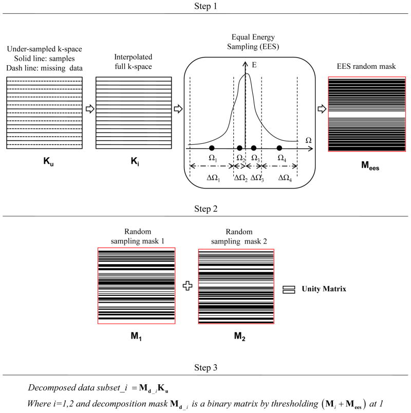
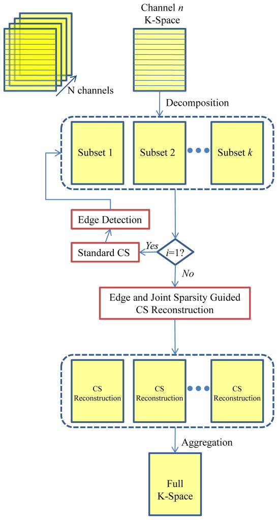
Starting with equidistantly under-sampled k-space data, we decomposed it into multiple sets of random k-space samples using the technique described in section 2.1, and then used both the standard CS and the edge guided CS with joint sparsity, which are explained in sections 2.2 and 2.3 respectively, to iteratively reconstruct full k-space data from each of the subsets. A flowchart depicting the proposed approach is shown in Fig. 1. CS reconstructions from different decompositions were averaged, giving a full calibration data for standard GRAPPA [12] to further remove artifacts and noise.

Fig. 1.

Flowchart of sampling decomposition method. Step 1 is to create the EES random sampling mask from the linearly interpolated k-space data. Step 2 is to create two random masks (N_d = 2). In step 3, the decomposition random masks are created from both EES mask and random mask and then used to decompose the original data set into two data subsets.

2.1. Sampling Decomposition

The motivation of random decomposition is to obtain measurements such that there exists an incoherence between the sampling matrix and the sparsifying matrices [2]. Given equidistant, variable-density, and under-sampled k-space data, multiple (N_d) sets of decomposition masks (M_d) were used to create decomposed data subsets. Both under-sampling and decomposing were performed along the same direction (e.g. phase encoding direction). A flowchart depicting the procedure to create M_d’s is shown in Fig. 1. An equipartition of the energy sampling (EES) scheme [20] was used to partition the spectral energy density of k-space data into a number of equal-energy sub-bands (denoted by ΔΩ in the figure) and then to create the EES random sampling mask (M_ees). Since the sampling scheme is about full Field-of-View (FOV), we chose full k-space linearly interpolated from undersampled data. Then, an M_d can be created by randomly selecting the phase encoding lines from M_ees, as explained in step 3 of the flowchart. We used the L₁-norm to calculate k-space energy [20]. For a 1D example in which the average energy of frequency encoded lines (denoted as E(Ω) where Ω ∈ [Ω_L, Ω_H ] is the frequency along phase encoding direction) and N acquired phase encodes are used, the i-th frequency value selected by EES scheme is

$$\left({\mathrm{\Omega }}_L+\sum _{k=1}^i\mathrm{\Delta }{\mathrm{\Omega }}_k-\frac{\mathrm{\Delta }{\mathrm{\Omega }}_i}{2}\right)\le {\mathrm{\Omega }}_i<\left({\mathrm{\Omega }}_L+\sum _{k=1}^i\mathrm{\Delta }{\mathrm{\Omega }}_k+\frac{\mathrm{\Delta }{\mathrm{\Omega }}_i}{2}\right)$$ (1)

with the width of the i-th subband

$$\mathrm{\Delta }{\mathrm{\Omega }}_i=\epsilon /\mid E\left({\mathrm{\Omega }}_i\right)\mid$$ (2)

where $\epsilon \equiv \frac{{\int }_{{\mathrm{\Omega }}_L}^{{\mathrm{\Omega }}_H}\mid E\left(\mathrm{\Omega }\right)\mid d\mathrm{\Omega }}{N}$ and Ω is the frequency along phase encoding direction.

This method creates variable density decomposition sampling mask which is based on the distribution of k-space signal energy, and we used it to decompose the k-space samples into N_d different subsets. Some high energy k-space signals were repeatedly assigned to every subset. Thus, each subset had a final sampling rate larger than 1/N_d, and a different M_d was customized for each different MR data set (due to its energy distribution).

2.2. The Standard CS Reconstruction

CS exploits the sparsity of an unknown image u to reconstruct it from many fewer linear measurements than required by the Nyquist-Shannon sampling theory. We used a standard CS basis pursuit reconstruction algorithm [2,3] to create the intermediate reconstructions that were then combined to form a high quality image.

In the context of application to MRI, the data y is obtained from partially sampling the Fourier transform of an image: y = F_pu + n = PFu + n, where P ∈ R^M×N is a selection matrix, and F is a Fourier transform matrix. In Ref.³, the unknown image u is solved from the following optimization problem:

$$\underset{u}{min}\alpha {\Vert \psi u\Vert }_1+\beta TV(u)+\frac{1}{2}{\Vert F_{p}u-y\Vert }_2^2$$ (3)

where ψ is a wavelet transform matrix; α and β control the contributions from ψ and total variation (TV) sparsifying transforms, respectively. For a two dimensional image u, isotropic discretization of TV(u) is ${\displaystyle \sum _{i,j}}\sqrt{{(u_{i+1,j}-u_{i,j})}^2+{(u_{i,j+1}-u_{ij})}^2}$ The success of solving Eq. (3) lies heavily on two tenets: the sparsity of u, and the incoherence between the sampling matrix F_p and the sparsifying matrix ψ.

2.3. Edge and Joint Sparsity Based CS Reconstruction

Starting with the intermediate reconstruction, we used edge detection and join sparsity to improve reconstruction. The intermediate reconstruction often included artifacts and noise, which can complicate edge detection. As a result, we used our previously published local mutual information (LMI) technique to separate real edges from fake ones [21]. We defined a binary mask matrix w that has value zero on edges and one elsewhere. A discretized weighted TV term was defined as: ${TV}_w(u)={\displaystyle \sum _{i,j}}{w}_{ij}\sqrt{{(u_{i+1,j}-u_{i,j})}^2+{(u_{i,j+1}-u_{ij})}^2}$ with w_ij = 0 if pixel (i,j) fell on edge and 1 elsewhere, was used to replace the TV term in Eq. (3). The same mask w was used across all channels, implementing joint sparsity across all channels. This joint sparsity forces reconstructions for each channel to share the same distribution of edges, which is reasonable since they are images of the same object. This new CS model was applied iteratively. A flowchart in Fig. 2 shows the procedure.

Fig. 2.

Flowchart of compressed sensing reconstruction.

The application of the new CS model to each decomposition of each channel results in a full k-space reconstruction of the image of interest, scaled by the corresponding coil sensitivity. First, within each channel, we aggregated reconstructions from different decompositions by averaging. A final, full field-of-view (FOV) image can then be formed by combining the different channels with a standard square root of sum of squares.

2.4. Standard and Proposed GRAPPA Reconstructions

In standard GRAPPA [12], the first step is to create the over-determined linear equations from the auto-calibrated signal (ACS) lines and estimate the complex coil weights by solving the equations with a least-squares algorithm. The coil weights are calibrated by fitting blocks of ACS signals from every coil to a single ACS line in one coil. We propose to modify this by using the CS reconstructed images to calibrate the GRAPPA kernel.

We call the proposed combined method for PPI image reconstruction “CS+GRAPPA”.

3. METHODS

We used both phantom and in vivo MR data sets to test the algorithms. To validate the effectiveness of decomposition, a Double-Stimulus Continuous Quality Scale (DSCQS) [15] observer experiment was used. We used a perceptual difference model (Case-PDM) [15] to objectively evaluate the CS+GRAPPA reconstructions due to the large number of images.

3.1. Data Description and Optimal CS Regularization Parameters

All data sets used for algorithm testing are described in Table 1. Datasets 1–2 were synthetic and real phantoms used for developmental testing of the decomposition method. We tested the CS+GRAPPA method on two sets of in vivo MR data (Datasets 3–4). All data were fully acquired in a Cartesian trajectory, and were synthetically under-sampled.

Table I.

Data descriptions

Data Name	Size (PExFExCoils)	Imaged Object	MR Scanner	Acquisition
Dataset 1	256×256×1	Shepp-Logan phantom	N/A	N/A
Dataset 2	256×256×8	Water phantom	Philips 3T Achieva	T2W TSE
Dataset 3	256×256×4	Volunteer’s brain	GE 1.5T Discovery	FLAIR
Dataset 4	198×256×8	Volunteer’s heart	GE 3T Discovert	GRE

α and β values in Eq. (3) were optimized by finding the lowest PDM score in an exhaustive search experiment on a wide range. Two optimal sets of α and β were used in the intermediate CS reconstructions. For the numerical phantom data set, we used empirically determined α and β values of order of 10⁻². For the MR water phantom and in vivo data sets, we used α and β values of order 10⁻⁵ and 10⁻², respectively.

3.2. Studying Decomposition Effectiveness and Artifact Reduction

We used Dataset 1, the numerical phantom, to evaluate how the proposed method reduced artifacts.

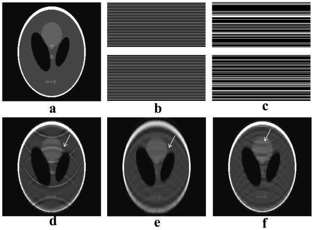
We compared the performance of CS reconstruction when applied to two different sampling schemes: equidistant, both with and without decomposition (Fig. 3b), and random under-sampling (Fig. 3c). Both had the same sampling rate, the same fully sampled central phase encoding lines, and the same total energy. The CS parameters (α and β) used here were optimal for both equidistant and random sampling schemes.

Fig. 3.

Effectiveness of decomposition in CS reconstruction. (a) is a reference image for the numerical phantom data. Two sampling schemes, equidistant scheme (b) and random scheme (c), have the same sampling rate (0.31), same fully sampled central phase encoding lines, and the same total energy. All CS reconstructions here share the same regularization parameters. Using standard CS with scheme (b), images (e) and (d) were reconstructed with and without decomposition, respectively. By visual inspection, the proposed decomposition method (N_d = 6) can significantly reduce aliasing artifacts. Image (f) was reconstructed from random scheme (c) by standard CS, showing some aliasing artifacts.

3.3. Selective Image Artifact Evaluation

We used artificial MR data in the human observer experiment for selective image artifact evaluation. Raw noisy data with mean Signal-to-Noise ratio (SNR) of 3.0, as measured in k-space, was simulated by adding Gaussian distributed noise independently to the real and imaginary channels of the k-space Shepp Logan phantom. It was then equidistantly under-sampled by different reduction factors to simulate different test data sets. These simulated data sets were decomposed into N_d data subsets and reconstructed with CS. To examine the effectiveness of the decomposition itself only, we used the standard CS model without edge detection. A final image was then obtained by aggregating these N_d CS reconstructions in k-space. A total 12 test images with a wide range of reconstruction qualities were created using sampling ratios of 0.54 and 0.31 and numbers of decomposition, N_d = 1–6.

To compare the performance of CS using decomposition with regard to individual types of artifacts, a Double-Stimulus Continuous-Quality Scale (DSCQS) experiment was employed [15], where noise, blur, aliasing, and overall image qualities were rated by human observers for test images created from Shepp Logan phantom. DSCQS is considered the most reliable method for subjective testing by the International Telecommunication Union of the television industry (Rec. ITU-R BT.500-10). These 12 test images were presented to the human observer in a random order, with each image displayed twice [15]. 6 engineering students were recruited for participating in this experiment. Image quality ratings from different subjects were averaged to reduce inter-subject variation if there was any. Further details about the DSCQS experiment can be found in Ref. [15].

3.4. Perceptual Difference Model (Case-PDM)

Since the reconstruction experiment generated thousands of test images using different parameters, we used a Perceptual Difference Model (Case-PDM) to objectively evaluate the image quality of reconstruction algorithms. PDM mimics human vision system to quantify the visual difference between the test and reference images. The reference image was the inverse Fourier transform of the full k-space data, while the test images were reconstructed from under-sampled k-space data by using GRAPPA and CS+GRAPPA. The output of PDM is a spatial map representing the magnitude of differences that a human observer would perceive between the input images [15]. This map can be summed over a region of interest (ROI) with relevant anatomy to give a scalar PDM score. In this paper, we chose the ROI to be the mask of the image. Zero score indicates the best image quality [15].

3.5. Comparing CS+GRAPPA to GRAPPA and 2-Step Iterative GRAPPA

We used Dataset 2, a water phantom, to evaluate the performance of the proposed method when applied to PPI. Standard GRAPPA [12], a 2-step iterative GRAPPA (i.e. coil calibration data is from full k-space of previous standard GRAPPA reconstruction) [30], and the proposed CS+GRAPPA reconstruction were used in this comparison study. Case-PDM was used to evaluate the images.

The performances of GRAPPA and CS+GRAPPA were further evaluated using two sets of in vivo data: Datasets 3 and 4 (i.e. one 4-channel brain data and 8-channel cardiac data). For both data sets, we used an N_d of 2, an α 10⁻⁵ and a β of 10⁻² in all intermediate CS reconstructions.

4. RESULTS

4.1. Single-channel Reconstructions

Comparison of Uniform and Random Sampling

When the standard CS model (Eq. 3) was directly applied to equidistantly under-sampled Cartesian k-space data, coherent aliasing artifacts were found, as expected (Fig. 3d). Random decomposition of equidistant measurements led to similar or reduced aliasing artifact, compared to the standard CS of random measurements (Fig. 3). This means that decomposition reduced aliasing artifacts at least as effectively as standard CS. However, blurring was introduced when 6 decompositions were used (Fig. 3e). More decompositions further decrease aliasing artifacts, at the expense of computational load and of blurring. These general observations were observed over a wide range of reduction factors and sampling patterns.

Subjective Evaluation of Artifacts

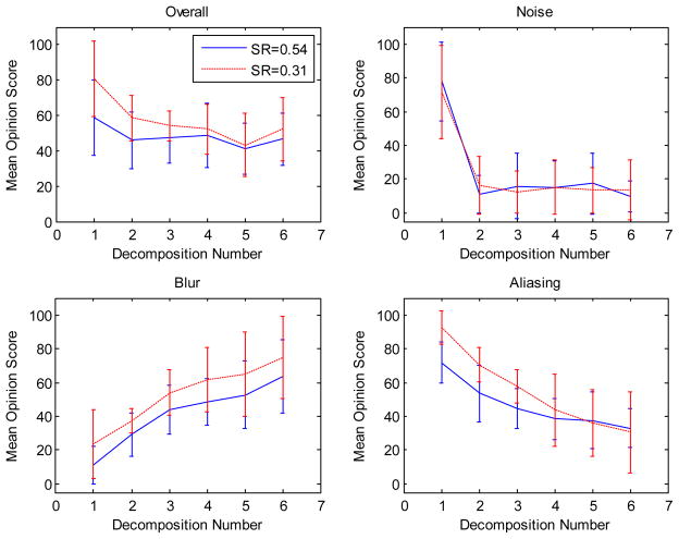
We next used a DSCQS human observer experiment to study selective-artifact-reduction performance of the decomposition method on CS reconstructions. Noise, blur, aliasing and overall quality ratings from different subjects were first averaged to give aggregate artifact-specific scores. Fig. 4 shows the subjective artifact ratings. The noise rating dropped to a stable value when two decompositions were used, suggesting that N_d = 2 is sufficient for noise reduction. When the number of decompositions N_d increased, aliasing ratings worsened, while blurring ratings consistently improved. The overall image quality improved when more decompositions were used.

Fig. 4.

Plots show summary of human subject ratings of overall, noise, blur, and aliasing image qualities, with 0 and 100 representing the best and the worst respectively, for test images generated by different sampling ratios (0.3 and 0.5) and decomposition numbers (N_d). The inter-subject standard deviations were calculated and are shown as error bars on the plots. When N_d increases, overall, noise and aliasing ratings improved, but blur ratings worsened.

4.2. PPI Reconstructions

Water Phantom Data

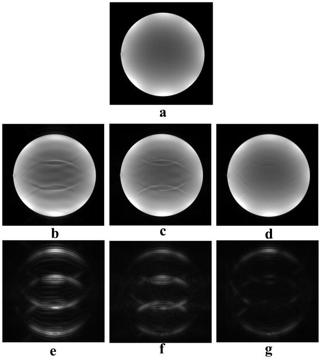
Using an 8-channel head coil, 3T MR water phantom data, we simulated a partial k-space parallel imaging acquisition using an outer reduction factor (or “ORF”, defined as reduction factor of data outside ACS) of 4, with 20 ACS lines. Standard GRAPPA, 2-step iterative GRAPPA, and the proposed CS+GRAPPA reconstruction were applied to the same data. The three GRAPPA reconstructions and their perceptual difference maps, along with the reference, are shown in Fig. 5. The edge and joint sparsity based CS model led to an almost artifact-free reconstruction, while standard GRAPPA reconstruction had significant aliasing artifacts. 2-step iterative GRAPPA also did little to reduce aliasing artifacts.

Fig. 5.

Images from different algorithms for 8-channel MR phantom data under-sampled by ORF=4 and ACS=20. The full k-space reference image (a) is compared to reconstructions from under-sampled data using GRAPPA (b), iterative GRAPPA (c), and CS+GRAPPA (d) with the edge and joint sparsity CS model. Images (e)-(g) are perceptual difference maps corresponding to reconstructions (b)-(d). CS+GRAPPA reconstruction has better image quality (PDM=0.77) than both GRAPPA (PDM=1.74) and iterative GRAPPA (PDM=1.34). Aliasing artifacts were almost completely removed by the proposed method, as determined by visually inspecting reconstructions (b) - (d) and their PDM maps.

In Vivo Data

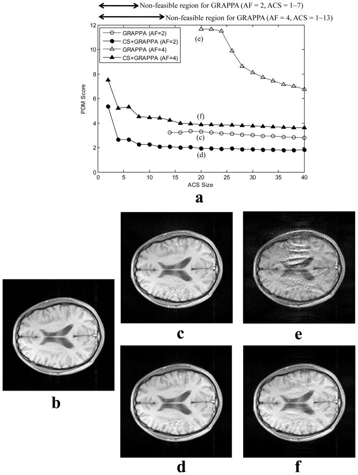
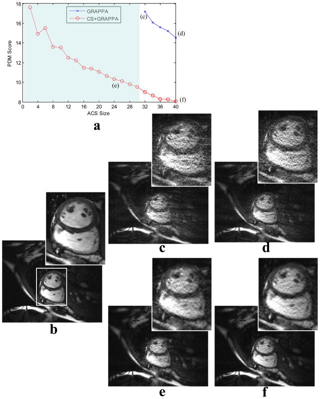
Figs. 6 and 7 show that CS+GRAPPA significantly improved image quality as compared to standard GRAPPA, as determined both by visual inspection and by PDM score. CS+GRAPPA significantly improved image quality of the brain data set, by an average of 1.7 times and 2.3 times for ORF’s of 2 and 4, respectively, and was able to generate reliable reconstructions with smaller ACS sizes than standard GRAPPA. Similar observations were obtained with a variety of data sets, with a variety of ORFs and ACS sizes.

Fig. 6.

Algorithm comparison for 4-channel brain data set. In plot (a), circles represent under-sampled data by ORF of 2 and triangles represent under-sampled data by ORF of 4. Open and solid marks represent standard GRAPPA and CS+GRAPPA (N_d=2) reconstructions, respectively. Plot (a) shows the relationship between image quality (in terms of PDM score) and different ACS size. CS+GRAPPA significantly improves the image quality (by an average of 1.7 times and 2.3 times for the ORF’s of 2 and 4), and is able to work with small ACS size, which is not feasible for the standard method. (b) is a reference image. At ORF=2 and ACS=20, image (c) was reconstructed by GRAPPA, and (d) was reconstructed by CS+GRAPPA. Noise is better removed by CS+GRAPPA. At ORF=4 and ACS=20, image (e) was reconstructed by GRAPPA, and image (f) was reconstructed by CS+GRAPPA. Both noise and aliasing artifacts are significantly more reduced by CS+GRAPPA. Image (f) has a comparable image quality to image (c). However, (f) was reconstructed by CS+GRAPPA from roughly half number of samples used by GRAPPA.

Fig. 7.

Algorithm demonstration for an 8-channel MR cardiac data set under-sampled by ORF=8. (a) plots the relationship between image quality (in terms of PDM score) and calibration data ACS size for both standard GRAPPA (marked by crosses) and CS+GRAPPA (marked by circles). (b) is a reference image. Letters (c–f) above marks in the plot correspond to images reconstructed either with different ACS sizes or by different methods. Zoom-in regions are also displayed together with the images. The edge and joint sparsity based CS model significantly improved GRAPPA reconstruction. Both noise and aliasing artifacts were significantly reduced as compared to the standard GRAPPA, even with use of less ACS data. The shaded area in the plot corresponds to non-feasible ACS sizes for the standard GRAPPA. However, CS+GRAPPA can work with much smaller ACS size.

As shown in Fig. 6, a comparable quality reconstruction can be achieved by CS+GRAPPA and GRAPPA. However, CS+GRAPPA needed almost half the number of samples and much less ACS data.

At an ORF of 4, an ACS size of less than or equal to 13 (i.e. 5.08% of full data with a total sampling rate of 28.8%) was not feasible for standard GRAPPA reconstruction. However, this small ACS size was not a problem for CS+GRAPPA, producing acceptable image quality for the brain data set even with ACS of 4 (i.e. 1.56% of full data with a total sampling rate of 26.2%). The cardiac data set showed similar patterns. CS+GRAPPA achieved an 81% average improvement in image quality over GRAPPA for the same sampling rate (Fig. 7).

5. DISCUSSION AND CONCLUSION

In this report, we have shown that Compressed Sensing reconstruction is possible and useful in fast MRI coherent acquisitions. Our CS+GRAPPA is able to accelerate GRAPPA imaging, achieving a quality GRAPPA reconstruction with both a higher reduction factor and less ACS data. The improvement of this method is the ability to use CS reconstructions for GRAPPA kernel calibrations by decomposing equidistant samples into multiple, random subsets. We found that this method can significantly reduce coherent aliasing and noise artifacts while enhancing image quality for regularly under-sampled MRI data. We found that two decompositions were sufficient to significantly reduce coherent aliasing and noise artifacts (Fig. 4). The advantage of decomposition is that it randomizes measurements in each subset, so that the incoherence between the sampling matrix and the sparsifying matrices is better satisfied. As a result, we were able to apply CS to an under-sampled equidistant data set and improve reconstruction quality. Numerical results in in vivo parallel MR data sets demonstrated that GRAPPA reconstruction can be significantly improved – PDM scores were halved on average with various sampling rates ranging from 7% to 40%. CS+GRAPPA allowed the same Case-PDM scores as standard GRAPPA, using about half the number of samples. The theoretical limit of GRAPPA is never approached because of limitations in artifacts [31]. Therefore, even though the theoretical minimum sampling rate is the same with CS+GRAPPA, it can actually be used for a faster and better PPI.

Using a standard CS algorithm, decompositions reduced coherent aliasing and noise artifacts at the expense of increased blurring. Due to the variable density sampling scheme, in which high power, lower frequency samples are more prevalent. CS reconstructions from these few samples cannot completely recover the missing high frequency samples, giving aggregated (average) k-space data with degraded content at high frequencies. To address the blurring issue, we used an edge and joint sparsity guided CS reconstruction, which was able to recover more accurate and sharp images with relatively few measurements [21,22]. This method differs from other image processing methods, such as low-pass filtering, which cannot eliminate aliasing artifacts.

The major computational load comes from the CS reconstructions for each decomposition and each coil. However, this computational load can be relieved both through parallel implementation of the algorithm and through use of an optimized CS algorithm. We compared a fast TVL1 CS algorithm [9] to a non-optimized TVL1 CS algorithm³. We found that the fast algorithm was about 4.6 times faster than the non-optimized algorithm when the codes were run on the same desktop PC (Dell Inspiron with Dual-Core Intel 3.5GHz CPU and 3G memory). GPU processing can further accelerate the CS computation a few hundred times [32]. Thus, with proper code optimization and implementation, we would not expect this extra load to hinder the application of the proposed method in the clinical environment.

There are several potential improvements with our algorithms. First, parameter tuning is an issue because of the sensitivity of CS algorithm. This issue can be solved with further research. The parameters α and β are directly related to noise level and sample size (Eq. 3). Noise level can be measured prior to the actual experiment or estimated using local variances etc., and sample size is known once the sampling pattern is determined. We can account for variations in parameters α and β by normalizing with respect to image size and sample size, after which the parameters could mainly depend on noise level. We need a future study to confirm this. Second, the effectiveness of the edge-based CS model relies on accuracy of edge mask matrix w obtained from standard CS model. More accurate edge detection methods from incomplete/noisy measurements will allow further reduction of aliasing artifacts by the decomposition method with better edge preservation and even less blurring. The LMI-based edge detection method proposed in section 2.3 does not work efficiently when there is still aliasing and noise in the image. A better method might be to detect edges directly from the under-sampled measurements (in k-space), instead of from the image reconstructed from the under-sampled measurements. Third, theoretical justification of the edge-based CS model has been completed if w_ij is set to be 0 when pixel (i,j) falls on edge. However, in practice, some preliminary experimental results show that a slightly better reconstruction can be obtained if a continuous scalar number between 0 and 1 is assigned to w_ij. As this needs further theoretical justification, we decided not to use it in our reconstructions. Last, a better way to aggregate CS reconstructions from different decompositions could further improve the result. We used a simple average. A better approach might be to maximize the conditional probability.

The idea of decomposition, edge and joint sparsity can all be easily applied to other CS models, for instance, the L_p (0<p<1) quasi-norm constrained model [10,26]. The proposed CS method can be easily adapted to other PPI techniques. For instance, it might be possible to estimate SENSE [11] coil sensitivity maps from intermediate CS reconstructions, which can then be used to unfold aliased image acquired by equidistant sampling. Thus, a SENSE reconstruction without needing pre-scan for coil sensitivity maps might be made possible. Our proposed CS+GRAPPA method might be especially suitable for dynamic MR imaging such as cardiac imaging in which all time frames share similar edge information of the same imaged object. In this case, reconstruction from the previous frame might be able to provide reliable edge information for reconstruction of the next frame.

References

- 1.Candes EJ, Romberg J, Tao J. Robust uncertainty principles: Exact signal reconstruction from highly incomplete frequency information. IEEE Trans Inf Theory. 2002;52 [Google Scholar]
- 2.Donoho DL. Compressed sensing. IEEE Trans Inf Theory. 2006;52:1289–1306. [Google Scholar]
- 3.Lustig M, Donoho D, Pauly JM. Sparse MRI: The application of compressed sensing for rapid MR imaging. Magn Reson Med. 2007;58:1182–1195. doi: 10.1002/mrm.21391. [DOI] [PubMed] [Google Scholar]
- 4.King KF, Marinelli L, Hardy CJ. Adaptive regularization in compressed sensing using the discrepancy principle. Proc. ISMRM; 2009. [Google Scholar]
- 5.Huang F, Chen Y, Yin W, Lin W, Ye X, Guo W, Reykowski A. A rapid and robust numerical algorithm for sensitivity encoding with sparsity constraints: self-feeding sparse SENSE. Magn Reson Med. 2010;64:1078–1088. doi: 10.1002/mrm.22504. [DOI] [PubMed] [Google Scholar]
- 6.Liu B, Sebert FM, Zhou Y, Yin L. SparseSENSE: Randomly-sampled parallel imaging using compressed sensing. Proc. ISMRM; 2008. [Google Scholar]
- 7.Beaty PJ, King KF, Marinelli L, Hardy CJ, Lustig M. Sequential application of parallel imaging and compressed sensing. Proc. ISMRM; 2009. [Google Scholar]
- 8.Lustig M, Pauly JM. SPIRiT: Iterative self-consistent parallel imaging reconstruction from arbitrary k-space. Magnetic Resonance in Medicine. 2010;64:457–471. doi: 10.1002/mrm.22428. [DOI] [PMC free article] [PubMed] [Google Scholar]
- 9.Yang J, Zhang Y, Yin W. Technical Report, TR08-27, CAAM. Rice University; A Fast TVL1-L2 Minimization Algorithm for Signal Reconstruction from Partial Fourier Data. [Google Scholar]
- 10.Chartrand Rick. Fast algorithm for nonconvex compressive sensing: MRI reconstruction from very few data. Proc. ISBI; 2008. [Google Scholar]
- 11.Pruessmann KP, Weiger M, Scheidegger MB, Boesiger P. SENSE: Sensitivity encoding for fast MRI. Magnetic Resonance in Medicine. 1999;42:952–962. [PubMed] [Google Scholar]
- 12.Griswold MA, Jakob PM, Heidemann RM, Nittka M, Jellus V, Wang JM, Kiefer B, Haase A. Generalized Autocalibrating Partially Parallel Acquisitions (GRAPPA) Magnetic Resonance in Medicine. 2002;47:1202–1210. doi: 10.1002/mrm.10171. [DOI] [PubMed] [Google Scholar]
- 13.Ji JX, Zhao C, Lang T. Compressed sensing parallel magnetic resonance imaging. Proc. of 30th Annual International IEEE EBMES Conference; Vancouver, British Columbia, Canada. August 20–24, 2008; [DOI] [PubMed] [Google Scholar]
- 14.Gamper U, Boesiger P, Kozerke S. Compressed sensing in dynamic MRI. Magnetic Resonance in Medicine. 2008;59(2):365–373. doi: 10.1002/mrm.21477. [DOI] [PubMed] [Google Scholar]
- 15.Miao J, Huo D, Wilson DL. Quantitative image quality evaluation of MR images using perceptual difference models. Medical Physics. 2008;35:2541–2553. doi: 10.1118/1.2903207. [DOI] [PMC free article] [PubMed] [Google Scholar]
- 16.Natarajan BK. Sparse approximate solutions to linear systems. SIAM Journal on Computing. 1995;24:227–234. [Google Scholar]
- 17.Donoho D, Elad M. Optimally sparse representation in general (nonorthogonal) dictionaries via l1 minimization. Proc. the National Academy of Sciences; 2003. pp. 2197–2202. [DOI] [PMC free article] [PubMed] [Google Scholar]
- 18.Donoho D, Huo X. Uncertainty principles and ideal atomic decompositions. IEEE Transactions on Information Theory. 2001;47:2845–2862. [Google Scholar]
- 19.Fuchs JJ. On sparse representations in arbitrary redundant bases. IEEE Transactions on Information Theory. 2004;50:1341–1344. [Google Scholar]
- 20.Suksmono AB. Compressive sampling with known spectral energy density. Proc. rICT; 2009. [Google Scholar]
- 21.Guo W, Huang F. In: Metaxas D, et al., editors. A Local Mutual Information Guided Denoising Technique and Its Application to Self-calibrated Partially Parallel Imaging; Proceedings of Medical Image Computing and Computer Assisted Intervention, 2008, Part II, Lecture notes on Computer Science; pp. 937–947. [DOI] [PubMed] [Google Scholar]
- 22.Guo W, Yin W. EdgeCS: Edge Guided Compressive Sensing Reconstruction. Proc SPIE Visual Communication and Image Processing. 2010;7744:77440L-1–77440L-10. [Google Scholar]
- 23.Daly S. The Visible Differences Predictor: An Algorithm for the Assessment of Image Fidelity. In: Watson AB, editor. Digital Images and Human Vision. MIT Press; Cambridge, MA: 1993. pp. 179–206. [Google Scholar]
- 24.Salem KA, Lewin JS, Aschoff AJ, Duerk JL, Wilson DL. Validation of a human vision model for image quality evaluation of fast interventional magnetic resonance imaging. Journal of Electronic Imaging. 2002;11:224–235. [Google Scholar]
- 25.Huo D, Wilson DL. Robust GRAPPA reconstruction and its evaluation with the perceptual difference model. Journal of Magnetic Resonance Imaging. 2008;27:1412–1420. doi: 10.1002/jmri.21352. [DOI] [PMC free article] [PubMed] [Google Scholar]
- 26.Trzasko J, Haider C, Manduca A. Practical nonconvex Compressive Sensing reconstruction of highly-accelerated 3D parallel MR angiograms. Proc. IEEE International Symposium on Biomedical Imaging; 2009. pp. 274–277. [Google Scholar]
- 27.Liang Zhi-Pei. Spatiotemporal imaging with partially separable functions. Proc. of the 4th IEEE International Symposium on Biomedical Imaging: From Nano to Macro, ISBI; 2007. [Google Scholar]
- 28.Liu B, King K, Steckner M, Xie J, Sheng J, Ying L. Regularized sensitivity encoding (SENSE) reconstruction using Bregman iterations. Magnetic Resonance in Medicine. 2009;61:145–152. doi: 10.1002/mrm.21799. [DOI] [PubMed] [Google Scholar]
- 29.Liang D, Liu B, Wang J, Ying L. Accelerating SENSE using compressed sensing. Magnetic Resonance in Medicine. 2009;62:1574–1584. doi: 10.1002/mrm.22161. [DOI] [PubMed] [Google Scholar]
- 30.Zhao T, Hu X. Iterative GRAPPA (iGRAPPA) for improved parallel imaging reconstruction. Magnetic Resonance in Medicine. 2008;59(4):903–907. doi: 10.1002/mrm.21370. [DOI] [PubMed] [Google Scholar]
- 31.Blaimer M, Breuer F, Mueller M, Heidemann RM, Griswold MA, Jacob PM. SMASH, SENSE, PILS, GRAPPA How to Choose the Optimal Method. Top Magn Reson Imaging. 2004;15:223–236. doi: 10.1097/01.rmr.0000136558.09801.dd. [DOI] [PubMed] [Google Scholar]
- 32.Jia X, Li R, Song WY, Jiang SB. GPU-base fast cone beam CT reconstruction from undersampled and noisy projection data via total variation. Medical Physics. 2010;37(4):1757–1760. doi: 10.1118/1.3371691. [DOI] [PubMed] [Google Scholar]