

Abstract
Quantitative evaluation of brain hemodynamics and metabolism, particularly the relationship between brain function and oxygen utilization, is important for understanding normal human brain operation as well as pathophysiology of neurological disorders. It can also be of great importance for evaluation of hypoxia within tumors of the brain and other organs. A fundamental discovery by Ogawa and co-workers of the BOLD (Blood Oxygenation Level Dependent) contrast opened a possibility to use this effect to study brain hemodynamic and metabolic properties by means of MRI measurements. Such measurements require developing theoretical models connecting MRI signal to brain structure and functioning and designing experimental techniques allowing MR measurements of salient features of theoretical models. In our review we discuss several such theoretical models and experimental methods for quantification brain hemodynamic and metabolic properties. Our review aims mostly at methods for measuring oxygen extraction fraction, OEF, based on measuring blood oxygenation level. Combining measurement of OEF with measurement of CBF allows evaluation of oxygen consumption, CMRO2. We first consider in detail magnetic properties of blood – magnetic susceptibility, MR relaxation and theoretical models of intravascular contribution to MR signal under different experimental conditions. Then, we describe a “through-space” effect – the influence of inhomogeneous magnetic fields, created in the extravascular space by intravascular deoxygenated blood, on the MR signal formation. Further we describe several experimental techniques taking advantage of these theoretical models. Some of these techniques - MR susceptometry, and T2-based quantification of oxygen OEF – utilize intravascular MR signal. Another technique – qBOLD – evaluates OEF by making use of through-space effects. In this review we targeted both scientists just entering the MR field and more experienced MR researchers interested in applying advanced BOLD-based techniques to study brain in health and disease.
Keywords: MRI, brain, BOLD, qBOLD, OEF, CMRO2, blood, susceptibility
1. Introduction
Quantitative evaluation of brain hemodynamics and metabolism, particularly the relationship between brain function and oxygen utilization, is important for understanding normal human brain operation (1) as well as understanding the pathophysiology of disorders such as stroke (2), Alzheimer’s disease (3–5), Huntington’s disease (6), Parkinson’s disease (7,8) and other neurological disorders (9–12). It can also be of great importance for evaluation of hypoxia within tumors of the brain and other organs (13,14). Currently, clinically accepted methods for measuring oxygen metabolism rely on PET techniques (e.g., (1)). However, the presence of ionizing radiation, low spatial resolution, and rather restricted availability inhibit broad application of PET-based methods in human research and clinical practice.
A fundamental discovery by Ogawa and co-workers (15) of the BOLD (Blood Oxygenation Level Dependent) contrast opened a possibility to use this effect to study brain hemodynamic properties by means of MRI measurements. The most widely used application of BOLD contrast is based on studying dynamic properties of brain during functional stimulation, i.e. fMRI (functional MRI) (16–19). However, BOLD effect can also be used to studying brain hemodynamic in a resting (baseline) state because, despite heterogeneities in blood flow and metabolism amongst brain regions, a long-standing observation is that in healthy human subjects oxygen extraction fraction (OEF), on average, is remarkably constant across the brain in the resting state (20) and can be used as the primary index of brain function (20,21). This baseline state is usually achieved with the subject resting quietly but awake with eyes closed. Such a baseline state can be described as a default mode of the brain activity. Therefore, it is important to understand the quantitative characteristics describing this default mode. In this regard, it should also be noted that it is the baseline functional activity of the brain that is responsible for the majority of the brain’s enormous energy budget (1).
Regional OEF measurements can assess compensatory responses made by the brain to progressive reductions in cerebral perfusion pressure (CPP) (e.g., (22,23)). When CPP is normal, CBF is closely matched to the resting metabolic rate of the tissue. As a consequence of this resting balance between flow and metabolism, the OEF shows little regional variation. Moderate reductions in CPP have little effect on CBF, as vasodilation of arterioles reduces cerebrovascular resistance, thus maintaining a constant CBF. With more severe reductions in CPP, the capacity for compensatory vasodilation is exceeded and CBF begins to decline. Cerebral oxygen metabolism and brain function at this stage are maintained by progressive increase in OEF (2,24). Importantly, the OEF has been shown to be an accurate predictor of subsequent stroke occurrence in patients with cerebrovascular disease (25,26) supporting the idea that OEF is a critical hemodynamic parameter that provides an important and predictive index of brain functional status.
Combining OEF measurements with measurements of cerebral blood flow (CBF) enables the evaluation of cerebral metabolic rate of oxygen consumption (CMRO2) by means of Fick’s principle. Different methods of CBF quantification will be discussed in other papers of this special issue of NMR in Biomedicine. In this article we focus our attention on MRI-based methods for measuring OEF. Our review is targeted to both scientists just entering the MR field and more experienced MR researchers interested in applying advanced BOLD-based techniques to study brain in health and disease.
2. Fick’s principle
According to Fick’s principle (27), CMRO2 can be calculated by using the following relationship:
| [1] |
where Ya and Yv are oxygenation levels of arterial and venous blood (i.e., the fraction of hemoglobin in the form of oxyHb; Y = 1 corresponds to fully oxygenated blood and Y = 0 corresponds to fully deoxygenated blood); and Cblood is blood oxygen carrying capacity. Usually, CMRO2 is measured in μmol O2/g tissue/min, CBF in ml blood/g tissue/min, and Cblood in μmol O2/ml blood.
Strictly speaking, Eq. [1] corresponds to oxygen combined with hemoglobin, ignoring oxygen dissolved in blood plasma. The amount of dissolved oxygen is determined by partial pressure of oxygen PO2 in blood (28):
| [2] |
and usually does not exceed 1.5% of total oxygen in blood though it can be higher in abnormal conditions, e.g. hyperoxia (29).
The hemoglobin-based blood oxygen carrying capacity is proportional to blood hematocrit level Hct:
| [3] |
where the proportionality coefficient CRBC is oxygen carrying capacity of red blood cells (RBC). Hence, Eq. [1] can be written as follows:
| [4] |
where oxygen extraction fraction is defined as
| [5] |
Oxygen carrying capacity CRBC can be calculated as
| [6] |
where nHb = 5.5 · 10−6 mol/ml is the concentration of hemoglobin in RBC (30), MHb = 64,450g/mol is the hemoglobin molecular weight (31), and CHb = 1.39 ml/g is amount of oxygen that can be combined with 1g of pure hemoglobin (28). Thus, CRBC = 0.493 (ml O2/ml RBC).
According to Eqs. [1], [4], if CBF and OEF are known, oxygen consumption CMRO2 can be calculated. Several reviews in the current issue of this journal are devoted to methods of measuring CBF. Our review aims mostly at methods for measuring OEF. Most of the current MR methods of measuring OEF are based, in fact, on measuring blood oxygenation level. Some of these methods and theoretical backgrounds behind these methods are discussed in the present review.
3. Blood Oxygenation and MR Signal
One of the important parameters characterizing magnetic properties of all tissues is their magnetic susceptibility χ – a proportionality coefficient between tissue magnetization, M, induced by an external magnetic field B0, and the magnetic field strength (note that we are using Gaussian-CGS units throughout):
| [7] |
Most components of biological tissues, such as water, proteins, lipids, are diamagnetic (their magnetic susceptibility χ is negative). The diamagnetism is a common property of all atoms and molecules; it is due to the effect of changing microscopic atomic currents of orbiting electrons, sometimes called Ampèrian currents, in the presence of magnetic field B0. If atoms or molecules contain uncompensated electronic spin moments (that is always accompanied by magnetic moment), they also exhibit additional magnetic susceptibility which is positive and is called paramagnetic susceptibility. The paramagnetic effect is due to “orientational nature” of magnetic field that tends to align electron spin magnetic moments against “de-orientational nature” of thermal motion. Paramagnetic susceptibility is described by the Curie law:
| [8] |
where N is a molar content of paramagnetic molecules per unit volume, μ - their molecular spin-based magnetic moment, kB – Boltzmann constant and T – absolute temperature. Biologically relevant examples of paramagnetic molecules include non-heme iron and heme iron in deoxyhemoglobin (see detail discussion in (32–34)), and dissolved oxygen molecule O2. Importantly, heme iron is paramagnetic because of its Fe2+ state. When heme iron combines with oxygen, it changes its electronic configuration and the total spin magnetic moment of heme complex becomes zero (35,36). When heme iron releases oxygen, it returns to a paramagnetic state. Hence, magnetic state of heme iron can be used as a biomarker of blood oxygenation level. When blood passes through the capillary bed and releases oxygen, the state of heme iron changes from zero-spin at the arterial side to a high spin at the venous side.
Due to these reversible changes of heme complexes in deoxygenated red blood cells (RBC) (35,36), the blood vessel network in biological tissues modifies MR signal. Importantly, this modification depends on blood oxygenation level. This phenomenon forms the basis of the BOLD (blood oxygen level dependent) contrast in MRI. Two effects should be separated – intravascular and extravascular. The intravascular effect is due to the inhomogeneous magnetic fields created by red blood cells in blood (37). The extravascular (through-space) effect is mainly due to inhomogeneous magnetic fields created by blood vessels in the surrounding tissue (15,38). Because these magnetic field inhomogeneities are tissue specific, they can provide important information on tissue hemodynamic properties. To quantify these changes, MRI techniques based on Free Induction Decay (FID) and different versions of spin echo (SE), including multi-SE sequences, such as CPMG and its variations (e.g. (39)), are usually used. In these experiments, the MR signal S(t) can be described in terms of a signal attenuation function Γ(t):
| [9] |
where t is either time after initial excitation RF pulse in FID and CPMG experiments or spin echo time in SE experiment. It is usually assumed that
| [10] |
where R2 and are irreversible and reversible (with respect to 180° refocusing RF pulse) MR signal relaxation rate constants and ϕ(t) is the MR signal phase contributed by tissue specific sources and also by unwanted macroscopic field inhomogeneities. Note that in multi-SE experiments, R2 depends on inter-echo spacing, R2 = R2(τCPMG), e.g. (40,41).
In fact, Eqs. [10] are rarely accurate in biological tissues because the signal attenuation function Γ(t) is a non-linear function of its argument and depends on the type of MR experiment. An obvious source of non-linearity of the signal attenuation function relates to a multi-compartment tissue structure. Another source of the deviation from simple exponential decay (even for a single compartment case) relates to the presence of inhomogeneous magnetic fields (42–58). This type of non-linearity will also be discussed in detail in this review paper.
4. Intravascular MR Signal
4.1 Blood magnetic susceptibility
Studies of the magnetic properties of human blood have been undertaken in numerous publications (35–37,57,59–78). A detailed theoretical consideration of blood magnetic susceptibility and the detailed experimental studies employing in vitro samples that were well representative of human blood in situ were provided in (71). Here we briefly outline these results. The magnetic susceptibility of whole blood is determined by a weighted sum of magnetic susceptibilities of RBC and plasma:
| [11] |
where Hct is the blood hematocrit level.
The magnetic susceptibility of RBC can be expressed as (71):
| [12] |
where Y is blood oxygenation level, χg,prot = −0.587 · 10−6 mL/g is diamagnetic contribution of the Hb protein (79), νM,Hb = 48,277 mL/mol is the molar volume of Hb in solution (79), and the rest of the parameters are defined in Section 2. The paramagnetic contribution to the molar susceptibility of deoxyHb, χM,dHb, can be calculated via Eq. [8]. Taking into account that there are 4 iron atoms per heme complex, and that the average magnetic moment of Fe2+ in hemoglobin, μ = 5.46μB/Heme (μB is the Bohr magneton) (36), it can be calculated that at 37°C, χM,dHb = 48.082 · 10−6 mL/mol. Thus, the magnetic susceptibility of RBCs can be described as (71):
| [13] |
Susceptibility of plasma, χplasma, can be estimated based on the contributions of water and the other major plasma constituents (proteins), which accounts for approximately 93% and 7% of the plasma weight, respectively (80). As a result, χplasma is slightly different from susceptibility of water, χH20 = −0.719ppm (71),
| [14] |
Thus, the total susceptibility of whole blood is
| [15] |
Important prediction of this equation is that the susceptibility difference between completely deoxygenated (Y = 0) and completely oxygenated (Y = 1) RBC is equal to
| [16] |
Equation [16] was confirmed by two independent MR and SQUID magnetometer measuremerecently by detail magnetic susceptometry measurements (77). A rather close value was also reported in (81). Note that the value Δχ0 = 0.27ppm in Eq. [16] is substantially (50%) larger than that frequently used (Δχ0 = 0.18ppm) - for historical reasons - in the MRI literature.
Magnetic susceptibility of oxygen dissolved in blood plasma, χ[O2], can be readily calculated based on the Curie law, Eq. [8]:
| [17] |
where Na is Avogadro’s number, V0 is gas molar volume at normal conditions, and μeff = 2.83 · μB per 1 molecule of oxygen. Using Eq. [2] for dissolved oxygen concentration in blood, we get
| [18] |
This quantity is rather small as compared to the paramagnetic component of the magnetic susceptibility of deoxyHb. For example, at PO2 = 100 mmHg, the contribution of oxygen to blood magnetic susceptibility is χ[O2] = 0.00039 ppm, while at Hct = 0.4 and blood oxygenation level Y=0.6, the contribution of the paramagnetic component of the magnetic susceptibility of deoxyHb to the blood magnetic susceptibility is ΔχdeoxyHb = 0.0432ppm - two orders of magnitude higher. In what follows, the contribution of dissolved oxygen to blood magnetic susceptibility will be ignored.
Equation [15] determines the susceptibility of the whole blood. For the purpose of study of OEF and CMRO2 in the brain, one should refer χblood to the magnetic susceptibility of surrounding tissue:
| [19] |
The tissue susceptibility χtissue is determined by a variety of susceptibility inclusions: first of all, proteins, lipids, and non-heme iron. For example, based on cellular content and related physical properties of the essential inclusions in an “average normal” frontal lobe cortical GM, WM and CSF/ISF, the volume magnetic susceptibilities of the inclusions (relative to water) were estimated in (82) and provided here in Table 1. Thus, the magnetic susceptibility difference between blood and surrounding tissue can be calculated as follows:
| [20] |
where Δχtissue = χtissue − χH2O in ppm (see Table 1). This means that the susceptibility difference between blood and surrounding tissue is not zero even for fully oxygenated blood. Hence, the blood oxygenation level can be determined from the experimentally measured Δχ as follows:
| [21] |
Table 1.
The susceptibility of “average normal” tissue (relative to water, excluding intravascular blood) in frontal lobe (in 10−3 ppm) (82)
| GM | WM | CSF | |
|---|---|---|---|
| Proteins | −4.17 | −4.56 | −0.0016 |
| Lipids | 2.37 | 5.52 | 0 |
| Non-heme iron | 4.40 | 4.40 | 0.33 |
|
| |||
| Total | 2.6 | 5.36 | 0.33 |
For arterial and venous blood, Y = Ya and Y = Yv, respectively. OEF can be calculated from these parameters using Eq. [5]. Note that a usually used relationship
| [22] |
where Δχ0 is given in Eq. [16], is an approximation of Eq. [20] that neglects differences between magnetic susceptibilities of tissue, water and plasma.
4.2 MR signal from blood vessel network
The susceptibility difference between blood (χblood) and tissue (χtissue) results in difference of the Larmor frequency of protons in water molecules within blood vessels and those in surrounding tissue, Δω. Approximating a blood vessel by a long circular cylinder, Δω can be written as (83)
| [23] |
where θ is the angle between the vessel direction and the direction of magnetic field B0. The term 1/3 in Eq. [23] reflects a contribution of the so called Lorentzian sphere (e.g., (84)). One should however note that the Lorentzian sphere approximation might not be adequate for describing influence of tissue microstructure on MR frequency. To accurately predict the Larmor resonance frequency difference between intravascular and extravascular water protons in tissues with long cells (i.e. axons), the generalized Lorentzian theory (82) should be used. However, since susceptibilities of GM and WM tissues (see Table 1) are much smaller than that of venous blood, the influence of this effect on Eq. [23] might be small.
The normalized MR free induction decay (FID) signal from a single vessel with the frequency shift Δω is described as a simple exponential oscillation, s1(t) = exp(−i · Δω · t), (transverse relaxation of blood signal will be introduced later). However, each imaging voxel contains blood vessels with different orientations, and the total MR signal form a voxel is a sum of the signals from individual vessels:
| [24] |
where P(θ) is the distribution function of vessel orientations. This distribution is usually not isotropic (85), however for low resolution experiments when an imaging voxel contains a multitude of blood vessels, a uniform distribution, P(θ) = sin θ/2, can be a reasonable approximation. In this case the signal si(t) can be readily calculated (52) (see also (86)):
| [25] |
where Δω0 = 2πγ B0 Δχ, and C(·) and S(·) are the Fresnel functions (note that we use here the definition of the Fresnel functions as in (87) which is different by the factor π/2 in the argument from that used in (88) and adopted in (86)).
Equation [25] describes contribution to MR signal of blood with a given oxygenation level. However, blood oxygenation is different between arteries, capillaries and veins. To address this issue, Eq. [25] can be modified by introducing a distribution function of characteristic frequencies, Δω0. This is not difficult to incorporate into theoretical model but accounting for this effect in experiments might be a challenge.
4.3 Blood transverse relaxation – T2 and
The signal decay described by Eq. [25] does not take into account intrinsic T2 (or ) MR relaxation processes in blood, usually described phenomenologically by R2 (or ) relaxation rate constants for SE and FID signals correspondingly. The presence of inhomogeneous magnetic fields created in the blood by deoxyHb, increases R2 and relaxation rate constants (37). Generally, these transverse relaxation rate constants of blood can be presented as
| [26] |
where the first terms correspond to the case when magnetic susceptibilities of RBCs and plasma are identical. According to Eqs. [13]–[14], it takes place at 1 − Y = 0.05 (71) (see Eq. [27] below). In this case there is no frequency shift between RBC and plasma, and one would expect that should be the same as R20. This was indeed observed at 1.5T measurements in (71,74) but not at 4.7T (74). An explanation of this effect is still pending. Experimental values for R20 and found for human and bovine blood at 1.5T (e.g., (71,74,81,89)), vary in the interval 4–7 s−1. The second terms in Eqs. [26] describe the contribution of water diffusion in the inhomogeneous magnetic field induced by the magnetic susceptibility difference between RBC and plasma,
| [27] |
Description of MR signal in terms of R2 and/or relaxation rate constants assumes that the signal decay can be described by a simple exponential. In fact, experimental data in (71) demonstrated a substantial deviation from such a behavior, hence MR signal should be described in general terms of a non-linear signal attenuation function Γ(t) in Eq. [9]. Specifically, for a realistic model of blood this function was calculated in (72) using previously developed Gaussian-phase-approximation-based approach (53).
It was demonstrated that for an arbitrary shape of susceptibility inclusions (in our case, RBC), at short time, t ≪ tD (tD is a characteristic diffusion time, see below), ΓFID(t) ~ t2 for FID signal and ΓSE(t) ~ t5/2 for single spin-echo (SE) pulse sequence. The asymptotic behavior of ΓFID(t) and ΓSE(t) at long time, t ≫ tD, is as follows
| [28] |
where
| [29] |
Deff = DRBC · Hct + Dplasma · (1 − Hct) is the effective water diffusion coefficient (DRBC and Dplasma are water diffusion coefficient in RBC’s cytoplasm and blood plasma, respectively); tp = 4π/3 · γ · Δχp · B0−1 is characteristic dephasing time; the double integration in [29] is over the volume of a single RBC v. The coefficients aFID and aSE in Eq. [28] are RBC shape-specific numerical coefficients. For a spherical shape they are 0.89 and 1.6 for FID and SE experiments, respectively.
Figure 1 illustrates a typical time dependence of the signal attenuation functions ΓFID(t) and ΓSE(t) normalized to the characteristic value Γ0,
Figure 1.

Time dependence of the signal attenuation functions ΓFID(t) and ΓSE(t) (normalized to the characteristic value Γ0, Eq. [30]) calculated in the Gaussian phase approximation (adapted from (53)).
| [30] |
In (72), the shape of RBC was modeled as a biconcave disk which can be obtained by rotating the curve given in Eq. [31] about the ordinate z (90):
| [31] |
The curve z (x) is depicted in Figure 2. For the normal human RBC, c0 = 0.188, c1 = 1.085, c2 = −0.896, lRBC = 3.825μm, and the RBC volume v = 97.91μm3 (90). For these specific RBC parameters, a numerical evaluation of the integral divided by v in Eq. [29] gives . Using Eq. [27], the quantity ΔR2 can be written in the form:
| [32] |
where and τ0 = 4π/3 · γ · Δχ0 · B0−1 are the characteristic diffusion and dephasing times (the numerical coefficient in Eq. [32] differs from that in (72) due to different definition of the characteristic times τ0 and tD).
Figure 2.
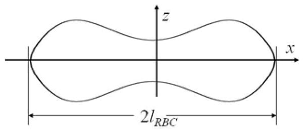
The RBC shape described by Eq. [31].
It should be noted that the Gaussian phase approximation is valid under assumption that the characteristic diffusion time is less than the characteristic dephasing time, λ = tD/τ0 ≪ 1. For typical value of the average water diffusion coefficient Deff = 2μm2/ms, we get for B0 = 1.5T, 3 T and 4.7 T: λ = 0.22, 0.44 and 0.69, respectively. Consequently, one can expect that our approach should be accurate for B0 = 1.5T and 3T but might not be accurate for B0 = 4.7T. Indeed, for B0 = 1.5T, Eq. [32] gives κ = 51.8sec−1 which is in a good agreement with value κ = 55sec−1 obtained experimentally in (71). Detail results of measurements at different field strength can be found in (71,74,81,91) for different types of MR experiments.
A semi-phenomenological theory of FID signal relaxation in blood was proposed in (57). In this approach blood is considered as a heterogeneous media characterized by a correlation length lc. In case of a small variation of the Larmor frequency (characterized by the dispersion δΩ), the FID signal is described as follows (57):
| [33] |
where α = δΩ · τD, τD = (lc/2π)2/D is the characteristic diffusion time, D is the diffusion coefficient (assumed to be the same for RBC and plasma). The expression [33] differs from a standard bi-exponential function broadly used in MR literature by a negative sign in the pre-exponential factor in the first term. As demonstrated in (57), the fit of Eq. [33] to experimental data provides a reasonable agreement between the value δΩfit = 0.86ms−1 and the experimental δΩ = 0.69 ms−1.
The previous discussion addressed blood relaxation properties for FID and SE experiments. For a CPMG sequence, when RF excitation pulse follows by a train of 180° refocusing pulses, blood properties were discussed in (37,81,89,92,93) in the frameworks of different models. In the two-compartment Luz-Meiboom exchange model (41), the quantity ΔR2 in Eq. [26] for CPMG pulse sequence is equal to (81,89),
| [34] |
where τexch is the phenomenological parameter describing the exchange lifetime, τCPMG is the inter-echo spacing. Equation [34] assumes that the two compartments (RBC and plasma) have a characteristic susceptibility-induced Larmor frequency shift Δω.
The expression for ΔR2 [34] is valid in the limit of fast exchange, Δω · τexch ≪ 1, and at short inter-echo spacing, Δω · τCPMG < 2 (see discussion in (93)). A more complex exchange model valid in the slow-exchange regime (Δω · τexch > 1) and for long echo spacing (Δω · τCPMG > 2) was developed in (94,95). In this model, the quantity ΔR2 is
| [35] |
Equations [34] and [35] are based on the models that treat diffusion of water molecules in blood as a two-cite exchange process. Another approach to account for diffusion in CPMG experiment was proposed by Jensen and Chandra (50) in the framework of the so called weak field approximation. With an additional assumption that the Larmor frequency correlation function monoexponentially decreases with time, they found the same functional form for ΔR2 as in Eq. [34]. However, as demonstrated in the same study (50) for the model of magnetized spheres the frequency correlation function decreases with time in an algebraic way (see also (53,54)). In this case, the quantity ΔR2 for a CPMG pulse sequence was found to be (50):
| [36] |
As we discussed above, a general time dependence of MR signal attenuation function Γ(t) in the FID and SE experiments is nonlinear. The same might take place for the CPMG experiment, though the CPMG sequence have a tendency to “restore” the linear time dependence of Γ(t) as a function of spin echo number (t = tn) in the CPMG echo train. Such a “restoration” was exemplified in the original paper by Carr & Purcell (40), by considering diffusion in a constant magnetic field gradient (see also discussion in of this issue in (96)). Though we should note that the dependence of ΔR2 on the echo spacing, τCPMG, still remains non-linear. A detail discussion of this behavior is beyond the scope of this paper.
5. Theoretical models of Extravascular MR Signal
In the previous section we discussed the intravascular contribution to MR signal attenuation from blood vessel network. The total MR signal includes also the signal from surrounding tissue where inhomogeneous magnetic field is induced due to the susceptibility difference Δχ between blood containing paramagnetic deoxyHb and tissue, Eq. [20]. Thus, spins of water protons in the extravascular space sustain different phase shift ϕ, leading to additional MR signal decay. The signal at time t after excitation is given by the average of the contributions from all the spins across the volume
| [37] |
where ϕ(t) is the phase accumulated by a single spin by time t, and <…> means averaging over all possible initial positions and trajectories of a spin. In an inhomogeneous magnetic field, h = h(r), the phase ϕ(t) of the spin moving along a given trajectory r = r(t) can be written as
| [38] |
Inhomogeneous magnetic field h(r) is created by a multitude of blood vessels with different positions and orientations. As magnetic field obeys linear superposition, a spin’s phase can be found by integrating the sum of frequency shifts Δωn(t) caused by each of N vessels:
| [39] |
For a single blood vessel of cylindrical shape, the local Larmor frequency shift Δω(r) in tissue is given by a well known expression (e.g., (83)):
| [40] |
Several theoretical approaches have been proposed to calculate MR signal in Eqs. [37]–[40] (e.g., (42,44–50,52–54,97)). A Monte-Carlo-based analysis was also used for this purposes (e.g. (55,67,83,98–100)). Herein we will discuss in detail the static dephasing model (42), the models based on a Gaussian phase approximation (44,53,54) and a phenomenological model (100). Two other approaches – the so called weak and strong field approximations – were proposed in (49,50). The so called “strong collision approximation” was introduced in (47,48). The model proposed in (45) exploits the “linear local field approximation”, in which spins are considered to diffuse in a local (constant for each spin) field gradient. A validity analysis of some of these models was conducted in (100). Some of these results will also be presented here.
5.1 Static dephasing regime
An exact analytical expression for the FID signal was first derived in (42) in the important case of a static dephasing regime when the characteristic dephasing time of MR signal decay in the presence of inhomogeneous magnetic fields is smaller than the characteristic diffusion time (see details below). As shown in (42), in the case of blood vessels with a uniform distribution of their orientations, the extravascular FID signal in the presence of magnetic field inhomogeneities induced by blood vessel network can be presented in the form of Eq. [9] with
| [41] |
where zero time t corresponds to the position of RF excitation pulse, R2 = 1/T2 describes a T2-relaxation in tissue, ζ is the deoxyhemoglobin-containing part of cerebral blood volume (dCBV) - veins and pre-venous part of capillaries. Strictly speaking, the presence of blood vessel network in the tissue also creates frequency shift in Eq. [41] that depends on details of tissue structure at both cellular and global levels (82). The characteristic dephasing time is determined as:
| [42] |
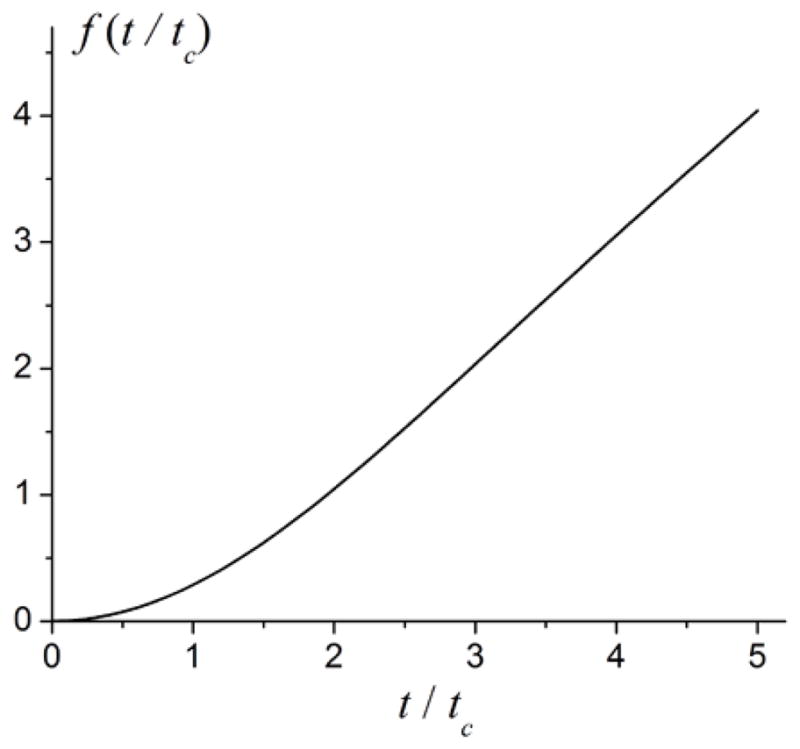
The function f(t/tc) in Eq. [41] is given by (42)
| [43] |
where J0 is a Bessel function. The function f(t/tc) can also be represented using a generalized hypergeometric function 1F2 (52):
| [44] |
Comments about the parameter ζ = dCBV are in order as it is sometimes confused with CBV - a parameter defined by other techniques, such as PET, which measure the total blood volume. Only blood that has magnetic susceptibility different from the magnetic susceptibility of brain parenchyma contributes to field inhomogeneities that lead to tissue water MR signal decay described in Eqs. [41]–[44]. Recall, that the major contribution to this magnetic susceptibility difference is due to the presence of deoxyhemoglobin in blood, Eq. [20]. This deoxyhemoglobin containing blood constitutes only part of the blood vessel network, namely, the venous blood vessel network and part of the capillary network adjacent to venous side (capillary blood becomes deoxygenated as it moves from arterial to venous side). According to Eq. [20], there is a non-zero magnetic susceptibility difference even between the completely oxygenated blood in arteries (Y = 1) and surrounding brain parenchyma. However, this difference is rather small and usually can be neglected. In order to avoid confusion, we will call the parameter ζ the deoxygenated Cerebral Blood Volume (dCBV).
The function f(t/tc) in Eq. [44] is illustrated in Figure 3. In the short-time and long-time regimes, the function f(t/tc) depends on its argument quadratically and linearly, respectively:
| [45] |
Figure 3.
The linear behavior of the function f(t/tc) at large argument leads to a linear behavior of the signal attenuation function:
| [46] |
Importantly, the volume fraction ζ and the susceptibility difference Δχ appear in Eq. [46] only as a product, hence to resolve these two parameters, measurement interval should include short time regime t < tc (43) where parameters ζ and Δχ decouple because the function f(t/tc) exhibits a quadratic time dependence, Eq. [45].
Since the short time interval is important for decoupling of parameters ζ and Δχ, it was proposed in (43) to use GESSE (gradient echo sampling of spin echo) approach (see Figure 4b) when MR signal is sampled around spin echo (SE). This strategy practically doubles the short time interval as compared to the FID experiment. The expression for MR signal around SE (GESSE signal) is given by Eq. [9] with
Figure 4.

Time dependence of the simulated FID (A) and GESSE (B) signals at different vessel radii R. Input parameters are: OEF = 0.4, ζ = 0.03. Light blue lines correspond to the case D = 0 (static dephasing regime – SDR). All other lines correspond to D = 1μm2/ms. Spin echo time TE = 60ms corresponds to t = 0 in (B) (shown by dashed vertical line). The transverse T2 relaxation is ignored. (Modified from (100)).
| [47] |
where time t is counted from spin echo time TE (and can be negative, though t >−TE/2).
It is important to note that the results in Eqs. [41] and [47] depend only on the total volume of blood vessels with the partially deoxygenated blood and does not depend on specific distribution of blood vessels. This result is in a very good agreement with the results obtained by others by means of Monte-Carlo computer simulations (83) and (98). This very important theoretical prediction allows application of this theory (42) to in vivo studies where a rather broad microscopic distribution of blood vessels can be expected.
Equations [41] and [47] were derived in the static dephasing regime framework. Here the presence of susceptibility-induced static magnetic field inhomogeneities cause the MR FID signal to decay much faster than a competing process, the averaging of the water 1H nuclear spin phases due to molecular diffusion. Validity criteria of the static dephasing regime analysis have been discussed in detail in (42,43). According to (42), the static dephasing regime for the FID signal holds if the characteristic dephasing time tc, Eq. [42], is smaller than the characteristic diffusion time, tD = R2/D, where D is the water diffusion coefficient (in the brain, D ~ 1μm2/ms) and R is the characteristic blood vessel radius. For the blood vessel network modeled by randomly oriented cylinders discussed above, this condition is
| [48] |
The inequality [48] puts a restriction on the blood vessel radii, R, for which the static dephasing regime is valid:
| [49] |
For B0 = 3T, γ = 2.675 · 108 sec−1T−1, Δχ = 0.04ppm (for venous blood with the Hct=0.4 and Y=0.6), the characteristic dephasing time tc = 7.4 ms, and the inequality [49] results in R > 6μm. Thus, for the FID signal, the static dephasing regime might not quantitatively describe MR signal behavior in the presence of capillaries but is a very good approximation for the post-capillary blood vessel network (venules, veins, etc.).
The effect of water diffusion and validity criteria of the static dephasing regime were discussed in a number of publications, e.g. (42,43,46,53,54,100–102). Some of these approaches will be discussed in detail below.
5.2 Gaussian Phase Approximation (role of water diffusion)
To describe the MR signal attenuation for small capillaries, the Gaussian phase approximation can be used (53,54). In the framework of this approach, the expression for the signal, Eq. [37], is presented in the form first proposed in (103):
| [50] |
where P(ϕ) is a phase distribution function. As shown in (103), in the case of unrestricted diffusion in the constant field gradient, this function is of the Gaussian type:
| [51] |
and the MR signal corresponding to P ϕ, t in Eq. [50] can be described by Eq. [9] with signal attenuation function
| [52] |
(without loss of generality, we consider 〈 ϕ 〉 = 0). Importantly, averaging ϕ2(t) in Eq. [52] rather than the exponent exp(iϕ) in Eq. [37] is a substantially less challenging problem because the expression for <ϕ2(t)> can be written in a closed form:
| [53] |
where Δω r(t) is the susceptibility-induced local Larmor frequency shift, G(t1, t2) is the frequency correlation function, P(r1, r2, t) is a diffusion propagator describing the probability for a molecule to move from point r2 to point r1 during time t; integration is over all the initial and final positions of molecules in the system’s volume V.
If diffusion is restricted by some barriers or if the field gradients are non-uniform (as in our case of susceptibility-induced field inhomogeneities), the phase distribution function P(ϕ, t), is, in general, not Gaussian. However, in some cases it can be well approximated by a Gaussian function in Eq. [51] and the MR signal can be found from Eqs. [52]–[53] – the so called Gaussian phase approximation (not to be confused with Gaussian diffusion). The adequateness of the Gaussian phase approximation has been discussed by many authors (104–107). A detailed quantitative comparison of the Gaussian phase approximation with exact results for some models of restricted diffusion in the presence of a constant field gradient was given in (107,108) for a broad range of system parameters. First, this approximation is valid at short diffusion times, when phase accumulated by diffusing spins is small, ϕ ≪ 1. Assuming that 〈 ϕ 〉 = 0, one can get 〈exp(iϕ)〉 ≈ 1−〈ϕ2〉/2 ≈ exp −〈ϕ2〉/2. Second, it can be valid at long diffusion times (this condition is necessary but not sufficient!), when all diffusing spins have encountered boundaries many times, their trajectories become statistically identical, and the central limit theorem can be applied.
Thus, the quantity <ϕ2(t)> and, consequently, the signal in Eq. [52] can be calculated in systems for which the diffusion propagator P (r1, r2, t) is available. For susceptibility induced magnetic field, the MR signal in the Gaussian phase approximation was calculated in (53,54) for different geometries of magnetized objects, including permeable and impermeable infinite cylinders. The FID signal attenuation function due to the magnetic field inhomogeneities induced by a blood vessel network comprised of cylindrical blood vessels (impermeable for water molecules) with uniform distribution of their orientations was found in (54):
| [54] |
where J′(u), and N′(u) are first derivatives of Bessel functions of the first and second kinds respectively, Γ0 is given in Eq. [30] with the characteristic diffusion time tD = R2/D, and
| [55] |
For GESSE pulse sequence acquiring data around spin echo time TE, the signal attenuation function is
| [56] |
where
| [57] |
and variables x = u2· t/tD and y = u2·TE/tD (x >− y/2). For a standard SE pulse sequence, when the signal is measured at SE time TE (t = 0), Eq. [57] is simplified to (54):
| [58] |
In the short time regime, t ≪ tD, expansion of Eq. [54] for FID signal in a time series predicts that a leading term is quadratic with the same coefficient as in the static dephasing approximation, Eq. [45], however higher order expansion terms are different:
| [59] |
For a SE experiment, the expansion starts from a cubic term:
| [60] |
In the long-time regime, t≫tD, the asymptotic behavior of the signal attenuation functions is more complicated:
| [61] |
where C1–C4 are numerical constants. Importantly, the main term in the asymptotic behavior of the attenuation functions at long time is t ln t which was first predicted in (109). Hence, even in long time regime the MR signal cannot be described in terms of R2 or relaxation rate constants.
The model proposed in (44) is based on the same Gaussian phase approximation as that of (54) but also makes an additional assumption that the frequency correlation function G(t1, t2), Eq. [53], monoexponentially decreases with time,
| [62] |
where τc is the correlation time of the frequency fluctuations and is the mean square Larmor frequency shift, depending on the volume fraction ζ and geometry of susceptibility inclusions. In the framework of this approach, the signal attenuation functions for the FID and for a GESSE-type pulse sequence (asymmetric spin echo) turn out to be proportional to gFID, Eq. [55], and to gGESSE, Eq. [57], respectively,
| [63] |
For the case of randomly oriented blood vessels, when Δω is given by Eq. [40] (long cylinders), (44), where the characteristic dephasing time tc is defined in Eq. [42].
5.3 Monte-Carlo Simulations
Using Monte Carlo methods it is possible to directly simulate the BOLD signal for any tissue type and MRI pulse sequence parameters. Studies taking this approach (55,67,83,98–100,110,111) have increased understanding of the link between BOLD signal and the underlying hemodynamics, which in turn has influenced fMRI experimentation design. In (100), Monte-Carlo simulation method was applied to show the validity criteria of a number of models from the literature. Simulation results were then used to construct a simple phenomenological model that is accurate for the physiological range of blood oxygenation, blood volume and vessel radii. First, the simulations were performed for blood vessel networks comprising of vessels with the same radius R and a uniform distribution of their orientations. Typical time dependence of the simulated FID and GESSE signals for different vessel radii R is demonstrated in Figure 4. The local Larmor frequency shift Δω(r) induced by each blood vessel is calculated by Eq. [40] with the susceptibility difference Δχ = Δχ0 · Hct · OEF and the input parameters OEF = 0.4, ζ = 0.03, Δχ0 = 0.27 ppm, Hct = 0.34 (the approximate Eq. [22] and Ya = 1 are used here). It should be noted that the behavior of MR signal depicted in Figure 4 is similar to that reported by Fujita et al (55).
The signal corresponding to the static regime with D = 0 is formally equivalent to the case R → ∞, when diffusion plays no role. In this case, the FID signal decay is the most rapid and restores its initial value at spin echo time (t = 0 in (B)). The FID signals for R > 9μm practically coincide with this case and can therefore be well described by the corresponding analytical expressions, Eqs. [41]–[44]. The signals clearly reveal a quadratic regime at short times and practically a mono-exponential behavior at long times, as predicted in Eqs. [45] and [54]–[55]. All the GESSE signals (except of the case of SDR) reveal a shift of their maxima from the spin echo time TE ((t = 0 in (B)) and do not restore their initial values at these maxima even in the absence of the transverse relaxation. This effect however can be described by introducing an additional exponential factor similar to a simple T2 decay. Importantly, this factor does not affect ability of static dephasing model to quantitatively describe experimental data which was demonstrated in (100) (see Figure 5).
Figure 5.

(adapted from (100)). Values of OEF (A, B) and dCBV (C, D) found when fitting the models to simulated datasets over a range of blood vessel radii and using a variety of BOLD models. The input parameters for all simulations are: OEF = 0.4, dCBV = 0.03 (shown by dashed gray lines). The lines are only shown to display trends. Subplots A and C represent results for the FID sequence, subplots B and D represent results for the GESSE sequence. Red lines – static dephasing model, Eqs. [44], [47]; blue lines – “linear local field approximation” (45); green lines – Gaussian phase approximation, Eqs. [54]–[58] (for the latter, dCBV is assumed to be known from independent measurement).
Ability of some theoretical models to reproduce the input values of simulation parameters (OEF, dCBV) for a broad range of R was analyzed in (100) by fitting the models to the simulated signal. Some of the results are shown in Figure 5 (adapted from (100)). As expected, Eqs. [44], [47] corresponding to the static dephasing regime (red lines), reproduce the input parameters rather well for sufficiently large radii R, whereas the Gaussian phase approximation (green lines), Eqs. [54]–[57], is valid for small R. The “linear local field approximations” (blue lines) (45) provides reasonable results only in the region where it practically coincides with the static dephasing regime. Importantly, none of the models are accurate for all the radii or for the intermediate range R ~ 10–20μm. To address this issue, a phenomenological model was proposed in (100).
5.4 Phenomenological model for extravascular signal
A realistic blood vessel network is comprised of vessels of different radii. According to (85), the distribution of vessels’ radii in the brain can be described by a truncated normal distribution:
| [64] |
where N(μ, σ2) is a normal distribution with mean μ and variance σ2. This distribution was used in (100) for performing Monte-Carlo simulations of extravascular BOLD signal and developing a phenomenological model describing this signal. Analyzing simulated data, it was found that they can be extremely well described by the following phenomenological signal attenuation function (100):
| [65] |
where time t is counted from the initial RF pulse excitation. The parameters An (n = 1,2,3,4) are found by fitting Eq. [65] to the simulated data for different values of OEF. It turned out that all parameters An depend on OEF according to the equation
| [66] |
The values of the parameters B1–3 (different for different An) for the FID and GESSE sequence are shown in Table 2.
Table 2.
Values of parameters when fitting Eqs. [65]–[66] to simulated FID (first number) and GESSE (second number after//) time courses using a physiological distribution of radii, Eq. [64]; OEF = 0–100%; for GESSE time course, t > TE/2 and TE = 60 ms.
| A1 | A2 | A3 | A4 | |
|---|---|---|---|---|
| B1 | 55.3//70.4 | 35.3//0.03 | 0.31//0.26 | 0//58.1 |
| B2 | 52.7//57.8 | 35.0//−0.17 | 0.30//0.18 | 0//62.9 |
| B3 | −0.02//1.46 | −0.003//2.14 | 3.12//6.15 | 0//1.58 |
6. qBOLD - Quantitative Mapping of Brain Hemodynamics and Metabolism
One of the experimental methods for quantifying brain hemodynamic properties is quantitative BOLD (qBOLD). This technique was proposed in (86) and verified on animal model in (112). It is based on a theory of MR signal formation in the presence of blood vessel network (42), experimental method GESSE proposed and verified on phantoms in (43) and a realistic consideration of multi-compartment tissue structure. We have already discussed in detail theoretical background of the BOLD effect in previous sections of this review. Experimental consideration is provided below.
6.1 GESSE Approach
To extend the range of quadratic signal behavior, Eq. [45], that is essential for separation of contributions from blood oxygenation level (Y) and blood volume fraction (dCBV), it was proposed in (43) to sample the MR signal around the spin echo time by using the GESSE sequence (113), which is a modified version of the Gradient Echo Sampling of FID and Echo (GESFIDE) sequence proposed and used earlier (114). The GESSE sequence consists of embedding a set of gradient echoes around the echo of a single spin echo sequence, Figure 6.
Figure 6.

Schematic structure of the GESSE sequence designed to give pixel-wise sampling of the MRI signal around the spin echo; RF –radio frequency pulse, GS – slice selection gradient, GP – phase encoding gradient, and GR – read-out gradient. Both multi-slice 2D (shown here) and 3D versions can be implemented. The signal is sampled only in the presence of same sign read-out gradients. This is especially important in the presence of the macroscopic static magnetic field inhomogeneities, which differently distort images collected in the presence of sign-alternating read-out gradients.
6.2 Microscopic, Mesoscopic and Macroscopic Field Inhomogeneities
The magnetic field inside practically any system placed into an MRI scanner is always inhomogeneous due to a number of reasons. The relative scale of field inhomogeneities compared to an imaging voxel can roughly be divided into three categories: microscopic, mesoscopic and macroscopic (43). Microscopic scale refers to changes in magnetic field over distances that are comparable to atomic and molecular lengths. Fluctuating microscopic field inhomogeneities lead to the irreversible signal dephasing characterized by the T2 relaxation time constant and also to the longitudinal magnetization changes characterized by the T1 relaxation time constant.
In the previous sections we mainly discussed the inhomogeneous magnetic fields induced by susceptibility difference between blood and surrounding tissue. This type of inhomogeneities can be referred to as mesoscopic because their characteristic scale (several microns) is on the order of RBC and blood vessels sizes, hence much smaller than typical imaging voxel dimensions (about mm) but much bigger than the atomic and molecular scale.
Macroscopic scale refers to magnetic field changes over distances that are larger than dimensions of the imaging voxel. Macroscopic field inhomogeneities arise from magnet imperfections, boundaries separating different tissues, body-air interfaces, large (compared to voxel size) sinuses inside of the body, etc. These field inhomogeneities are undesirable in most MR imaging experiments because they generally provide little information of physiologic or anatomic interest. Rather, they lead to such effects as signal loss in gradient-echo imaging and image spatial distortions in both gradient-echo and spin-echo imaging. Due to the differences in spatial scale of microscopic, macroscopic and mesoscopic field inhomogeneities, the total qBOLD signal can be represented as a product of the signal that would exist in the absence of macroscopic field inhomogeneities, Eq. [9], multiplied by a function F (t), representing contributions caused by macroscopic field inhomogeneities (43)
| [67] |
Although mesoscopic type of magnetic field inhomogeneities is of main interest for our purpose, the correct interpretation of experimental data requires accounting for the macroscopic inhomogeneities as well. The consideration of this issue has been provided in multiple papers (e.g. (43,115)) and is beyond the scope of this review paper.
6.3 Phantom Studies
Two phantoms have been used in (43) to test the theoretical concept of MR signal formation in the presence of mesoscopic field inhomogeneities and to validate GESSE approach. The first phantom mimics the theoretical model of randomly distributed cylinders with random axial directions whereas the second phantom mimics the theoretical model of randomly distributed parallel cylinders (42). Here we briefly reproduce results obtained from the second phantom. Data was acquired using GESSE sequence, Figure 6 described in detail in (43).
The right panel in Figure 7 illustrates a specific quadratic behavior of GESSE MR signal around SE predicted by the theory, Eqs.[45] and [47] and also consistent with Eq. [59]. This experimentally measured GESSE signal behavior is similar to that found in Monte-Carlo simulations (55,100) and illustrated in Figure 4 (right panel). The volume fraction of filaments ζ and their magnetic susceptibility Δχ were found by fitting theoretical Eq. [67] with mesoscopic signal attenuation function for parallel cylinders (42) similar to Eq. [43], to experimental data on a voxel-by-voxel basis. Results are presented in Figure 8. Maps in the first row were obtained when macroscopic field inhomogeneities were accounted for by using a Gaussian correction term (43) in F(t), Eq. [67]. The value of volume fraction ζ occupied by the filaments from the map is equal to ζ = 0.063±0.016 (mean ± SD) in a good agreement with the directly estimated value of 0.06. The value of the susceptibility difference between filaments and solution was Δχ = 0.055±0.005 ppm. Note that the SD for the volume fraction ζ is about 25% of its mean value. In contrast, the SD for the susceptibility difference Δχ is only 9%. This is because, in the case of ζ, the SD reflects primarily not only measurement error, but also inter-voxel structure variability, which comes about from a non-homogeneous filament distribution and orientations. However, the susceptibility difference Δχ does not directly depend on the structure variability and, as a result, has a much smaller SD.
Figure 7.

(adapted from (43)). A high resolution image illustrating the structure of the second phantom (left panel) and typical signal behavior (on a logarithmic scale) taken from a voxel in the middle of the phantom (areas with filaments) (right panel).
Figure 8.

(adapted from (43)). Maps of the volume fraction ζ (first column), the relaxation rate constant (second column), and the susceptibility difference Δχ (third column).
Maps in the second row in Figure 8 were obtained without correction for macroscopic field inhomogeneities and, as a result, are heavily contaminated with artifacts. This contamination is especially prominent near the sides of the container where the magnetic field apparently was distorted. The comparison of images in Figure 8 (upper and lower rows) clearly demonstrates the importance of taking into consideration the macroscopic field inhomogeneities.
6.4 qBOLD - Multi-Component Tissue Model
Several attempts (116–119) to directly implement the above described method (43) in vivo provided important insights into the problem. However, the simplistic model used therein, describing brain tissue as a one component structure similar to water in a phantom, is not sufficient to describe real brain tissue. It was long recognized that an adequate description of BOLD effect requires accounting for multi-compartment brain tissue structure (e.g., (74,75,92,99,120–122). Also, direct measurements of the relaxation rate constant in the brain tissue by Fujita et al (55) demonstrated that the measurement depends on the spin echo time in the GESSE sequence. In (55), this effect was correctly attributed to the multi-component structure of brain tissue, whereas each component has a different T2 relaxation time constant and fractionally weights the measurement differently for different spin echo times. Hence, the correct model of brain tissue should also incorporate the multi-component tissue structure.
A manifestation of multi-compartment structure of brain MR signal in transverse relaxivity measurements was reported previously by Whittal et al (123). For WM these authors identified three components in brain tissue - fast, intermediate and slow with T2 = 15, 77 and 250 msec, and fractional weights of 11, 84 and 5%, respectively. For GM, these authors found fast and intermediate components with T2 = 15 and 87 msec and fractional weights of 5% and 95%, respectively. For a MR experiment with the spin echo time ranging from 25 ms to 80 ms, the fast component (T2 approximately 15 ms) is “invisible” due to T2 decay and its low concentration. Extracellular fluid in the central nervous system is composed of cerebrospinal fluid (CSF) and interstitial fluid (ISF) in gray and WM. The extracellular space of the brain freely communicates with the CSF compartment. Hence, the composition of the two fluid compartments is relatively similar. Bearing in mind partial volume effects of CSF, we adopt a model of brain tissue that treats both GM and WM as consisting of two components with intermediate (around 70 to 90 msec) and long (more than 250 msec) relaxation time constants. -based measurements (124) also support such a model. Note that the T2 values of CSF directly measured within cortical lobes were reported to be more than 1000 ms (125). The estimated T2 values around 250 ms (123) may be due to the ISF compartment.
To reflect this multi-compartment structure of extravascular tissue signal in GESSE experiment, He and Yablonskiy (86) presented the qBOLD model signal as a sum of three contributions:
| [68] |
where indices (1) and (2) and b correspond to two extravascular compartments (main tissue and ISF/CSF), and intravascular compartment; the function F(t) describes the macroscopic field inhomogeneities (43), and
| [69] |
| [70] |
| [71] |
Equation [71] is slightly modified as compared to Eq. [25] because in GESSE sequence time t is counted from SE time TE and can be both negative and positive. Note that the second extravascular compartment has also frequency shift and phase shift with respect to the first one (86). As already mentioned in Section 4.2, the expression for blood signal can be generalized by accounting for differences in oxygenation levels of veins, capillaries and arteries.
Separation of extravascular tissue in two compartments is, of course, a simplification. Both the intracellular and interstitial compartments are complex structures and each should be described by means of distribution functions of their parameters (e.g. (108,126)). Also, exchange effects between compartments make such a separation rather conditional; though relatively long exchange times (hundreds-to-thousand ms, e.g., (127–131)) make this separation plausible.
6.5 qBOLD - Human Studies
Mapping of brain tissue OEF and dCBV using described above qBOLD approach that is based on GESSE method (43) and multi-compartment brain tissue structure was first reported in (86). Representative signal intensity evolution profiles from two selected voxels in GM and WM obtained with the GESSE sequence are illustrated in Figure 9.
Figure 9.

(adapted from (86)). Representative data and fitting curves obtained with the GESSE sequence (64×64 matrix). (a) signals and the fitted profiles for voxels in GM area (blue line) with dCBV=1.56% and OEF=32.9% and WM area (red line) with dCBV=0.62% and OEF=33.1%; (b) high resolution anatomic T1 weighted image showing selected voxels; (c) extravascular signal contributions after removing signals from CSF/ISF, intravascular blood and adjusting for the T2 decay (multiplying by the factor exp(+R2•TE)), the black solid lines correspond to the extrapolated signal profile from the asymptotic behavior at long echo times; (d) fitting residuals; (e) magnitudes of the CSF/ISF signals; (f) real parts of intravascular blood signals. In all plots x axis corresponds to a gradient echo time elapsed from the SE time (TE=36.4 msec), y axis represents signal in relative units. The echo spacing is 1.2 ms.
The residual profile (Figure 9d) indicates that the fitting error of the qBOLD model is comparable to the background noise level. A peak in the residual at the spin echo time reflects the presence of a small concentration of lipids and metabolites in the tissue which are not included in the qBOLD model. The signal contributions from CSF/ISF and intravascular venous blood are illustrated in Figure 9e and Figure 9f, and indicate a significantly higher CSF/ISF signal fraction in GM regions than in WM. Figure 9c shows the extravascular brain tissue signal after removing the effect of T2 decay and the contributions from CSF/ISF and intravascular blood.
As already mentioned above, the qBOLD signal from the brain, Eq. [68], is comprised of contributions from three compartments: brain tissue, CSF/ISF, and blood vessel network. At the same time, numerous publications treat BOLD signal in the framework of a single compartment model which can introduce bias if quantitative results are needed. Although the signal amplitude from CSF/ISF (Figure 9e) and blood vessel network (Figure 9f) are indeed much smaller than the signal from the brain tissue, their presence in the qBOLD model is very important. To demonstrate this fact, the same experimental qBOLD signal from the same representative pixel as in Figure 9 was fitted by means of the model without CSF/ISF signal (the second term in Eq. [68]). The residual of fitting procedure is shown in Figure 10. This residual is substantially bigger than that obtained when using the multi-compartment model (see Figure 9f for comparison) and drastically increases with time. Thus, we can conclude that the model without CSF/ISF signal fails to fit experimental data at long time.
Figure 10.

The residual of the fitting of the model in Eq. [68] without contribution from ISF/CSF to the signal from a representative pixel (same as in Figure 9).
Figure 11 shows maps of the estimated brain parameters. In the maps of dCBV, CSF/ISF volume fraction and brain tissue deoxyhemoglobin concentration, the contrast is sufficient to resolve GM and WM. Meanwhile, the maps of OEF do not show contrast between GM and WM in agreement with the literature data for healthy human subjects (21). The concentration of deoxyHb, Cdeoxy, is calculated according to the following equation (86):
| [72] |
where nHb = 5.5·10−6 mol/ml is the concentration of hemoglobin in RBC (30).
Figure 11.

(adapted from (86)). Representative maps of estimated brain parameters obtained with a high resolution (128 × 128) GESSE sequence. Top leftmost image is a high resolution anatomic image. The rest of the maps are: dCBV fraction (%); OEF (%); R2 of brain tissue (s−1); CSF/ISF volume fraction; CSF/ISF frequency shift (Hz); of brain tissue (s−1); and brain deoxyhemoglobin concentration Cdeoxy (μM).
Table 3 summarizes results obtained from nine studies conducted on normal healthy volunteers (86). Within the entire group, an average OEF value is 38.3±5.3%. This variation may reflect different subject’s physiological condition. Both mean OEF values and inter-subject variability are consistent with previous results of PET studies obtained for normal volunteers. Indeed, (20,132–134) reported OEF values of 35 ± 7%, 42.6± 5.1%, 41± 6%, and 40± 9%, correspondingly.
Table 3.
(modified from (86)). The estimated brain parameters – average values obtained from nine studies.
| dCBV GM (%) |
dCBV WM (%) |
OEF (%) | GM (s−1) | WM (s−1) | dHb GM (μM) | dHb WM (μM) |
|---|---|---|---|---|---|---|
| 1.75±0.13 | 0.58±0.09 | 38.3±5.3 | 2.9±0.4 | 0.68±0.10 | 12.4±1.4 | 4.4±0.8 |
The proposed qBOLD method, Eqs. [68]–[71], requires multiple fitting parameters to describe the contributions from different compartments. This makes the fitting procedure rather challenging. As demonstrated in (43,86,135,136), the robustness of OEF and dCBV estimation depends on a high SNR to resolve small deviation from a linear behavior in Eq. [47], at short time scale (|t| < 1.5·tc). Recent phantom and in vivo healthy human studies (136) found a strong interdependency between dCBV and OEF estimation. This is expected since R2′ of extravascular tissue (directly related to concentration of deoxyHb, and proportional to the product of dCBV and OEF) can be reliably estimated from the R2* decay time course before and after the spin echo. Meanwhile, a reliable separation between dCBV and OEF is heavily dependent on the accurate quantification of MR signal behavior around spin echo time (|t| < 1.5·tc). A detail analysis of the uncertainties of the qBOLD parameter estimates in the framework of the Bayesian probability theory (e.g., (137,138)) is provided in (139) where it was demonstrated that a rather high SNR (more than 500) is required for accurate estimate of dCBV and OEF.
A robustness of qBOLD quantification can be improved by independent measurements of some model parameters. In the framework of a single compartment model this idea was implemented by Christen, et al, (140–142). In their approach, the change of tissue decay rate constant after administration of intravascular contrast agent (ultrasmall superparamagnetic iron oxide, USPIO) provides an estimation of total blood volume fraction (CBV). Tissue R2 is pre-determined from a multi spin echo experiment. By ignoring vascular contribution and adopting a single extravascular compartment model, a reasonable correlation between the MRI derived local blood oxygenation and the blood-gas measurement of sagittal sinus was established. Note, however, that this method provides an average blood oxygenation within the entire vasculature, which is different than the venous blood oxygenation, dCBV, derived from qBOLD approach. It should also be noted that an accurate application of such an approach requires accounting for a multi-compartment tissue structure.
Further improvements in qBOLD technique can also be achieved by accounting for water diffusion effects in the model (see Section 5 above) and (111).
6.6 Validation of the qBOLD technique – animal study
Validation of qBOLD technique was performed in (112), where OEF measurements provided by the qBOLD technique were compared with direct OEF measurements in a rat model. Cerebral venous blood oxygen level of rat was manipulated by utilizing different anesthesia methods and different level of oxygen in inhaled air. The venous blood samples were drawn directly from the superior sagittal sinus. Compared with the jugular venous oxygenation monitoring approach, this method eliminates contamination from extracranial sources (143,144). Blood oxygen saturation level was independently directly measured using an i-STAT Portable Clinical Analyzer. A 3D GESSE sequence was employed and the MR signal was then analyzed using the qBOLD model, Eq [68].
A representative T1-weighted image and maps of estimated venous oxygen saturation level Yv (color bar) from one slice in the same rat under isoflurane and alpha-chloralose anesthesia are demonstrated in Figure 13. Isoflurane is known to slightly elevate cerebral blood flow (CBF) and significantly reduce brain metabolism (145). Alpha-chloralose is known to suppress both CBF and metabolism (146). Hence, one can expect that the venous blood oxygen level under isoflurane anesthesia should be much higher than in the alpha-chloralose case. This is consistent with the Figure 13, which shows a fairly homogenous venous blood oxygen saturation level across the brain, with an estimated mean venous O2 level of 77% under isoflurane anesthesia and 62% under alpha-chloralose anesthesia.
Figure 13.

(adapted from (112)). A representative T1 weighted image and maps of the estimated venous oxygen saturation level Yv (color bar) from one slice in the same rat under isoflurane and alpha-chloralose anesthesia.
Figure 14 illustrates the results obtained from 13 experiments where the venous oxygen level was varied from 44% to 87% by manipulating the concentration of inhaled oxygen and the type of anesthesia. Data show a very good agreement (R2=0.92) between the qBOLD-derived and direct blood gas measured oxygen saturation levels in rat brain providing a direct validation of the qBOLD technique.
Figure 14.

(adapted from (112)). Comparison of Yv obtained by means of the qBOLD and by direct measurements of the venous oxygen level
6.7 ASL-qBOLD technique for quantitative mapping of CMRO2
Combining qBOLD measurements of OEF with ASL measurements of CBF, allows quantitative mapping of tissue oxygen consumption CMRO2 – Eq. [1]. The method described in (147) is based on a GESSE sequence with arterial spin labeling (ASL) preparation pulses and is similar to previously used for studying water exchange in brain tissue (131). FAIR-based perfusion sensitive preparation pulses (148) are used to generate perfusion weighted GESSE qBOLD images. QUIPSS II technique (149) with saturation pulse train starting at 900 ms before GESSE acquisition is incorporated to shape the labeling bolus for a robust CBF quantification. Figure 15 shows a typical result from CMRO2 quantification from a healthy subject. The estimated CBF map, Figure 15b, (in ml/100g/min), delineates the contrast between GM and WM. The measured mean CBF was 52±10 ml/100g/min in GM. Figure 15c illustrates the estimated OEF map with mean values of 38±9 %. Figure 15d shows the CMRO2 map (in μmol/g/min). Note that the CMRO2 was much higher in the cortical GM than the WM. The mean CMRO2 in GM area was 1.77±0.56 μmol/g/min, which is consistent with that measured by PET imaging (150). The data demonstrate that the ASL-qBOLD method has a potential for mapping brain CBF, OEF and CMRO2 from a single MRI scan.
Figure 15.
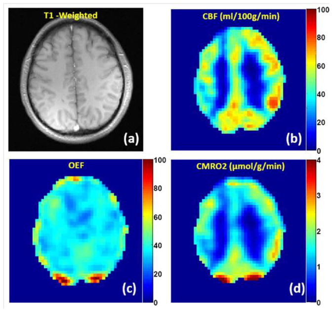
(adapted from (147)). Quantification of CMRO2 in healthy subject using ASL-qBOLD technique during the resting state. (a) T1-weighted anatomical image; (b) CBF map (in ml/100g/min) delineates the contrast between GM and WM; (c) OEF map is mostly uniform across the whole brain (two spots at the back of brain with extreme high OEF values correspond to large uncompensated B0 field inhomogeneities); (d) the map of CMRO2 (in μmol/g/min) demonstrates much higher value of CMRO2 in GM than in WM.
7. MR Susceptometry-based CMRO2 quantification
Simultaneous estimation of oxygen saturation and cerebral blood flow in the major vessels draining and feeding the brain can be used for rapid non-invasive quantification of whole-brain CMRO2. The vessel of interest often includes internal jugular vein and/or superior sagittal sinus (SSS). The principle of the MR susceptometry of the whole brain is based on the measurement of the susceptibility difference between blood in the draining vein (such as jugular vein or SSS), and its surrounding tissue by measuring the phase difference with a GRE sequence (field mapping) (91,115,151–153). The SSS is often preferred over the internal jugular vein where severe susceptibility artifacts, caused by the proximity of air spaces such as the oral cavity and trachea, may complicate measurements. An additional benefit of the SSS is the elimination of contamination by the blood from extra-cranial sources (144).
In (152), the draining vein was considered as a long cylinder with a fixed orientation relative to the static magnetic field B0. For such a model, the proton Larmor frequency is homogeneous within the cylinder (blood vessel), Eq. [23], and inhomogeneous outside the cylinder (surrounding tissue), Eq. [40]; however, the average frequency in the surrounding tissue is equal to 0 (due to the factor cos2φ in Eq. [40]). These frequencies are usually measured from a set of phase images acquired at different gradient echo times. A difference between gradient echo MR signal phase inside the vein and an average phase of MR signal in the tissue is equal to (see Eq. [23]):
| [73] |
where θ is the relative angle between blood vessel and the static magnetic field B0 and ΔTE is the interval between gradient echo times. The fraction of oxygenated hemoglobin Y can then be determined as (152):
| [74] |
This result corresponds to a simplified relationship between blood magnetic susceptibility and blood oxygenation level, Eq. [22]. Note that in (152), the SI units are used whereas in this paper we use Gaussian-CGS units. To reduce the phase artifacts from moving blood, a flow-compensated 2D GRE sequence is often adopted. Blood vessel curvature and tapering may produce potential deviations from the long cylinder model. To address this issue, the accuracy of the “long cylinder” approximation has been evaluated via numerical computation of the induced magnetic field from 3D segmented renditions of three veins of interest (superior sagittal sinus, femoral and jugular vein) (154). The authors concluded that at a typical venous oxygen saturation of 65%, the absolute error via a close-form cylinder approximation was only 2.6% when measured over three locations in three veins studied and did not exceed 5% for vessel tilt angles <300 at any location. The influence of vessel eccentricity was examined theoretically and experimentally in (155). The problem of macroscopic magnetic field inhomogeneities resulting in low spatial-frequency variations in the reference tissue was corrected in (156) by means of a polynomial approximation for a field map.
An example of this technique is illustrated in Figure 16 where GRE signal phase was quantified for a baseline state and during hypercapnia (91). Notice the expected decrease in phase contrast for the SSS, indicating increased blood oxygenation level during hypercapnia. To evaluate CMRO2, in addition to Eq.[74], the blood flow in the vein should also be quantified. In (152) CBF was quantified using a phase-contrast technique (63,157). With a separate CBF quantification by phase-contrast MRI, MR oximetry has been successfully applied to quantify global brain oxygen metabolism at baseline (152). The sensitivity of this technique has also been demonstrated during breath-holding and hypoventilation (115).
Figure 16.

(adapted from (91)). Images from which venous oxygen saturation during baseline, hypercapnia, and recovery were derived. (A) Sagittal localizer angiogram indicating the locations of SSS; (B) axial magnitude image; (C–E) GRE phase-difference images. Note the change in contrast in vessels during hypercapnia.
In pediatric traumatic brain injury (TBI) patients, depressed global brain OEF has also been observed, while global OEF measured within two weeks of injury was found to be predictive of patient outcome at 3 mo after injury (158). Susceptibility-based MR oximetry has also been adapted to quantify oxygen kinetics of skeletal muscle in peripheral arterial diseases (159,160). With the improvement of MR technique, the acquisition time has been reduced from 4 mins to ~30 seconds, making the technique suitable for studying the temporal variations in CMRO2 in response to physiological challenges (91). In a recent paper (153), the susceptibility-based blood oxygen saturation technique was extended to quantify oxygen levels in small vein segments within gray matter, thus opening an opportunity for measuring regional oxygen metabolism of brain tissue.
8. T2-based CMRO2 quantification
Another approach for quantifying biological tissue hemodynamic properties is based on measuring blood T2 relaxation that is related to blood oxygenation level (see Section 4.3 above). In (89), CPMG pulse sequence was used to measure the blood transverse relaxation rate constant, see Eq. [34]. The reduction in acquisition time when comparing a CPMG sequence with single SE sequences may provide advantages such as the reduction in the motion sensitivity of the T2 determination, and possible inter-scan differences in the physiological reactions to the stimulus (125).
One potential problem of the aforementioned approach is the possible signal contamination of intravascular blood from tissue and CSF/ISF signals due to partial volume effects (81), similarly as reported in (161). The isolation of pure venous blood signal is not a trivial task to carry out in vivo, even in large blood vessels such as the sagittal sinuses. The susceptibility to contamination by CSF/ISF space known as the arachnoid granulations often leads to non mono-exponential MR signal decay (162). In addition, the rapid movement of blood, especially in large vessels, presents a second technical challenge for studies seeking an accurate quantification of absolute blood oxygenation. To address these issues, Lu et al (162) proposed a spin-labeling technique, TRUST (T2-Relaxation-Under-Spin-Tagging), which can isolate pure venous blood signal (see also (163)). TRUST technique minimizes the partial volume effect and avoids the need for judicious selection of voxels containing blood. The T2 relaxation time of the TRUST signal can then be determined and converted to venous oxygenation Yv using a calibration plot (74,75,164). To minimize the outflow effect in blood T2 quantification, the T2-weighting of isolated blood signal in major blood vessels is often achieved by using a series of non-slice-selective T2-preparation pulses rather than the conventional spin-echo sequence. Figure 17 illustrated the TRUST sequence diagram (165). In (125) and (166), a non-selective saturation pulse was applied right after the signal acquisition to reset magnetization in the whole brain, thus improving the speed and reliability of TRUST MRI.
Figure 17.

(adapted from (162)) TRUST MRI technique Sequence diagram. (a) Pulse sequence diagram for TRUST MRI. The sequence consists of interleaved acquisitions of label and control scans, and each image type is acquired with four different effective TEs ranging from 0 to 160 ms. For each scan, the sequence starts with a presaturation RF pulse to suppress the static tissue signal, followed by a labeling (or control) RF pulse to magnetically label the incoming blood. A brief waiting period (1.2 seconds) is allowed for blood to flow into the imaging slice. Before data acquisition, a non-selective T2-preparation pulse train is applied to achieve the T2-weighting. The T2-preparation scheme, instead of conventional T2-weighted sequence, is used in order to minimize the blood outflow effect. (b) Positions of the imaging slice (yellow) and the labeling slab (green).
The theoretical framework of TRUST MRI is similar to that of ASL, but the scenario is simpler for TRUST MRI because the blood and static tissue compartments are strictly segregated (venous vessel walls are not permeable to water molecules) and there is no exchange effects during the inversion time. This technique has been validated in humans (164). It has shown promise for normalization of fMRI signals (162,167) and for studying cognitive aging (168) and multiple sclerosis (169). Methodological studies have also confirmed the sensitivity of this technique to physiologic procedures such as hypercapnia/hyperoxia (166) and caffeine uptake (162).
Spatial information is largely lost in TRUST or other T2-based approaches. Because of spatial resolution limitation, usable voxels are typically found only in large venous vessels. The QUIXOTIC (quantitative imaging of extraction of oxygen and tissue consumption) technique introduced by Bolar et al (170) separated the post-capillary venous blood signal from decelerating arterial blood and static tissue using velocity selective spin labeling (VSSL) technique. By measuring the T2 of this post-capillary blood, it is possible to generate the brain OEF thus CMRO2 maps, as shown in Figure 18 (170). Reliability of this approach was further improved in (171) by nulling the MR signal from inflow arterial blood and combining with phase sensitive signal detection. The improved method successfully detected the change of oxygenation during a hypoxia challenge.
Figure 18.

(adapted from (170)). An example of quantitative Yv (left), OEF (middle), and CMRO2 (right) maps obtained by QUIXOTIC technique.
9. Concluding Remarks
Studying brain hemodynamics and metabolism in health and disease attracts attention of scientists and clinicians, and numerous papers have been published on this subject. In this paper we review several BOLD-based experimental MR methods for studying brain function and discuss in detail theoretical background behind these techniques. These techniques allow evaluation of OEF through measuring blood oxygenation levels and (in combination with measuring CBF) estimation of CMRO2. Of course, in a single review it is impossible to even mention all publications on this issue and our list of references is far from being exhaustive. A direct measurement of CMRO2 is also possible by using tracers such as 17O2. This novel technique was described in detail in a recent review (172) and therefore is not discussed in our paper. We also have not included numerous publications aimed at measuring changes in brain hemodynamics and metabolism during functional activation as they are discussed in other articles of this special issue of NMR in Biomedicine. The present paper gives an updated picture of recently developed MR-based approaches for quantifying brain OEF, dCBV and CMRO2 properties1.
Figure 12.

(adapted from (86)). Histograms of the estimated brain parameters for the study shown in Fig. 11. The histograms represent dCBV (%), OEF (%), CSF/ISF volume fraction, CSF/ISF frequency shift (Hz); R2 of the brain tissue (s−1), and the concentration of deoxyhemoglobin (μM).
Acknowledgments
The authors are grateful to Professors Marcus Raichle, Felix Wehrli, Hanzhang Lu, Mark Conradi and Joseph Ackerman for helpful discussions. This work was supported by NIH grant R01 NS 055963.
Footnotes
When this paper was in revision, two publications devoted to development of yet another method for quantification of brain metabolism appeared in press (173, 174). They are based on an extension of the so-called calibrated fMRI approach (175, 176). A detail discussion of this method can be found in (177), see also related publications (148, 178–180).
References
- 1.Raichle ME, Mintun MA. Brain work and brain imaging. Annu Rev Neurosci. 2006;29:449–476. doi: 10.1146/annurev.neuro.29.051605.112819. [DOI] [PubMed] [Google Scholar]
- 2.Derdeyn CP, Videen TO, Yundt KD, Fritsch SM, Carpenter DA, Grubb RL, Powers WJ. Variability of cerebral blood volume and oxygen extraction: stages of cerebral haemodynamic impairment revisited. Brain. 2002;125(Pt 3):595–607. doi: 10.1093/brain/awf047. [DOI] [PubMed] [Google Scholar]
- 3.Iadecola C. Neurovascular regulation in the normal brain and in Alzheimer’s disease. Nat Rev Neurosci. 2004;5(5):347–360. doi: 10.1038/nrn1387. [DOI] [PubMed] [Google Scholar]
- 4.Iadecola C. Rescuing troubled vessels in Alzheimer disease. Nat Med. 2005;11(9):923–924. doi: 10.1038/nm0905-923. [DOI] [PubMed] [Google Scholar]
- 5.Vlassenko AG, Vaishnavi SN, Couture L, Sacco D, Shannon BJ, Mach RH, Morris JC, Raichle ME, Mintun MA. Spatial correlation between brain aerobic glycolysis and amyloid-beta (Abeta) deposition. Proc Natl Acad Sci U S A. 2010;107(41):17763–17767. doi: 10.1073/pnas.1010461107. [DOI] [PMC free article] [PubMed] [Google Scholar]
- 6.Powers WJ, Videen TO, Markham J, McGee-Minnich L, Antenor-Dorsey JV, Hershey T, Perlmutter JS. Selective defect of in vivo glycolysis in early Huntington’s disease striatum. Proc Natl Acad Sci U S A. 2007;104(8):2945–2949. doi: 10.1073/pnas.0609833104. [DOI] [PMC free article] [PubMed] [Google Scholar]
- 7.Beal MF. Mitochondrial dysfunction in neurodegenerative diseases. Biochim Biophys Acta. 1998;1366(1–2):211–223. doi: 10.1016/s0005-2728(98)00114-5. [DOI] [PubMed] [Google Scholar]
- 8.Schapira AH. Mitochondrial dysfunction in neurodegenerative disorders. Biochim Biophys Acta. 1998;1366(1–2):225–233. doi: 10.1016/s0005-2728(98)00115-7. [DOI] [PubMed] [Google Scholar]
- 9.Leenders KL, Frackowiak RS, Quinn N, Marsden CD. Brain energy metabolism and dopaminergic function in Huntington’s disease measured in vivo using positron emission tomography. Mov Disord. 1986;1(1):69–77. doi: 10.1002/mds.870010110. [DOI] [PubMed] [Google Scholar]
- 10.Santens P, De Reuck J, Crevits L, Decoo D, Lemahieu I, Strijckmans K, Goethals P. Cerebral oxygen metabolism in patients with progressive supranuclear palsy: a positron emission tomography study. Eur Neurol. 1997;37(1):18–22. doi: 10.1159/000117398. [DOI] [PubMed] [Google Scholar]
- 11.Shishido F, Uemura K, Inugami A, Tomura N, Higano S, Fujita H, Sasaki H, Kanno I, Murakami M, Watahiki Y, Nagata K. Cerebral oxygen and glucose metabolism and blood flow in mitochondrial encephalomyopathy: a PET study. Neuroradiology. 1996;38(2):102–107. doi: 10.1007/BF00604789. [DOI] [PubMed] [Google Scholar]
- 12.Tanaka M, Kondo S, Okamoto K, Hirai S. [Cerebral perfusion and oxygen metabolism in Parkinson’s disease: positron emission tomographic study using oxygen-15-labeled CO2 and O2] Nihon Rinsho. 1997;55(1):218–221. [PubMed] [Google Scholar]
- 13.Tatum JL, Kelloff GJ, Gillies RJ, Arbeit JM, Brown JM, Chao KS, Chapman JD, Eckelman WC, Fyles AW, Giaccia AJ, Hill RP, Koch CJ, Krishna MC, Krohn KA, Lewis JS, Mason RP, Melillo G, Padhani AR, Powis G, Rajendran JG, Reba R, Robinson SP, Semenza GL, Swartz HM, Vaupel P, Yang D, Croft B, Hoffman J, Liu G, Stone H, Sullivan D. Hypoxia: importance in tumor biology, noninvasive measurement by imaging, and value of its measurement in the management of cancer therapy. Int J Radiat Biol. 2006;82(10):699–757. doi: 10.1080/09553000601002324. [DOI] [PubMed] [Google Scholar]
- 14.Davda S, Bezabeh T. Advances in methods for assessing tumor hypoxia in vivo: implications for treatment planning. Cancer Metastasis Rev. 2006;25(3):469–480. doi: 10.1007/s10555-006-9009-z. [DOI] [PubMed] [Google Scholar]
- 15.Ogawa S, Lee T, Kay A, Tank D. Brain magnetic resonance imaging with contrast dependent on blood oxygenation. Proc Natl Acad Sci (USA) 1990;87:868–9872. doi: 10.1073/pnas.87.24.9868. [DOI] [PMC free article] [PubMed] [Google Scholar]
- 16.Ogawa S, Tank D, Menon R, Ellermann J, Kim S-G, Merkle H, Ugurbil K. Intrinsic signal changes accompanying sensory stimulation: functional brain mapping with magnetic resonance imaging. Proc Natl Acad Sci (USA) 1992;89:5951–5955. doi: 10.1073/pnas.89.13.5951. [DOI] [PMC free article] [PubMed] [Google Scholar]
- 17.Bandettini P, Wong E, Hinks R, Tikofsky R, Hyde J. Time course EPI of human brain function during task activation. Mag Res Med. 1992;25:390–397. doi: 10.1002/mrm.1910250220. [DOI] [PubMed] [Google Scholar]
- 18.Kwong K, Belliveau J, Chesler D, Goldberg I, Weiskoff R, Poncelet B, Kennedy D, Hoppel B, Cohen M, Turner R, Cheng H-M, Brady T, Rosen B. Dynamic magnetic resonance imaging of human brain activity during primary sensory stimulation. Proc Natl Acad Sci (USA) 1992;89:5675–5679. doi: 10.1073/pnas.89.12.5675. [DOI] [PMC free article] [PubMed] [Google Scholar]
- 19.Frahm J, Merboldt KD, Hanicke W. Functional MRI of human brain activation at high spatial resolution. Magn Reson Med. 1993;29(1):139–144. doi: 10.1002/mrm.1910290126. [DOI] [PubMed] [Google Scholar]
- 20.Raichle ME, MacLeod AM, Snyder AZ, Powers WJ, Gusnard DA. A default mode of brain function. Proc Natl Acad Sci U S A. 2001;98(2):676–682. doi: 10.1073/pnas.98.2.676. [DOI] [PMC free article] [PubMed] [Google Scholar]
- 21.Gusnard DA, Raichle ME. Searching for a baseline: functional imaging and the resting human brain. Nat Rev Neurosci. 2001;2(10):685–694. doi: 10.1038/35094500. [DOI] [PubMed] [Google Scholar]
- 22.Powers WJ, Grubb RL, Jr, Darriet D, Raichle ME. Cerebral blood flow and cerebral metabolic rate of oxygen requirements for cerebral function and viability in humans. J Cereb Blood Flow Metab. 1985;5(4):600–608. doi: 10.1038/jcbfm.1985.89. [DOI] [PubMed] [Google Scholar]
- 23.Derdeyn CP, Grubb RL, Jr, Powers WJ. Cerebral hemodynamic impairment: methods of measurement and association with stroke risk. Neurology. 1999;53(2):251–259. doi: 10.1212/wnl.53.2.251. [DOI] [PubMed] [Google Scholar]
- 24.Powers WJ. Cerebral hemodynamics in ischemic cerebrovascular disease. Ann Neurol. 1991;29(3):231–240. doi: 10.1002/ana.410290302. [DOI] [PubMed] [Google Scholar]
- 25.Yamauchi H, Fukuyama H, Nagahama Y, Nabatame H, Nakamura K, Yamamoto Y, Yonekura Y, Konishi J, Kimura J. Evidence of misery perfusion and risk for recurrent stroke in major cerebral arterial occlusive diseases from PET. J Neurol Neurosurg Psychiatry. 1996;61(1):18–25. doi: 10.1136/jnnp.61.1.18. [DOI] [PMC free article] [PubMed] [Google Scholar]
- 26.Grubb RL, Jr, Derdeyn CP, Fritsch SM, Carpenter DA, Yundt KD, Videen TO, Spitznagel EL, Powers WJ. Importance of hemodynamic factors in the prognosis of symptomatic carotid occlusion. Jama. 1998;280(12):1055–1060. doi: 10.1001/jama.280.12.1055. [DOI] [PubMed] [Google Scholar]
- 27.Kety SS, Schmidt CF. The effects of altered arterial tensions of carbon dioxide and oxygen on cerebral blood flow and cerebral oxygen consumption of normal young men. J Clin Invest. 1948;27:484–491. doi: 10.1172/JCI101995. [DOI] [PMC free article] [PubMed] [Google Scholar]
- 28.West JB. Respiratory Physiology. The essentials. Philadelphia, PA: Lippincott Williams & Wilkins; 1999. [Google Scholar]
- 29.Schwarzbauer C, Deichmann R. Vascular component analysis of hyperoxic and hypercapnic BOLD contrast. Neuroimage. 2012;59(3):2401–2412. doi: 10.1016/j.neuroimage.2011.08.110. [DOI] [PubMed] [Google Scholar]
- 30.Hillman R, Finch C. The red cell manual. Philadelphia: F.A. Davis, Co; 1996. [Google Scholar]
- 31.Dickerson R, Gies I. Hemoglobin: structure, function, evolution and pathology. Menlo Park, CA: Benjamin-Cummings Publishing; 1994. [Google Scholar]
- 32.Schenck JF. Magnetic resonance imaging of brain iron. J Neurol Sci. 2003;207(1–2):99–102. doi: 10.1016/s0022-510x(02)00431-8. [DOI] [PubMed] [Google Scholar]
- 33.Schenck JF, Zimmerman EA. High-field magnetic resonance imaging of brain iron: birth of a biomarker? NMR Biomed. 2004;17(7):433–445. doi: 10.1002/nbm.922. [DOI] [PubMed] [Google Scholar]
- 34.Haacke EM, Cheng NY, House MJ, Liu Q, Neelavalli J, Ogg RJ, Khan A, Ayaz M, Kirsch W, Obenaus A. Imaging iron stores in the brain using magnetic resonance imaging. Magn Reson Imaging. 2005;23(1):1–25. doi: 10.1016/j.mri.2004.10.001. [DOI] [PubMed] [Google Scholar]
- 35.Pauling L, Coryell C. The magnetic properties and structure of the hemochromogens and related substances. Proc Natl Acad Sci USA. 1936;22:159–163. doi: 10.1073/pnas.22.3.159. [DOI] [PMC free article] [PubMed] [Google Scholar]
- 36.Pauling L, Coryell CD. The magnetic properties and structure of hemoglobin, oxyhemoglobin and carbonmonoxyhemoglobin. Proc Natl Acad Sci USA. 1936;22:210–216. doi: 10.1073/pnas.22.4.210. [DOI] [PMC free article] [PubMed] [Google Scholar]
- 37.Thulborn KR, Waterton JC, Matthews PM, Radda GK. Oxygenation dependence of the transverse relaxation time of waterprotons in whole blood at high field. Biochim et Biophys Acta. 1982;714:265–270. doi: 10.1016/0304-4165(82)90333-6. [DOI] [PubMed] [Google Scholar]
- 38.Ogawa S, Lee T, Nayak AS, Glynn P. Oxygenation-sensitive contrast in magnetic resonance image of rodent brain at high fields. Magn Reson Med. 1990;14:68–78. doi: 10.1002/mrm.1910140108. [DOI] [PubMed] [Google Scholar]
- 39.Poon CS, Henkelman RM. Practical T2 quantitation for clinical applications. J Magn Reson Imaging. 1992;2(5):541–553. doi: 10.1002/jmri.1880020512. [DOI] [PubMed] [Google Scholar]
- 40.Carr HY, Purcell EM. Effects of Diffusion on Free Precession in Nuclear Magnetic Resonance Experiments. Phys Rev. 1954;94(3):630–638. [Google Scholar]
- 41.Luz Z, Meiboom S. Nuclear magnetic resonance study of protolysis of trimethylammonium ion in aqueous solution - order of reaction with respect to solvent. J Chem Phys. 1963;39:366–370. [Google Scholar]
- 42.Yablonskiy DA, Haacke EM. Theory of NMR signal behavior in magnetically inhomogeneous tissues: the static dephasing regime. Magn Reson Med. 1994;32:749–763. doi: 10.1002/mrm.1910320610. [DOI] [PubMed] [Google Scholar]
- 43.Yablonskiy DA. Quantitation of Intrinsic Magnetic Susceptibility-Related Effects in a Tissue Matrix. Phantom Study. Magn Reson Med. 1998;39:417–428. doi: 10.1002/mrm.1910390312. [DOI] [PubMed] [Google Scholar]
- 44.Stables LA, Kennan RP, Gore JC. Asymmetric spin-echo imaging of magnetically inhomogeneous systems: theory, experiment, and numerical studies. Magn Reson Med. 1998;40(3):432–442. doi: 10.1002/mrm.1910400314. [DOI] [PubMed] [Google Scholar]
- 45.Kiselev VG, Posse S. Analytical Theory of Susceptibility Induced NMR Signal Dephasing in a Celebrovascular Network. Phys Rev Lett. 1998;81(25):5696–5699. [Google Scholar]
- 46.Kiselev VG, Posse S. Analytical model of susceptibility-induced MR signal dephasing: effect of diffusion in a microvascular network. Magn Reson Med. 1999;41(3):499–509. doi: 10.1002/(sici)1522-2594(199903)41:3<499::aid-mrm12>3.0.co;2-o. [DOI] [PubMed] [Google Scholar]
- 47.Bauer WR, Nadler W, Bock M, Schad LR, Wacker C, Hartlep A, Ertl G. Theory of the BOLD effect in the capillary region: an analytical approach for the determination of T2 in the capillary network of myocardium. Magn Reson Med. 1999;41(1):51–62. doi: 10.1002/(sici)1522-2594(199901)41:1<51::aid-mrm9>3.0.co;2-g. [DOI] [PubMed] [Google Scholar]
- 48.Bauer WR, Nadler W. Spin dephasing in the extended strong collision approximation. Phys Rev E. 2002;65:066123. doi: 10.1103/PhysRevE.65.066123. [DOI] [PubMed] [Google Scholar]
- 49.Jensen JH, Chandra R. Strong Field Behaviour of the NMR Signal from Magnetically Heterogeneous Tissues. Magn Reson Med. 2000;43:226–236. doi: 10.1002/(sici)1522-2594(200002)43:2<226::aid-mrm9>3.0.co;2-p. [DOI] [PubMed] [Google Scholar]
- 50.Jensen JH, Chandra R. NMR Relaxation in Tissues with Weak Magnetic Inhomogeneities. Magn Reson Med. 2000;44:144–156. [PubMed] [Google Scholar]
- 51.Kiselev VG, Novikov DS. Theory of MR Relaxation Caused by Mesoscopic Impuritues: a Possibility to Monitor the Red Blood Cell Shape. Glasgow, Scottland: 2001. [Google Scholar]
- 52.Sukstanskii AL, Yablonskiy DA. Theory of FID NMR signal dephasing induced by mesoscopic magnetic field inhomogeneities in biological systems. J Magn Reson. 2001;151(1):107–117. doi: 10.1006/jmre.2001.2363. [DOI] [PubMed] [Google Scholar]
- 53.Sukstanskii AL, Yablonskiy DA. Gaussian approximation in the theory of MR signal formation in the presence of structure-specific magnetic field inhomogeneities. J Magn Reson. 2003;163(2):236–247. doi: 10.1016/s1090-7807(03)00131-9. [DOI] [PubMed] [Google Scholar]
- 54.Sukstanskii AL, Yablonskiy DA. Gaussian approximation in the theory of MR signal formation in the presence of structure-specific magnetic field inhomogeneities. Effects of impermeable susceptibility inclusions. J Magn Reson. 2004;167(1):56–67. doi: 10.1016/j.jmr.2003.11.006. [DOI] [PubMed] [Google Scholar]
- 55.Fujita N, Shinohara M, Tanaka H, Yutani K, Nakamura H, Murase K. Quantitative mapping of cerebral deoxyhemoglobin content using MR imaging. Neuroimage. 2003;20(4):2071–2083. doi: 10.1016/j.neuroimage.2003.06.002. [DOI] [PubMed] [Google Scholar]
- 56.Frohlich AF, Ostergaard L, Kiselev VG. Theory of susceptibility-induced transverse relaxation in the capillary network in the diffusion narrowing regime. Magn Reson Med. 2005;53(3):564–573. doi: 10.1002/mrm.20394. [DOI] [PubMed] [Google Scholar]
- 57.Novikov DS, Kiselev VG. Transverse NMR relaxation in magnetically heterogeneous media. J Magn Reson. 2008;195(1):33–39. doi: 10.1016/j.jmr.2008.08.005. [DOI] [PubMed] [Google Scholar]
- 58.Novikov DS, Kiselev VG. Effective medium theory of a diffusion-weighted signal. NMR in Biomedicine. 2010;23(7):682–697. doi: 10.1002/nbm.1584. [DOI] [PubMed] [Google Scholar]
- 59.Cerdonio M, Congiu-Castellano A, Calabrese L, Morante S, Pispisa B, Vitale S. Room-temperature magnetic properties of oxy- and carbonmonoxyhemoglobin. Proc Natl Acad Sci U S A. 1978;75(10):4916–4919. doi: 10.1073/pnas.75.10.4916. [DOI] [PMC free article] [PubMed] [Google Scholar]
- 60.Plyavin YA, Blum EY. Magnetic parameters of blood cells and high-gradient paramagnetic and diamagnetic phoresis. Magnetohydrodynamics. 1983;19:349–359. [Google Scholar]
- 61.Brooks RA, Di Chiro G. Magnetic resonance imaging of stationary blood: a review. Med Phys. 1987;14(6):903–913. doi: 10.1118/1.595994. [DOI] [PubMed] [Google Scholar]
- 62.Gomori JM, Grossman RI, Yu-Ip C, Asakura T. NMR relaxation times of blood: dependence on field strength, oxidation state, and cell integrity. J Comput Assist Tomogr. 1987;11(4):684–690. [PubMed] [Google Scholar]
- 63.Bryant RG, Marill K, Blackmore C, Francis C. Magnetic relaxation in blood and blood clots. Magn Reson Med. 1990;13(1):133–144. doi: 10.1002/mrm.1910130112. [DOI] [PubMed] [Google Scholar]
- 64.Gasparovic C, Matwiyoff NA. The magnetic properties and water dynamics of the red blood cell: a study by proton-NMR lineshape analysis. Magn Reson Med. 1992;26(2):274–299. doi: 10.1002/mrm.1910260208. [DOI] [PubMed] [Google Scholar]
- 65.Matwiyoff NA, Gasparovic C, Mazurchuk R, Matwiyoff G. The line shapes of the water proton resonances of red blood cells containing carbonyl hemoglobin, deoxyhemoglobin, and methemoglobin: implications for the interpretation of proton MRI at fields of 1. 5 T and below. Magn Reson Imaging. 1990;8(3):295–301. doi: 10.1016/0730-725x(90)90102-8. [DOI] [PubMed] [Google Scholar]
- 66.Wright GA, Hu BS, Macovski A. Estimating oxygen saturation of blood in vivo with MR imaging at 1. 5 T. J Magn Reson Imaging. 1991;1(3):275–283. doi: 10.1002/jmri.1880010303. [DOI] [PubMed] [Google Scholar]
- 67.Weisskoff RM, Kiihne S. MRI susceptometry: Image-based measurement of absolute susceptibility of MR contrast agents and human blood. Magn Reson Med. 1992;24:375–383. doi: 10.1002/mrm.1910240219. [DOI] [PubMed] [Google Scholar]
- 68.Meyer ME, Yu O, Eclancher B, Grucker D, Chambron J. NMR relaxation rates and blood oxygenation level. Magn Reson Med. 1995;34(2):234–241. doi: 10.1002/mrm.1910340215. [DOI] [PubMed] [Google Scholar]
- 69.Chien D, Levin DL, Anderson CM. MR gradient echo imaging of intravascular blood oxygenation: T2* determination in the presence of flow. Magn Reson Med. 1994;32(4):540–545. doi: 10.1002/mrm.1910320419. [DOI] [PubMed] [Google Scholar]
- 70.Kuchel PW, Fackerell ED. Parametric-equation representation of biconcave erythrocytes. Bull Math Biol. 1999;61(2):209–220. doi: 10.1006/bulm.1998.0064. [DOI] [PubMed] [Google Scholar]
- 71.Spees WM, Yablonskiy DA, Oswood MC, Ackerman JJH. MR Properties of Human Blood at 1.5 Tesla, T1, T2, T2* and Gaussian Relaxation Behavior. Magn Reson Med. 2001;45:533–542. doi: 10.1002/mrm.1072. [DOI] [PubMed] [Google Scholar]
- 72.Yablonskiy DA, Sukstanskii AL, Springer CS, Ackerman JJH. Theory of 1H20 T2 Relaxation in Blood. Proceedings of the 11th ISMRM Conference; 2003; Toronto, Canada. [Google Scholar]
- 73.Kjolby BF, Ostergaard L, Kiselev VG. Theoretical model of intravascular paramagnetic tracers effect on tissue relaxation. Magn Reson Med. 2006;56(1):187–197. doi: 10.1002/mrm.20920. [DOI] [PubMed] [Google Scholar]
- 74.Silvennoinen MJ, Clingman CS, Golay X, Kauppinen RA, van Zijl PC. Comparison of the dependence of blood R2 and R2* on oxygen saturation at 1.5 and 4. 7 Tesla. Magn Reson Med. 2003;49(1):47–60. doi: 10.1002/mrm.10355. [DOI] [PubMed] [Google Scholar]
- 75.Zhao JM, Clingman CS, Narvainen MJ, Kauppinen RA, van Zijl PC. Oxygenation and hematocrit dependence of transverse relaxation rates of blood at 3T. Magn Reson Med. 2007;58(3):592–597. doi: 10.1002/mrm.21342. [DOI] [PubMed] [Google Scholar]
- 76.Qin Q, Grgac K, van Zijl PC. Determination of whole-brain oxygen extraction fractions by fast measurement of blood T(2) in the jugular vein. Magn Reson Med. 2011;65(2):471–479. doi: 10.1002/mrm.22556. [DOI] [PMC free article] [PubMed] [Google Scholar]
- 77.Jain V, Abdulmalik O, Propert KJ, Wehrli FW. Investigating the magnetic susceptibility properties of fresh human blood for noninvasive oxygen saturation quantification. Magn Reson Med. 2012 doi: 10.1002/mrm.23282. [DOI] [PMC free article] [PubMed] [Google Scholar]
- 78.Hoppel BE, Weisskoff RM, Thulborn KR, Moore JB, Kwong KK, Rosen BR. Measurement of regional blood oxygenation and cerebral hemodynamics. Magn Reson Med. 1993;30(6):715–723. doi: 10.1002/mrm.1910300609. [DOI] [PubMed] [Google Scholar]
- 79.Cerdonio M, Morante S, Vitale S. Magnetic susceptibility of hemoglobins. Methods Enzymol. 1981;76:354–371. doi: 10.1016/0076-6879(81)76131-7. [DOI] [PubMed] [Google Scholar]
- 80.Vander A, Sherman J, Luciano D. Human physiology. New York: McGraw-Hill; 1994. [Google Scholar]
- 81.Golay X, Silvennoinen MJ, Zhou J, Clingman CS, Kauppinen RA, Pekar JJ, van Zij PC. Measurement of tissue oxygen extraction ratios from venous blood T(2): increased precision and validation of principle. Magn Reson Med. 2001;46(2):282–291. doi: 10.1002/mrm.1189. [DOI] [PubMed] [Google Scholar]
- 82.He X, Yablonskiy DA. Biophysical mechanisms of phase contrast in gradient echo MRI. Proc Natl Acad Sci U S A. 2009;106(32):13558–13563. doi: 10.1073/pnas.0904899106. [DOI] [PMC free article] [PubMed] [Google Scholar]
- 83.Ogawa S, Lee TM, Barrere B. The sensitivity of magnetic resonance image signals of a rat brain to changes in the cerebral venous blood oxygenation. Magn Reson Med. 1993;29(2):205–210. doi: 10.1002/mrm.1910290208. [DOI] [PubMed] [Google Scholar]
- 84.Chu SC-K, Xu Y, Balschi JA, Springer CS. Bulk magnetic susceptibility shift in NMR studies of compartmentalized samples: use of paramagnetic reagents. Magn Reson Med. 1990;13:239–262. doi: 10.1002/mrm.1910130207. [DOI] [PubMed] [Google Scholar]
- 85.Lauwers F, Cassot F, Lauwers-Cances V, Puwanarajah P, Duvernoy H. Morphometry of the human cerebral cortex microcirculation: general characteristics and space-related profiles. Neuroimage. 2008;39(3):936–948. doi: 10.1016/j.neuroimage.2007.09.024. [DOI] [PubMed] [Google Scholar]
- 86.He X, Yablonskiy DA. Quantitative BOLD: mapping of human cerebral deoxygenated blood volume and oxygen extraction fraction: default state. Magn Reson Med. 2007;57(1):115–126. doi: 10.1002/mrm.21108. [DOI] [PMC free article] [PubMed] [Google Scholar]
- 87.Abramowitz M, Stegun IA. Handbook of Mathematical Functions. New York: Dover Publications, Inc; 1972. [Google Scholar]
- 88.Gradstein IS, Ryzhik IM. Russian by Scripta Technica I. In: Table of Integrals, Series, and Products. Jeffrey A, editor. NY: Academic Press; 1999. [Google Scholar]
- 89.Oja JM, Gillen JS, Kauppinen RA, Kraut M, van Zijl PC. Determination of oxygen extraction ratios by magnetic resonance imaging. J Cereb Blood Flow Metab. 1999;19(12):1289–1295. doi: 10.1097/00004647-199912000-00001. [DOI] [PubMed] [Google Scholar]
- 90.Fung YC, Tsang WCO, Patitucci P. High-Resolution Data on the Geometry of Red Blood Cells. Biorheology. 1981;18:369–385. doi: 10.3233/bir-1981-183-606. [DOI] [PubMed] [Google Scholar]
- 91.Jain V, Langham MC, Floyd TF, Jain G, Magland JF, Wehrli FW. Rapid magnetic resonance measurement of global cerebral metabolic rate of oxygen consumption in humans during rest and hypercapnia. J Cereb Blood Flow Metab. 2011;31(7):1504–1512. doi: 10.1038/jcbfm.2011.34. [DOI] [PMC free article] [PubMed] [Google Scholar]
- 92.van Zijl PC, Eleff SM, Ulatowski JA, Oja JM, Ulug AM, Traystman RJ, Kauppinen RA. Quantitative assessment of blood flow, blood volume and blood oxygenation effects in functional magnetic resonance imaging. Nat Med. 1998;4(2):159–167. doi: 10.1038/nm0298-159. [DOI] [PubMed] [Google Scholar]
- 93.Gardener AG, Francis ST, Prior M, Peters A, Gowland PA. Dependence of blood R2 relaxivity on CPMG echo-spacing at 2. 35 and 7 T. Magn Reson Med. 2010;64(4):967–974. doi: 10.1002/mrm.22575. [DOI] [PubMed] [Google Scholar]
- 94.Allerhand A, Gutowsky HS. Spin-echo NMR studies of chemical exchange. 1. Some general aspects. J Chem Phys. 1964;41:2115–2126. doi: 10.1063/1.1696165. [DOI] [PubMed] [Google Scholar]
- 95.Allerhand A, Gutowsky HS. Spin-Echo Studies of Chemical Exchange. 2. Closed Formulas for Two Sites. J Chem Phys. 1965;42:1587–1599. doi: 10.1063/1.1696165. [DOI] [PubMed] [Google Scholar]
- 96.Slichter CP. Principles of Magnetic Resonance. Berlin: Springer_Verlag; 1990. p. 655. [Google Scholar]
- 97.Kiselev VG. Transverse relaxation effect of MRI contrast agents: a crucial issue for quantitative measurements of cerebral perfusion. J Magn Reson Imaging. 2005;22(6):693–696. doi: 10.1002/jmri.20452. [DOI] [PubMed] [Google Scholar]
- 98.Boxerman JL, Hamberg LM, Rosen BR, Weisskoff RM. MR Contrast due to Intravascular Magnetic Susceptibility Perturbations. Magn Reson Med. 1995;34:555–566. doi: 10.1002/mrm.1910340412. [DOI] [PubMed] [Google Scholar]
- 99.Uludag K, Muller-Bierl B, Ugurbil K. An integrative model for neuronal activity-induced signal changes for gradient and spin echo functional imaging. Neuroimage. 2009;48(1):150–165. doi: 10.1016/j.neuroimage.2009.05.051. [DOI] [PubMed] [Google Scholar]
- 100.Dickson JD, Ash TW, Williams GB, Sukstanskii AL, Ansorge RE, Yablonskiy DA. Quantitative phenomenological model of the BOLD contrast mechanism. J Magn Reson. 2011;212(1):17–25. doi: 10.1016/j.jmr.2011.06.003. [DOI] [PMC free article] [PubMed] [Google Scholar]
- 101.Jensen JH, Chandra R. MR imaging of microvasculature. Magn Reson Med. 2000;44(2):224–230. doi: 10.1002/1522-2594(200008)44:2<224::aid-mrm9>3.0.co;2-m. [DOI] [PubMed] [Google Scholar]
- 102.Christen T, Zaharchuk G, Pannetier N, Serduc R, Joudiou N, Vial JC, Remy C, Barbier EL. Quantitative MR estimates of blood oxygenation based on T(2) *: A numerical study of the impact of model assumptions. Magn Reson Med. 2012;67(5):1458–1468. doi: 10.1002/mrm.23094. [DOI] [PubMed] [Google Scholar]
- 103.Douglass DC, McCall DW. Diffusion in paraffin hydrocarbons. J Phys Chem. 1958;62:1102–1107. [Google Scholar]
- 104.Neuman CH. Spin echo of spin diffusion in a bounded medium. J Chem Phys. 1973;60(11):4508–4511. [Google Scholar]
- 105.Callaghan PT. Principles of Nuclear Magnetic Resonance Microscopy. NY: Claredon Press, Oxford; 1991. [Google Scholar]
- 106.Stepisnik J. Validity limits of Gaussian approximation in cumulant expansion for diffusion attenuation of spin echo. Physica B. 1999;270:110–117. [Google Scholar]
- 107.Sukstanskii AL, Yablonskiy DA. Effects of restricted diffusion on MR signal formation. J Magn Reson. 2002;157(1):92–105. doi: 10.1006/jmre.2002.2582. [DOI] [PubMed] [Google Scholar]
- 108.Yablonskiy DA, Sukstanskii AL. Theoretical models of the diffusion weighted MR signal. NMR Biomed. 2010;23(7):661–681. doi: 10.1002/nbm.1520. [DOI] [PMC free article] [PubMed] [Google Scholar]
- 109.Kiselev VG, Novikov DS. Transverse NMR relaxation as a probe of mesoscopic structure. Phys Rev Lett. 2002;89(27):278101. doi: 10.1103/PhysRevLett.89.278101. [DOI] [PubMed] [Google Scholar]
- 110.Martindale J, Kennerley AJ, Johnston D, Zheng Y, Mayhew JE. Theory and generalization of Monte Carlo models of the BOLD signal source. Magn Reson Med. 2008;59(3):607–618. doi: 10.1002/mrm.21512. [DOI] [PubMed] [Google Scholar]
- 111.Dickson JD, Ash TWJ, Williams GB, Harding SG, Carpenter TA, Menon DK, Ansorge RE. Quantitative BOLD: The Effect of Diffusion. J Magn Reson Imaging. 2010;32(4):953–961. doi: 10.1002/jmri.22151. [DOI] [PubMed] [Google Scholar]
- 112.He X, Zhu M, Yablonskiy DA. Validation of oxygen extraction fraction measurement by qBOLD technique. Magn Reson Med. 2008;60(4):882–888. doi: 10.1002/mrm.21719. [DOI] [PMC free article] [PubMed] [Google Scholar]
- 113.Yablonskiy DA. Quantitation of the Structure of Tissue Matrix from Intrinsic Magnetic Susceptibility Effects. Vancouver; Canada: 1997. p. 1559. [Google Scholar]
- 114.Ma J, Wehrli FW. Method for image-based measurement of the reversible and irreversible contribution to the transverse-relaxation rate. J Magn Reson B. 1996;111(1):61–69. doi: 10.1006/jmrb.1996.0060. [DOI] [PubMed] [Google Scholar]
- 115.Fernandez-Seara MA, Techawiboonwong A, Detre JA, Wehrli FW. MR susceptometry for measuring global brain oxygen extraction. Magn Reson Med. 2006;55(5):967–973. doi: 10.1002/mrm.20892. [DOI] [PubMed] [Google Scholar]
- 116.An H, Lin W. Quantitative measurements of cerebral blood oxygen saturation using magnetic resonance imaging. J Cereb Blood Flow Metab. 2000;20(8):1225–1236. doi: 10.1097/00004647-200008000-00008. [DOI] [PMC free article] [PubMed] [Google Scholar]
- 117.An H, Lin W. Cerebral oxygen extraction fraction and cerebral venous blood volume measurements using MRI: effects of magnetic field variation. Magn Reson Med. 2002;47(5):958–966. doi: 10.1002/mrm.10148. [DOI] [PubMed] [Google Scholar]
- 118.An H, Lin W. Impact of intravascular signal on quantitative measures of cerebral oxygen extraction and blood volume under normo- and hypercapnic conditions using an asymmetric spin echo approach. Magn Reson Med. 2003;50(4):708–716. doi: 10.1002/mrm.10576. [DOI] [PubMed] [Google Scholar]
- 119.Ansorge RE, Carpenter DA, Harding SG, Satangput P. Quantitative measurements of oxygen extraction fraction at 3T. Toronto, Canada: 2003. [Google Scholar]
- 120.Lu H, Golay X, van Zijl PC. Intervoxel heterogeneity of event-related functional magnetic resonance imaging responses as a function of T(1) weighting. Neuroimage. 2002;17(2):943–955. [PubMed] [Google Scholar]
- 121.Lu H, Golay X, Pekar JJ, Van Zijl PC. Sustained poststimulus elevation in cerebral oxygen utilization after vascular recovery. J Cereb Blood Flow Metab. 2004;24(7):764–770. doi: 10.1097/01.WCB.0000124322.60992.5C. [DOI] [PubMed] [Google Scholar]
- 122.Lu H, van Zijl PC. Experimental measurement of extravascular parenchymal BOLD effects and tissue oxygen extraction fractions using multi-echo VASO fMRI at 1.5 and 3. 0 T. Magn Reson Med. 2005;53(4):808–816. doi: 10.1002/mrm.20379. [DOI] [PubMed] [Google Scholar]
- 123.Whittall KP, MacKay AL, Graeb DA, Nugent RA, Li DK, Paty DW. In vivo measurement of T2 distributions and water contents in normal human brain. Magn Reson Med. 1997;37(1):34–43. doi: 10.1002/mrm.1910370107. [DOI] [PubMed] [Google Scholar]
- 124.Bender B, Klose U. Cerebrospinal fluid and interstitial fluid volume measurements in the human brain at 3T with EPI. Magn Reson Med. 2009;61(4):834–841. doi: 10.1002/mrm.21915. [DOI] [PubMed] [Google Scholar]
- 125.Qin Q. A simple approach for three-dimensional mapping of baseline cerebrospinal fluid volume fraction. Magn Reson Med. 2011;65(2):385–391. doi: 10.1002/mrm.22705. [DOI] [PubMed] [Google Scholar]
- 126.Yablonskiy DA, Bretthorst GL, Ackerman JJ. Statistical model for diffusion attenuated MR signal. Magn Reson Med. 2003;50(4):664–669. doi: 10.1002/mrm.10578. [DOI] [PMC free article] [PubMed] [Google Scholar]
- 127.Quirk JD, Bretthorst GL, Duong TQ, Snyder AZ, Springer CS, Jr, Ackerman JJ, Neil JJ. Equilibrium water exchange between the intra- and extracellular spaces of mammalian brain. Magn Reson Med. 2003;50(3):493–499. doi: 10.1002/mrm.10565. [DOI] [PubMed] [Google Scholar]
- 128.Zhao L, Kroenke CD, Song J, Piwnica-Worms D, Ackerman JJ, Neil JJ. Intracellular water-specific MR of microbead-adherent cells: the HeLa cell intracellular water exchange lifetime. NMR Biomed. 2008;21(2):159–164. doi: 10.1002/nbm.1173. [DOI] [PMC free article] [PubMed] [Google Scholar]
- 129.Yankeelov TE, Luci JJ, DeBusk LM, Lin PC, Gore JC. Incorporating the effects of transcytolemmal water exchange in a reference region model for DCE-MRI analysis: theory, simulations, and experimental results. Magn Reson Med. 2008;59(2):326–335. doi: 10.1002/mrm.21449. [DOI] [PMC free article] [PubMed] [Google Scholar]
- 130.Buckley DL, Kershaw LE, Stanisz GJ. Cellular-interstitial water exchange and its effect on the determination of contrast agent concentration in vivo: dynamic contrast-enhanced MRI of human internal obturator muscle. Magn Reson Med. 2008;60(5):1011–1019. doi: 10.1002/mrm.21748. [DOI] [PubMed] [Google Scholar]
- 131.He X, Raichle ME, Yablonskiy DA. Transmembrane dynamics of water exchange in human brain. Magn Reson Med. 2012;67(2):562–571. doi: 10.1002/mrm.23019. [DOI] [PMC free article] [PubMed] [Google Scholar]
- 132.Carpenter DA, Grubb RL, Jr, Tempel LW, Powers WJ. Cerebral oxygen metabolism after aneurysmal subarachnoid hemorrhage. J Cereb Blood Flow Metab. 1991;11(5):837–844. doi: 10.1038/jcbfm.1991.143. [DOI] [PubMed] [Google Scholar]
- 133.Yamauchi H, Fukuyama H, Nagahama Y, Nabatame H, Ueno M, Nishizawa S, Konishi J, Shio H. Significance of increased oxygen extraction fraction in five-year prognosis of major cerebral arterial occlusive diseases. J Nucl Med. 1999;40(12):1992–1998. [PubMed] [Google Scholar]
- 134.Diringer MN, Yundt K, Videen TO, Adams RE, Zazulia AR, Deibert E, Aiyagari V, Dacey RG, Jr, Grubb RL, Jr, Powers WJ. No reduction in cerebral metabolism as a result of early moderate hyperventilation following severe traumatic brain injury. J Neurosurg. 2000;92(1):7–13. doi: 10.3171/jns.2000.92.1.0007. [DOI] [PubMed] [Google Scholar]
- 135.Sohlin M, Schad LR. Theoretical prediction of parameter stability in quantitative BOLD MRI: dependence on SNR and sequence parameters. Proceedings of 18th Annual Meeting of ISMRM; Honolulu, Hawaii. 2009. p. 1623. [Google Scholar]
- 136.Sedlacik J, Reichenbach JR. Validation of Quantitative Estimation of Tissue Oxygen Extraction Fraction and Deoxygenated Blood Volume Fraction in Phantom and In Vivo Experiments by Using MRI. Magnetic Resonance in Medicine. 2010;63(4):910–921. doi: 10.1002/mrm.22274. [DOI] [PubMed] [Google Scholar]
- 137.Bretthorst GL. How Accurately Can Parameters From Exponential Models Be Estimated? A Bayesian View. Concepts in Magnetic Resonance. 2005;27A(2) [Google Scholar]
- 138.Sukstanskii AL, Bretthorst GL, Chang YV, Conradi MS, Yablonskiy DA. How accurately can the parameters from a model of anisotropic (3)He gas diffusion in lung acinar airways be estimated? Bayesian view. J Magn Reson. 2007;184(1):62–71. doi: 10.1016/j.jmr.2006.09.019. [DOI] [PMC free article] [PubMed] [Google Scholar]
- 139.Wang X, Sukstanskii AL, Yablonskiy DA. Optimization Strategies for Evaluation of Brain Hemodynamic Parameters with qBOLD Technique. Mag Res Med. 2012 doi: 10.1002/mrm.24338. in press. [DOI] [PMC free article] [PubMed] [Google Scholar]
- 140.Christen T, Lemasson B, Pannetier N, Farion R, Segebarth C, Rémy C, Barbier EL. Evaluation of a quantitative blood oxygenation level-dependent (qBOLD) approach to map local blood oxygen saturation. Nmr in Biomedicine. 2011;24(4):393–403. doi: 10.1002/nbm.1603. [DOI] [PubMed] [Google Scholar]
- 141.Christen T, Zaharchuk G, Pannetier N, Serduc R, Joudiou N, Vial J-C, Rémy C, Barbier EL. Quantitative MR estimates of blood oxygenation based on T2*: A numerical study of the impact of model assumptions. Magnetic Resonance in Medicine. 2011 doi: 10.1002/mrm.23094. [DOI] [PubMed] [Google Scholar]
- 142.Christen T, Lemasson B, Pannetier N, Farion R, Remy C, Zaharchuk G, Barbier EL. Is T2* enough to assess oxygenation? Quantitative blood oxygen level-dependent analysis in brain tumor. Radiology. 2012;262(2):495–502. doi: 10.1148/radiol.11110518. [DOI] [PMC free article] [PubMed] [Google Scholar]
- 143.Traystman RJ, Rapela CE. Effect of sympathetic nerve stimulation on cerebral and cephalic blood flow in dogs. Circ Res. 1975;36(5):620–630. doi: 10.1161/01.res.36.5.620. [DOI] [PubMed] [Google Scholar]
- 144.Raichle ME, Grubb RL, Jr, Gado MH, Eichling JO, Ter-Pogossian MM. Correlation between regional cerebral blood flow and oxidative metabolism. In vivo studies in man. Arch Neurol. 1976;33(8):523–526. doi: 10.1001/archneur.1976.00500080001001. [DOI] [PubMed] [Google Scholar]
- 145.Lenz C, Rebel A, van Ackern K, Kuschinsky W, Waschke KF. Local cerebral blood flow, local cerebral glucose utilization, and flow-metabolism coupling during sevoflurane versus isoflurane anesthesia in rats. Anesthesiology. 1998;89(6):1480–1488. doi: 10.1097/00000542-199812000-00026. [DOI] [PubMed] [Google Scholar]
- 146.Nakao Y, Itoh Y, Kuang TY, Cook M, Jehle J, Sokoloff L. Effects of anesthesia on functional activation of cerebral blood flow and metabolism. Proc Natl Acad Sci U S A. 2001;98(13):7593–7598. doi: 10.1073/pnas.121179898. [DOI] [PMC free article] [PubMed] [Google Scholar]
- 147.He X, Yablonskiy DA, Bae KT. Measurement of Cerebral Metabolic Rate of Oxygen (CMRO2) using qBOLD Technique in Resting State. Proceedings of the 19th Annual Meeting ISMRM; 2011; Montreal, Canada. [Google Scholar]
- 148.Kim SG. Quantification of relative cerebral blood flow change by flow-sensitive alternating inversion recovery (FAIR) technique: application to functional mapping. Magn Reson Med. 1995;34(3):293–301. doi: 10.1002/mrm.1910340303. [DOI] [PubMed] [Google Scholar]
- 149.Wong EC, Buxton RB, Frank LR. Quantitative imaging of perfusion using a single subtraction (QUIPSS and QUIPSS II) Magn Reson Med. 1998;39(5):702–708. doi: 10.1002/mrm.1910390506. [DOI] [PubMed] [Google Scholar]
- 150.Mintun MA, Raichle ME, Martin WR, Herscovitch P. Brain oxygen utilization measured with O-15 radiotracers and positron emission tomography. J Nucl Med. 1984;25(2):177–187. [PubMed] [Google Scholar]
- 151.Haacke EM, Lai S, Reichenbach JR, Kuppusamy K, Hoogenraad FG, Takeichi H, Lin W. In vivo measurement of blood oxygen saturation using magnetic resonance imaging: a direct validation of the blood oxygen level-dependent concept in functional brain imaging. Hum Brain Mapp. 1997;5(5):341–346. doi: 10.1002/(SICI)1097-0193(1997)5:5<341::AID-HBM2>3.0.CO;2-3. [DOI] [PubMed] [Google Scholar]
- 152.Jain V, Langham MC, Wehrli FW. MRI estimation of global brain oxygen consumption rate. J Cereb Blood Flow Metab. 2010;30(9):1598–1607. doi: 10.1038/jcbfm.2010.49. [DOI] [PMC free article] [PubMed] [Google Scholar]
- 153.Fan AP, Benner T, Bolar DS, Rosen BR, Adalsteinsson E. Phase-based regional oxygen metabolism (PROM) using MRI. Magn Reson Med. 2011;67(3):669–678. doi: 10.1002/mrm.23050. [DOI] [PMC free article] [PubMed] [Google Scholar]
- 154.Li C, Langham MC, Epstein CL, Magland JF, Wu J, Gee J, Wehrli FW. Accuracy of the cylinder approximation for susceptometric measurement of intravascular oxygen saturation. Magn Reson Med. 2011;67(3):808–813. doi: 10.1002/mrm.23034. [DOI] [PMC free article] [PubMed] [Google Scholar]
- 155.Langham MC, Magland JF, Epstein CL, Floyd TF, Wehrli FW. Accuracy and precision of MR blood oximetry based on the long paramagnetic cylinder approximation of large vessels. Magn Reson Med. 2009;62(2):333–340. doi: 10.1002/mrm.21981. [DOI] [PMC free article] [PubMed] [Google Scholar]
- 156.Langham MC, Magland JF, Floyd TF, Wehrli FW. Retrospective correction for induced magnetic field inhomogeneity in measurements of large-vessel hemoglobin oxygen saturation by MR susceptometry. Magn Reson Med. 2009;61(3):626–633. doi: 10.1002/mrm.21499. [DOI] [PMC free article] [PubMed] [Google Scholar]
- 157.Dumoulin CL, Hart HR., Jr Magnetic resonance angiography in the head and neck. Acta Radiol Suppl. 1986;369:17–20. [PubMed] [Google Scholar]
- 158.Ragan DK, McKinstry R, Benzinger T, Leonard J, Pineda JA. Depression of whole-brain oxygen extraction fraction is associated with poor outcome in pediatric traumatic brain injury. Pediatr Res. 2012;71(2):199–204. doi: 10.1038/pr.2011.31. [DOI] [PMC free article] [PubMed] [Google Scholar]
- 159.Langham MC, Floyd TF, Mohler ER, 3rd, Magland JF, Wehrli FW. Evaluation of cuff-induced ischemia in the lower extremity by magnetic resonance oximetry. J Am Coll Cardiol. 2010;55(6):598–606. doi: 10.1016/j.jacc.2009.08.068. [DOI] [PMC free article] [PubMed] [Google Scholar]
- 160.Langham MC, Wehrli FW. Simultaneous mapping of temporally-resolved blood flow velocity and oxygenation in femoral artery and vein during reactive hyperemia. J Cardiovasc Magn Reson. 2011;13:66. doi: 10.1186/1532-429X-13-66. [DOI] [PMC free article] [PubMed] [Google Scholar]
- 161.Ernst T, Kreis R, Ross BD. Absolute quantitation of water and metabolites on the human brain. I. Compartments and Water. J Magn Res, Series B. 1993;102(1):1–3. [Google Scholar]
- 162.Lu H, Ge Y. Quantitative evaluation of oxygenation in venous vessels using T2-Relaxation-Under-Spin-Tagging MRI. Magn Reson Med. 2008;60(2):357–363. doi: 10.1002/mrm.21627. [DOI] [PMC free article] [PubMed] [Google Scholar]
- 163.Xu F, Ge Y, Lu H. Noninvasive quantification of whole-brain cerebral metabolic rate of oxygen (CMRO2) by MRI. Magn Reson Med. 2009;62(1):141–148. doi: 10.1002/mrm.21994. [DOI] [PMC free article] [PubMed] [Google Scholar]
- 164.Lu H, Xu F, Grgac K, Liu P, Qin Q, van Zijl P. Calibration and validation of TRUST MRI for the estimation of cerebral blood oxygenation. Magn Reson Med. 2012;67(1):42–49. doi: 10.1002/mrm.22970. [DOI] [PMC free article] [PubMed] [Google Scholar]
- 165.Lu H, Law M, Ge Y, Hesseltine SM, Rapalino O, Jensen JH, Helpern JA. Quantitative measurement of spinal cord blood volume in humans using vascular-space-occupancy MRI. NMR Biomed. 2008;21(3):226–232. doi: 10.1002/nbm.1185. [DOI] [PubMed] [Google Scholar]
- 166.Xu F, Uh J, Liu P, Lu H. On improving the speed and reliability of T(2) -relaxation-under-spin-tagging (TRUST) MRI. Magn Reson Med. 2011;68(1):198–204. doi: 10.1002/mrm.23207. [DOI] [PMC free article] [PubMed] [Google Scholar]
- 167.Lu H, Yezhuvath US, Xiao G. Improving fMRI sensitivity by normalization of basal physiologic state. Hum Brain Mapp. 2010;31(1):80–87. doi: 10.1002/hbm.20846. [DOI] [PMC free article] [PubMed] [Google Scholar]
- 168.Lu H, Xu F, Rodrigue KM, Kennedy KM, Cheng Y, Flicker B, Hebrank AC, Uh J, Park DC. Alterations in cerebral metabolic rate and blood supply across the adult lifespan. Cereb Cortex. 2011;21(6):1426–1434. doi: 10.1093/cercor/bhq224. [DOI] [PMC free article] [PubMed] [Google Scholar]
- 169.Ge Y, Zhang Z, Lu H, Tang L, Jaggi H, Herbert J, Babb JS, Rusinek H, Grossman RI. Characterizing brain oxygen metabolism in patients with multiple sclerosis with T2-relaxation-under-spin-tagging MRI. J Cereb Blood Flow Metab. 2012;32(3):403–412. doi: 10.1038/jcbfm.2011.191. [DOI] [PMC free article] [PubMed] [Google Scholar]
- 170.Bolar DS, Rosen BR, Sorensen AG, Adalsteinsson E. QUantitative Imaging of eXtraction of oxygen and TIssue consumption (QUIXOTIC) using venular-targeted velocity-selective spin labeling. Magn Reson Med. 2011;66(6):1550–1562. doi: 10.1002/mrm.22946. [DOI] [PMC free article] [PubMed] [Google Scholar]
- 171.Guo J, Wong EC. Venous oxygenation mapping using velocity-selective excitation and arterial nulling. Magn Reson Med. 2012 doi: 10.1002/mrm.24145. [DOI] [PMC free article] [PubMed] [Google Scholar]
- 172.Zhu XH, Zhang N, Zhang Y, Zhang X, Ugurbil K, Chen W. In vivo 17O NMR approaches for brain study at high field. NMR Biomed. 2005;18(2):83–103. doi: 10.1002/nbm.930. [DOI] [PubMed] [Google Scholar]
- 173.Gauthier CJ, Hoge RD. Magnetic resonance imaging of resting OEF and CMRO using a generalized calibration model for hypercapnia and hyperoxia. Neuroimage. 2012;60(2):1212–1225. doi: 10.1016/j.neuroimage.2011.12.056. [DOI] [PubMed] [Google Scholar]
- 174.Bulte DP, Kelly M, Germuska M, Xie J, Chappell MA, Okell TW, Bright MG, Jezzard P. Quantitative measurement of cerebral physiology using respiratory-calibrated MRI. Neuroimage. 2012;60(1):582–591. doi: 10.1016/j.neuroimage.2011.12.017. [DOI] [PMC free article] [PubMed] [Google Scholar]
- 175.Davis TL, Kwong KK, Weisskoff RM, Rosen BR. Calibrated functional MRI: mapping the dynamics of oxidative metabolism. Proc Natl Acad Sci U S A. 1998;95(4):1834–1839. doi: 10.1073/pnas.95.4.1834. [DOI] [PMC free article] [PubMed] [Google Scholar]
- 176.Kim SG, Rostrup E, Larsson HB, Ogawa S, Paulson OB. Determination of relative CMRO2 from CBF and BOLD changes: significant increase of oxygen consumption rate during visual stimulation. Magn Reson Med. 1999;41(6):1152–1161. doi: 10.1002/(sici)1522-2594(199906)41:6<1152::aid-mrm11>3.0.co;2-t. [DOI] [PubMed] [Google Scholar]
- 177.Blockley NP, Griffeth VE, Buxton RB. A general analysis of calibrated BOLD methodology for measuring CMRO2 responses: comparison of a new approach with existing methods. Neuroimage. 2012;60(1):279–289. doi: 10.1016/j.neuroimage.2011.11.081. [DOI] [PMC free article] [PubMed] [Google Scholar]
- 178.Chen JJ, Pike GB. Global cerebral oxidative metabolism during hypercapnia and hypocapnia in humans: implications for BOLD fMRI. J Cereb Blood Flow Metab. 2010;30(6):1094–1099. doi: 10.1038/jcbfm.2010.42. [DOI] [PMC free article] [PubMed] [Google Scholar]
- 179.Xu F, Uh J, Brier MR, Hart J, Jr, Yezhuvath US, Gu H, Yang Y, Lu H. The influence of carbon dioxide on brain activity and metabolism in conscious humans. J Cereb Blood Flow Metab. 2011;31(1):58–67. doi: 10.1038/jcbfm.2010.153. [DOI] [PMC free article] [PubMed] [Google Scholar]
- 180.Yablonskiy DA. Cerebral metabolic rate in hypercapnia: controversy continues. J Cereb Blood Flow Metab. 2011;31(7):1502–1503. doi: 10.1038/jcbfm.2011.32. [DOI] [PMC free article] [PubMed] [Google Scholar]