Using ERDS to Infer Copy-Number Variants in High-Coverage Genomes

Abstract

Although there are many methods available for inferring copy-number variants (CNVs) from next-generation sequence data, there remains a need for a system that is computationally efficient but that retains good sensitivity and specificity across all types of CNVs. Here, we introduce a new method, estimation by read depth with single-nucleotide variants (ERDS), and use various approaches to compare its performance to other methods. We found that for common CNVs and high-coverage genomes, ERDS performs as well as the best method currently available (Genome STRiP), whereas for rare CNVs and high-coverage genomes, ERDS performs better than any available method. Importantly, ERDS accommodates both unique and highly amplified regions of the genome and does so without requiring separate alignments for calling CNVs and other variants. These comparisons show that for genomes sequenced at high coverage, ERDS provides a computationally convenient method that calls CNVs as well as or better than any currently available method.

Introduction

Duplicated and deleted chromosomal regions, known as copy-number variants (CNVs), are distributed at high frequency across the entire human genome.^1,2 It was recently shown that such variants (especially deletions) are relatively depleted in exonic and intronic regions,³ suggesting that genic CNVs are more likely to be pathogenic than nongenic ones. Moreover, a growing number of CNVs have been securely identified as risk factors for many common diseases, in particular neuropsychiatric diseases^4–10 and obesity.^11,12

With the rapid development of next-generation sequencing (NGS) technologies,¹³ there is intense interest in using NGS data to identify and genotype CNVs.^14,15 CNVs can be identified by means of specific signatures that they leave in the aligned sequence data, for example, changes in read-depth (RD), discordantly mapped read pairs (RP or paired-end mapping, PEM) or split reads (SRs) (see comprehensive reviews in Medvedev et al.¹⁶ and Alkan et al.¹⁷). Significant progress has been made in the development of calling methods that use different types of signatures, and each approach has different strengths and weaknesses and varying computational requirements. For example, Genome STRiP¹⁸ provides exceptional calling accuracy for common CNVs in low-coverage samples.¹⁵ For the assessment of algorithms in high-coverage samples, in a HapMap sample, NA12878, sequenced at ∼40× by the 1000 Genomes Project (1000GP), more than ten approaches were compared with a “gold standard” data set (GSD)¹⁵ (a set of deletions previously identified for this sample^3,19–21). This comparison showed that sensitivity ranged from 4% to 63% and that the false discovery rate (FDR) ranged from 9% to 89%. This varying performance emphasizes the need to establish a unified detection system that is computationally efficient and convenient and that retains good sensitivity and specificity across all types of copy-number variants, large and small and of various frequencies. The system should not only detect the presence of a CNV but also determine its breakpoints. Here we describe an effective detection system specifically for high-coverage samples. Named ERDS (estimation by read depth with single-nucleotide variants [SNVs]), it combines read depth, paired-end information, and polymorphism data primarily by using a paired Hidden Markov Model (HMM). Via different procedures, ERDS can identify CNVs that are in uniquely mappable regions of the genome as well as those that are not. The latter category (defined below) is a subset of regions identified as carrying segmental duplication (SD) in the UCSC browser. ERDS performs well for both deletions and duplications in part by combining the most effective aspects of a number of already-available routines, in particular integrating information from different signatures of structural variants (as do CNVer,²² Genome STRiP¹⁸ and SV-Finder [Y.H., unpublished data]) and developing specialized routines for handling amplified regions of the genome (as does mrFAST²³).

Material and Methods

Study Subjects

All samples were collected according to local IRB and ethics committee approval. The Duke University School of Medicine Institutional Review Board has also reviewed and approved the use of these samples.

Alignment

This step is a standard prerequisite. Raw sequence data were produced by the Illumina Genome Analyzer HiSeq 2000 pipeline at the Center for Human Genome Variation’s Genomic Analysis Facility (Duke University). Paired-end reads were aligned to the Human Reference Genome (NCBI build 36) with the Burrows-Wheeler Alignment tool (BWA) version 0.5.5.²⁴ A quality-control procedure removed potential PCR duplicates with Picard (version 1.29). The file containing all SNVs was generated with the SAMtools (version 0.1.7a) pileup and variation filter routines.

We use hg18 coordinates throughout the paper.

Algorithm Development in ERDS

We give a brief introduction of the algorithm (Figure 1). More algorithmic details can be found in Appendix A.

Figure 1.

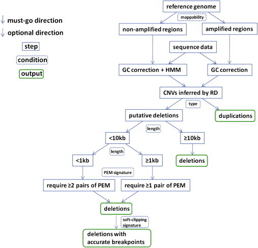
ERDS Flow Chart

Partition of the Reference Genome into Amplified and Nonamplified Regions

In NGS, short reads sequenced from repetitive regions can often be mapped to multiple locations equally well. The mrFAST²³ and mrsFAST²⁵ aligners can efficiently store all possible mapping locations of reads, making it possible to accurately predict the absolute copy numbers of regions. However, the resulting alignment data are not suitable for calling other kinds of variants, meaning that separate alignment would be required for calling SNVs and structural variants. We therefore sought to establish a framework to be able to accurately infer copy-number status even in SD regions by using data aligned by BWA, which randomly places a read to only one of the mappable locations by default. Instead of using a static predefined distinction between SD regions and unique genomic regions, however, we sought to divide the genome into regions that are distinguishable by BWA and those that are not. We identified such regions by taking each 1 kb segment of the reference genome and searching throughout the remainder of the genome for paralogous segments. Using simulated reads of length 100 bp, we partitioned the reference genome into two parts: amplified regions and nonamplified regions. To do this, we relied solely upon whether the sequence from a region was distinguishable by BWA. The amplified regions (regions not distinguishable by BWA) correspond to a subset of the UCSC SD regions (about one-third by genomic length) that have nearly identical paralogous regions (identity ≥ 0.99 in general). The reason to identify the amplified regions is to determine whether to call CNVs in a locus-specific manner or to calculate a genome-wide sum of copy numbers (absolute copy numbers) across all paralogous loci in amplified regions. CNVer¹⁶ has a similar step of partitioning the reference to avoid calling locus-specific copy numbers for paralogous loci.

Estimation of Expected RD

This step is essential to the accuracy of an RD-based method for both identifying and genotyping (determining the allelic state of) CNVs. For each sample, we calculated the RD for nonoverlapping sliding windows across the autosomes (200 bp was used in this study, but window size can be adjusted by the user). We averaged the mapping-quality scores of all bases within a window to produce an overall mapping-quality score for the window. We then grouped the windows with non-zero mapping-quality scores into bins with respect to the G + C percentage and estimated the expected RD of the diploid state in each G + C bin by using an expectation-maximization (EM) approach.²⁶

Initial Copy-Number Inference

For nonamplified regions, we applied a continuous paired HMM to detect CNVs by incorporating both RD data and SNV heterozygosity data. The emission probabilities were estimated with Poisson models, the transition probabilities were derived from the Baum-Welch algorithm, and the most-likely copy-number states for windows were inferred with the Viterbi algorithm.²⁷ At amplified regions, we summed up the RD of the windows for each set of indistinguishable regions identified and proceeded to the genotyping step (see below).

Refinement of Deletions

NGS data present multiple types of signatures that can be used for CNV detection. Although a method based on a single signature is conceptually simple, it is difficult for such a method to achieve both high sensitivity and a low FDR.¹⁵ To our knowledge, CNVer, Genome STRiP, and SV-Finder are the other tools that combine multiple signatures to detect CNVs, but the approaches implemented vary. In the ERDS framework, we integrated PEM and soft-clipping (SC) signatures²⁸ into the RD-based approach to filter possible false positives, confirm weak RD signals, and refine the breakpoints of putative deletions, as follows (also see Appendix A). (1) As the RD (or PEM)-based approach becomes less (or more) reliable for smaller deletions^16,17, we set a threshold of 10 kb above which all RD-predicted CNVs are accepted but below which additional PEM signatures are required for support. (2) The HMM approach probably misses weak signals that are several windows in length in a Markov chain. ERDS therefore scans through all of the uncalled regions to pick up the segments with RD ratios (observed RD to expected RD) that are smaller than a certain threshold and searches for supporting PEM signatures nearby to generate additional deletion calls. (3) For a putative deletion, whenever PEM or SC signatures are available, ERDS employs the signatures to refine the boundaries.

Genotyping

ERDS calculates the integer copy number of every region on the basis of the ratio of the observed RD to the expected RD. ERDS then outputs regions where the inferred copy number of the sequenced sample is different from the absolute copy number of the reference genome. Defined deletions and duplications in nonamplified regions are based on the assumption that the reference is diploid, whereas in amplified regions the type is determined relative to the absolute copy number of the reference genome for the aggregated set of regions.

PCR Validation and Sanger sequencing

We used the reference genome sequence (300 bp both 3′ and 5′ of the deletion) to design primers that flank the putative deletion. We then amplified each deletion in the test samples and ran them out on a 1% agarose gel to verify the size for each test sample in a given primer set.

We then used Sanger sequencing to sequence the PCR product of the deletion regions in each test sample (forward and reverse) and determined whether the deletion was in fact present. For an amplified deletion, we checked that its product size matched the expected size in those predicted to have and to lack the deletion. When the amplifications were of the correct sizes, we concluded that the sizes matched and that the sequencing confirmed the deletion. Otherwise, we concluded that the sizes did not match and that the sequencing could not detect a deletion.

Results

Here and throughout the paper, we consider a stringent 50% reciprocal overlap criterion to declare that two CNV calls are the same. We chose to use UCSC SD regions in the evaluations instead of the amplified regions (BWA-indistinguishable regions) derived from the ERDS algorithm because UCSC SD regions are publically available; thus, the evaluations could be performed without reference to ERDS, and the results of comparisons would not be unfavorable to other tools. Regions not overlapping SDs are termed unique regions. When 50% or more of a region is covered by SD regions cumulatively, we say that region is in SD regions. We focused our evaluations on CNVs in unique regions or SD regions; a small category of regions that were intermediate, modestly overlapping (50% or less) SD regions were not considered. Sources for all data sets are provided in the Web Resources.

Evaluation of the 1000GP Release Set in NA12878

One challenge in comparing CNV calling methods is that the true pattern of CNVs is difficult to accurately characterize in any genome.^3,17,29 It is therefore necessary to compare methods by using calls that are known to be only partially accurate. One important reference data set for making such comparisons is the 1000GP “release set” in Mills et al.¹⁵ We therefore first carried out a careful evaluation of this set of calls in sample NA12878 by using publicly available data, including alignment files, SNV files, and parents’ SV data (Web Resources).

Our evaluations of the 1000GP release set (Figure 2; Appendix B) were limited to all deletions that were both greater than 1 kb and in unique regions because these are considered easier to call than SD regions. To evaluate whether called deletions were likely to be real, we considered several key data points, as outlined in Appendix B. In particular, we considered whether a putative deletion was seen in the parents of the subject considered, what the RD ratio was, and critically, whether there were many heterozygous SNVs in the region of the putative deletion. Using these simple assessment approaches, we found that in the release set, the FDR was 8% (95/1197) for deletions larger than 1 kb, 38% (80/212) for deletions larger than 10 kb, and a very high 77% (44/57, Table S1 in the Supplemental Data available with this article online) for deletions larger than 100 kb (Table 1). A goal of the 1000GP was to create a release set with an FDR ≤ 10%.¹⁵ Our analysis showed, however, that the FDR is very unevenly distributed with respect to deletion size and that it is substantially higher for larger deletions. The high FDR for the largest deletions appears to be due to the dependence on PEM signatures, which become less reliable with increasing deletion sizes.^16,17

Figure 2.

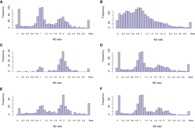
RD Assessment of Deletions in Unique Regions in the Release Set

RD ratios for regions were calculated as the ratio of the observed RD to the expected RD according to the G + C percentage. A ratio of 1.5 or smaller in unique regions suggests a deletion; confidence increases as the RD ratio decreases and the length of the region increases. Histograms of counts with respect to RD ratios were plotted for different categories with a bin width of 0.1. Different sizes are compared: (A) those larger than 1 kb (n = 1197) and (B) those smaller than 1 kb (n = 3385). For deletions larger than 1 kb, (C) those that failed the heterozygosity check (n = 163) and (D) those that passed the heterozygosity check (n = 1034) are shown. With regard to the deletion results in the parents, (E) those that are putative de novo (n = 378) and (F) those seen in one of the parents (n = 819) regardless of zygosity are shown.

Table 1.

Percentage of Deletions in the 1000GP Release Set that Failed According to Different Evaluation Approaches or Their Combinations

Category	Putative De Novo (A)	RD Ratio > 1.5 (B)	Violation of SNV Heterozygosity (C)	(A) & (B)	(A) & (C)	(B) & (C)	(A) & (B) & (C)
1 kb + (n = 1197)	32%	44%	14%	21%	9%	11%	8%
10 kb + (n = 212)	67%	66%	50%	54%	40%	45%	38%
100 kb + (n = 57)	93%	93%	84%	88%	79%	82%	77%

The analysis was limited to unique regions.

This evaluation suggests that the difficulty of detecting deletions accurately might have been underestimated and that there is considerable room for improvement of algorithms. This assessment also showed the importance of using RD information and SNV heterozygosity effectively in the inference of deletions. These two components are incorporated in the ERDS framework.

Evaluation of ERDS-Called Deletions

The comprehensive evaluations in Mills et al.¹⁵ demonstrated that Genome STRiP,¹⁸ which provided the lowest FDR of all the approaches included in that study, is the most sensitive tool for calling deletions in a low-coverage sample and that CNVnator³⁰ is the most sensitive tool for calling deletions in a high-coverage sample. We therefore sought to make direct comparisons of the performance of ERDS with Genome STRiP and CNVnator. No evaluations of the performance of Genome STRiP on high-coverage samples have been released.^15,18 Because Genome STRiP requires 20–30 genomes to reliably detect variants, we sequenced NA12878 at ∼40× in our center so that we could apply Genome STRiP (version 1.04.785) to NA12878 together with 24 other high-coverage samples sequenced in our center, and we also applied CNVnator (version 0.2.2) and ERDS (version 1.04) to call deletions (Table S2). We calculated the sensitivity of each approach in various size classes by using the GSD in Mills et al.¹⁵(Figure 3A). We broke down the data sets into size categories of <400 bp, 400 bp–1 kb, 1–10 kb, 10–100 kb and ≥100 kb. We needed to include the category of <400 bp to account for the abundant deletions caused by alu insertions in the reference genome, although apparently such deletions are underrepresented in the GSD.³¹ In general, Genome STRiP performed well in each length category, whereas CNVnator was most sensitive for large deletions. ERDS identified 70% of the deletions among a total of 3491 predictions (Table S3) and achieved a sensitivity 12% greater than that of the other two methods. ERDS remained the most sensitive method when we relaxed the overlapping criterion to a 1 bp overlap (Table S4). ERDS also performed well in SD regions (Table S5).

Figure 3.

Sensitivity Measurements for Different Approaches

The criterion of 50% reciprocal overlap was used (A) for calling deletions in NA12878 in the GSD from Mills et al. in different size classes and (B) for calling rare deletions in NA12878 with population frequencies of less than 1%, 2%, or 5% in Conrad et al.³

Because deletions in unique regions in the GSD should be more reliable than those in SD regions, we sought to evaluate the positive predictive value (PPV) of a call set only in unique regions, as defined by x/y, where x predictions in a call set overlapped with the GSD among y predictions in a given size range. As expected, Genome STRiP achieved the highest overall PPV (Table 2), consistent with its lower FDR.^15,18 ERDS showed PPVs almost identical to those of Genome STRiP in many categories. PPVs were nearly zero for all call sets for deletions smaller than 400 bp, mainly because small deletions were underrepresented in the GSD. If we restrict the evaluation to deletions larger than 400 bp, where the distribution of counts in GSD is presumably more accurate, then ERDS showed a PPV (0.28) slightly higher than Genome STRiP (0.26). It is also clear that the high sensitivity of CNVnator is achieved at the cost of a dramatically lower PPV (0.02).

Table 2.

PPVs for Deletions in Unique Regions in Different Size Categories

GSD as the Gold Standard
Category	<400 bp (n = 57)	400 bp-1kb (n = 79)	1–10 kb (n = 334)	10–100 kb (n = 56)	≥ 100 kb (n = 2)	Overall (n = 528)	≥ 400 bp (n = 471)
Genome STRiP	1|186|0.01	51|436|0.12	201|576|0.35	21|30|0.70	1|1|1.00	275|1229|0.22	274|1043|0.26
CNVnator	4|837|0.00	7|3464|0.00	194|7001|0.03	27|158|0.17	1|33|0.03	231|11493|0.02	228|10656|0.02
ERDS	13|1724|0.01	52|429|0.12	223|626|0.36	28|39|0.72	1|1|1.00	317|2819|0.11	304|1095|0.28

The Release Set as the Gold Standard
Category	<400 bp (n = 2772)	400 bp–1 kb (n = 613)	1–10 kb (n = 985)	10–100 kb (n = 155)	≥ 100 kb (n = 57)	Overall (n = 4582)
Genome STRiP	115|186|0.62	222|436|0.51	453|576|0.79	26|30|0.87	1|1|1.00	817|1229|0.66
CNVnator	221|837|0.26	183|3464|0.05	577|7001|0.08	37|158|0.23	2|33|0.06	1020|11493|0.09
ERDS	1173|1724|0.68	244|429|0.57	485|626|0.77	34|39|0.87	1|1|1.00	1937|2819|0.69

In the rows of categories, n represents the number of calls in the gold standard in a size range. The main cells are in the format of A|B|C, where A is the number of predictions that overlap the gold standard in a call set, B is the number of predictions in a particular size range in a call-set, and C is the PPV defined by A/B. Note that A is also an indication of sensitivity.

Because the GSD generally under-called variants, particularly small ones, we also calculated the PPV by using the release set as the gold standard by which to compare ERDS with Genome STRiP and CNVnator. In this comparison, ERDS showed the highest overall PPV and the highest PPVs in many categories, including the size category of <400 bp (Table 2). The overall PPV is 0.7, and this can be explained by the incompleteness of the release set.

Most examples of confirmed pathogenic CNVs are rare not only in population controls but also among the cases studied, consistent with the greater functional impact of rare CNVs.³ For this reason, it is of particular importance that any CNV calling method performs well for rare CNVs. In one of the largest CNV studies to date,³ CNV genotyping arrays were used for the detection of CNVs from 180 CEU samples, including NA12878. For the deletions observed in NA12878, we considered all those that were called in no more than 1%, 2%, or 5% of the considered samples, and we compared the performance of alternative calling methods among this critical set of rare deletions. We found that for all frequency cutoffs, ERDS had higher sensitivity than Genome STRiP and CNVnator: it called somewhere between 6% and 11% more deletions than the next-best method (Figure 3B).

To annotate the likely functional effects and potential clinical significance of a CNV, a method must not only detect the presence of a CNV but also accurately determine its breakpoints. ERDS achieves high breakpoint resolution as a result of the integration of PEM and SC signatures (Figure 4). We observed that ERDS provided 1,000 more deletions that exactly matched the breakpoints of deletions in the release set than did Genome STRiP or CNVnator. This is because the current versions of Genome STRiP and CNVnator do not incorporate SR or SC features in their approaches.

Figure 4.

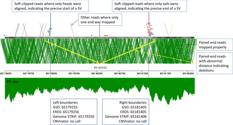
Breakpoint Resolutions of CNV Calls for a Deletion at chr10: 65179255–65181405 from the GSD.¹⁵

The top panel is plotted with SVviewer (Y.H., unpublished data) for displaying the aligned reads at region chr10: 65179255–65181405 along with 1 kb flanking regions at both sides. Both the PEM and SC signatures are integrated into the ERDS framework, making it possible to reach bp resolution in the breakpoint inference. The bottom panel is the RD plot for the same region. Although the RD was depleted in the middle, clear breakpoints were hard to indentify, in particular on the left-hand side. ERDS made a call at chr10: 65179256–65181405, which differed by 1 bp for the left breakpoint and matched the right breakpoint. Genome STRiP called the deletion at chr10: 65179250–65181408, which differed by 5 bp for the left breakpoint and 3 bp for the right breakpoint. CNVnator did not call this deletion.

Evaluation of ERDS-Called Duplications

Sample NA18507 is another widely studied sample.^20,23 We also sequenced this sample to ∼40× coverage and applied CNVnator and ERDS to call CNVs. When the duplication calls identified by a hybrid genotyping array²⁰ were used as the gold standard, ERDS showed slightly higher sensitivity for duplications than did CNVnator for both NA12878 and NA18507 (Table S6). Note that the overall sensitivity for duplications (approximately 50% in this evaluation) is lower than that for deletions (approximately 70% in the previous section) when NGS data are used, reflecting the increased difficulty in detecting duplications.

To further evaluate duplication calls from ERDS both for sensitivity and specificity, we sought to compare gene copy numbers derived from mrFAST and mrsFAST alignment results for sample NA18507 (Sudmant et al.,¹⁴ Alkan et al.,²³ and Can Alkan, personal communication). Because of the fundamentally different ways in which the aligners handle reads from repetitive regions, a direct comparison of copy-number calling in ERDS versus the mrFAST and mrsFAST framework is not possible, and an adjustment is required. For all genes, after this adjustment (Appendix C) to account for the difference caused by read lengths and aligners, the correlations between the adjusted ERDS result and mrFAST’s (Pearson correlation coefficient r = 0.66) or mrsFAST’s (r = 0.68) results approached the correlation between mrFAST’s and mrsFAST’s results (r = 0.84) (Figure S2).

Genotyping Accuracy

We sought to assess the accuracy of the genotyping results from ERDS. McCarroll et al. assigned copy numbers to samples on the basis of the ratio of the intensity values.²⁰ We used this data set to assess whether ERDS, having identified the type of a CNV (deletion versus duplication), can also predict the genotype (copy number). For samples NA12878 and NA18507, we found a high concordance rate for deletion calls but a lower concordance rate for duplications (Table S7). In rare cases, homozygous deletions were classified as heterozygous deletions, and vice versa. When restricted to unique regions, the concordance rates reached as high as 100% for both deletions and duplications in both samples.

Experimental Validations

The experimental validations were limited to deletions. Our comprehensive analysis on PPV had already computationally confirmed high confidence in the accuracy of ERDS calls.

Our strategy was to target the vulnerable calls, defined as the ERDS deletion calls that did not overlap with the release set, the GSD, or the Genome STRiP or CNVnator call sets in NA12878. Note that such vulnerable calls only comprised 27% (n = 936) of ERDS-called deletions. We further limited the validation to those deletions smaller than 2 kb (n = 698, 12% in SD regions) to increase the likelihood of a successful PCR assay. We have already determined that ERDS has higher PPV for larger deletions in general (Table 2). A subset of 23 calls (three in SD regions) were randomly chosen for performing PCR validations and Sanger sequencing from the 698 calls meeting the described inclusion criteria for validation (Table S8). For each of the vulnerable calls, we used one negative and one positive control sample. Primer design failed for two of the selected deletions. For the remaining 21 that were successfully analyzed, two had no amplification and two had incorrect product sizes. The other 17 (81%) have amplifications of the expected sizes, and Sanger sequencing confirmed the calls (Material and Methods).

We also performed validation by using TaqMan quantitative rtPCR assays. For this validation, we chose seven ERDS calls that were missed either by PennCNV³² or BreakDancer³³ in some of our samples. These deletions are larger than the deletions selected for PCR validation (median length is 20 kb). The TaqMan assays were commercially available on-demand assays through Applied Biosystems. For each selected deletion, we used the TaqMan assay targeting a gene within the deletion to ascertain the copy number in approximately 85 individuals, including the sample with the suspected CNV. The CNV was validated if the subject with the ERDS-called deletion was also found to harbor a deletion of the representative gene by the TaqMan assay. Two of the seven TaqMan assays failed to amplify the targeted DNA sufficiently to achieve accurate quantitative measurements and were therefore excluded from the analysis. Of the five reliable assays, four clearly confirmed the ERDS call. The deletion not validated by TaqMan is located in an SD region, where there is a paralogous sequence with 99.6% similarity. The TaqMan showed CN = 2 and thus no deletion. However, because the reference has four copies of this region and the TaqMan assay only showed CN = 2, we can infer that the ERDS’s deletion call is correct. Therefore, all deletions were validated when copy numbers were compared to those for the reference genome (Table S9).

Discussion

We have developed a tool called ERDS for detecting deletions and duplications. Importantly, ERDS uses the same alignment data (the BAM file) that are used for calling SNVs and INDELs, so that the computational burden remains manageable even for large studies. ERDS currently supports NCBI reference genome builds 36 and 37 and can be easily updated to future builds as they become available. Currently, on a PC with 8G memory, it can call CNVs for a sample with 40× coverage within 10 hr.

Using the same alignment file, we compared the performance of ERDS to two existing CNV-calling software tools, Genome STRiP and CNVnator, which appear to be the strongest alternative approaches available. The performance of each algorithm was affected by multiple complex factors, including coverage, library size, and read length. Overall, these direct comparisons showed that there are no CNV types for which ERDS performs worse with regard to high-coverage genomes. Genome STRiP, in particular, generally performs very well, but its performance clearly fell for the rarest deletions as compared to ERDS. However, ERDS performs at least as well as Genome STRiP for all other conditions as long as the genomes are sequenced to a coverage of at least 10×. For genomes sequenced at lower coverage, we recommend the use of Genome STRiP over ERDS (Table S10). We also note that ERDS analyzes one genome at a time, whereas Genome STRiP infers CNVs in population-scale sequencing data. It is possible that Genome STRiP offers some advantages in detecting structural variants that occur in multiple individuals in a data set, whereas ERDS will be superior in the detection of rare structural variants. We did not systematically evaluate the consequences of this difference in approach, however. Although Genome STRiP and CNVnator appear to be the strongest approaches currently available, ERDS does share some features with CNVer.²² We therefore also compared the performance of ERDS to CNVer and found that ERDS performs better for all classes of CNVs (Tables S6 and S11).

ERDS is also accurate at defining breakpoints for small deletions, and it reaches nucleotide resolution for many calls. Genotyping results of ERDS show excellent concordance with SNP array and FISH results (Table S12). Additionally, comprehensive computational evaluations and validations by PCR, Sanger sequencing, and TaqMan assays suggest that ERDS has a low FDR for deletions. Compared to that for deletions, the evaluation of called duplications was relatively weaker, because of both the lack of good reference and the technical difficulty of the experimental validations.

To compare ERDS with Genome STRiP and CNVnator, we sequenced two well-studied samples at high coverage, mainly because the evaluation of Genome STRiP on high-coverage samples was not publicly available and we needed to make the calls together with other samples sequenced at high coverage on the same sequencing platform. For the evaluation of the deletions in NA12878 in the release set in Mills et al., we only used publicly available data. For unique regions, in this evaluation we found that the larger a call, the less reliable it was. When applying these evaluations to Genome STRiP and ERDS in NA12878, we found that both approaches showed better accuracy than did the 1000GP release set (Table S13), in part because of the integration of multiple signatures into their calling frameworks. However, this improvement should also be acknowledged to be in part due to the improvement in the sequencing technology. The 1000GP itself will also have updated the calls with improved algorithms. Our evaluation of the 1000GP release set was limited to a single high-coverage sample; we did not attempt any evaluation of the low-coverage data.

Although many promising methods for CNV calling have emerged, many challenges remain. For example, certain large regions with extraordinary structural complexity¹⁴ confound current approaches. For example, duplications called by ERDS could be insertions at unknown genomic locations; identification of their precise locations therefore needs further work, possibly involving the incorporation of PEM information or other approaches. Sensitive detection of inversions and accurate inference of breakpoints of big deletions as well as duplications remain technically difficult. Improved tools that combine multiple signatures by starting from PEM signatures and SR features and then assessing the calls by using RD information to infer deletions accurately (essentially the reverse of the approach used here) are currently under development (Y.H., unpublished data). In theory, this approach can detect multiple types of complicated SVs, including insertions, translocations and inversions, across a wide range of sizes. Of note, sensitive and accurate detection of CNVs from exome sequence data are clearly more difficult, although tools such as CoNIFER³⁴ show significant progress.

In summary, ERDS is generally as good as any existing CNV-calling method and is superior in the key category of rare CNVs. When this approach is combined with the computational convenience of using the same alignment data as those used for calling other types of variants, ERDS appears to be one of the best all-around choices currently available for CNV calling in high-coverage samples, in particular for the detection of rare pathogenic CNVs in human disease.

Appendix A: Algorithm Development in ERDS

Identification of Amplified Regions in the Reference Genome

We simulated reads with lengths of 100 bp evenly across the reference genome and aligned them to the reference by using BWA with the option of mapping a read at up to 10,000 different locations. For each 1 kb region, if another region of similar length contributed reads of which more than half could be mapped to the current region, then that region was viewed as being paralogous to the current region. The sequences from these two regions usually had an overall identity that was greater than 0.99. The region and all of its paralogous regions were viewed as a set whose members could not be distinguished by BWA. We identified all paralogous regions throughout the reference genome and marked them as amplified regions.

The insertion size and read lengths will vary somewhat from sample to sample, and this will influence whether specific parts of the genome can or cannot be accurately aligned with BWA. Computational limitations restrict the ability to perform such an assessment specifically for each sample considered, and it is unlikely to be necessary. The aim of this step is simply to create a refined version of the UCSC SD regions, refined in the sense that we directly assess (approximately) which parts of the genome are and are not mappable by BWA. It is also important to appreciate that the purpose of identifying the amplified regions is to determine where to call locus-specific copy numbers or genome-wide summed copy numbers (absolute copy numbers). A further consideration is that if the amplified regions are identified in a sample-specific manner, then it is hard to compare the CNV results across sets of cases and controls in association studies.

G + C Correction

In the evaluation of the 1000GP release set, for each deletion we randomly found 20 other regions that have the same length and G + C percentage. We then determined the expected RD to be the median RD of these 20 regions. This analysis is completely independent of ERDS work.

In the ERDS framework, the RD for each 200 bp sliding window throughout the autosomes was calculated from the BAM file. Included was a noise-removing step that discarded loci in each window with extreme RD. Windows were grouped into 101 bins on the basis of their G + C content.

Our G + C estimation method is different from existing methods.^23,35 We sought to estimate the RD for the diploid state (normal state) in every bin. Note that a method in Yoon et al.³⁵ simply took the average RD of the whole bin. For a bin with T members, we adopted this approach if T < 200. We employed an EM algorithm²⁶ to estimate the expected RD when T ≥ 200. We assumed that the RD values in a bin were from a mixture of N Poisson distributions^13,16,36 corresponding to N copy-number states. Let O_t be the RD of the t-th windows and z_t be the latent variable, where z_t = i indicates that O_t belongs to the i-th copy-number state. Let the RD distribution from the i-th state be

$$p\left(O_t|z_t=i\right)\sim \frac{e^{-{\mathit{\lambda }}_i}{\mathit{\lambda }}_i^{O_t}}{\Gamma \left(O_t\right)},$$

where λ_i corresponds to the mean RD of the i-th copy-number state and Γ() is the Gamma function. We defined c_i = p(z_t = i) and deduced the following EM algorithm:

E step

$${\hat{c}}_{\iota }=\frac{\sum _{t=1}^T\frac{p\left(O_t,{\mathit{\lambda }}_i\right)C_i}{\sum _{j=1}^{5}p\left(O_t,{\mathit{\lambda }}_j\right)C_j}}{T}$$

and M step

$${\hat{\mathit{\lambda }}}_t=\frac{\sum _{t=1}^T\frac{p\left(O_t,{\mathit{\lambda }}_i\right)C_i}{\sum _{j=1}^{5}p\left(O_t,{\mathit{\lambda }}_j\right)C_j}{O}_t}{\sum _{t=1}^T\frac{p\left(O_t,{\mathit{\lambda }}_j\right)C_i}{\sum _{j=1}^{5}p\left(O_t,{\mathit{\lambda }}_j\right)C_j}},$$

where 0_t is the RD of the t-th member and c_i is the marginal probability of state i. After initial estimations of λ_i and c_i, ${\hat{\mathit{\lambda }}}_{\iota }$ and ${\hat{c}}_{\iota }$ were updated by this formula and eventually converged.

${\hat{\mathit{\lambda }}}_3\left(s\right)$ is considered to be the expected RD for the windows with G + C percentage s. Because sample sizes for other states are relatively small in comparison to that for the normal state, we estimated other values of ${\hat{\mathit{\lambda }}}_{\iota }$ simply by scaling

$$\widehat{{\mathit{\lambda }}_{\iota \ne 3}}=\frac{i}{2}\cdot {\hat{\mathit{\lambda }}}_3.$$

Paired HMM at Nonamplified Regions

HMMs²⁷ have been employed for calling CNVs from various types of data.^13,19,32 In this study, we viewed the RD of consecutive windows and heterozygosity information as a paired chain of observations, and we viewed the underlying copy numbers of windows as the hidden states. Considering that the RD can be any nonnegative rational number, we used a continuous paired HMM.

We defined n + 2 states representing CN = 0, …, n + 1. State n represents a collection of windows whose true copy number is at least n (n is suggested to be a number between 4 and 10; here, we used 6). We further created a “dummy” state n + 1, which represents windows at amplified regions or contig gaps. This state serves as a connector to make disconnected chains into a longer chain. Meanwhile, we kept the state from affecting the parameter estimation by assigning equal values to the transition probability for each state.

Emission Probabilities for RD

We estimated probability by using a Poisson distribution,

$$p\left(O_t|z_t=i\right)\sim \frac{e^{-{\hat{\mathit{\lambda }}}_t\left(s\right)}{\hat{\mathit{\lambda }}}_{\iota }{\left(s\right)}^{O_t}}{\Gamma \left(O_t\right)},$$

where s is the G + C percentage of the window under study and ${\hat{\mathit{\lambda }}}_{\iota }\left(s\right)$ was derived from the previous EM algorithm’s G + C correction.

Many noisy signals arose from repetitive regions that were not large enough to be characterized as amplified regions. The mapping qualities at those regions were usually low, and the RD signals were less reliable. We adjusted the emission probability for the t-th observation by multiplying by a weight

$$w_t=\frac{M{Q}_t}{M{Q}_{max}},$$

where MQ_t is the mapping quality of the current window and MQ_max is the maximum value used in the mapping-quality scores. In NA12878, about 92% of the alignable regions (the whole reference genome excluding N regions) have w_t ≥ 0.9. This is a heuristic and computationally inexpensive approach that ensures that the inference on one window with a poor mapping quality is based less upon its RD and more upon the RD of its neighboring regions with higher mapping qualities or upon a chain of windows with low mapping qualities that together can increase the signal.

Emission Probabilities for SNV Heterozygosity

Heterozygous SNVs were extracted from the variant file, which was either in SAMtools pileup format³⁷ or in vcf format.³⁸ We implemented a probabilistic approach to deal with possible errors of SNV calling or boundary issues. At the t-th window found to contain H_t > 0 heterozygous SNVs, we assigned a probability of $c_1\left(H_t\right)={10}^{-2-H_t}$ if the hidden state was a one-copy deletion and $c_0\left(H_t\right)={10}^{-3-H_t}$ if it was a two-copy deletion. The probabilities for other states were set to be equal to each other (and thus played no role in the decision-making process).

$$c_i\left(H_t\right)=\{\begin{array}{rr}\hfill {10}^{i-3-H_t,}& \hfill i=0,1\\ \hfill \frac{\left(1-c_0\left(H_t\right)-c_1\left(H_t\right)\right)}{10},& \hfill i\ge 2.\end{array}$$

We used these emission probabilities to penalize the heterozygosity at the regions of deletions. These parameters were fixed and free from updating in the Baum-Welch algorithm. More accurate modeling of the emission probabilities is difficult because of the noise carried in real data.

Transition Probabilities Matrix

We applied a modified Baum-Welch algorithm to update the transition probability matrix. The induction formula 20 in the forward procedure in a paper by Rabiner²⁷ becomes

$${\alpha }_{t+1}\left(i\right)=\left[\sum _{j=1}^N{\alpha }_t\left(i\right)a_{ij}\right]p\left(O_t,{\mathit{\lambda }}_j\right)c_j\left(H_t\right).$$

The induction formula 25 in the backward procedure becomes

$${\beta }_t\left(i\right)=\sum _{j=1}^N{a}_{ij}p\left(O_t,{\mathit{\lambda }}_j\right)c_j\left(H_t\right){\beta }_{t+1}\left(j\right).$$

Formula 40b becomes

$$\overline{a_{ij}}=\frac{\sum _{t=1,O_t\ne \text{null}}^{T-1}{\xi }_t\left(i,j\right)}{\sum _{t=1,O_t\ne \text{null}}^{T-1}{\gamma }_t\left(i\right)}.$$

We set the initial state probability to be the initial marginal probability of state i.

Paired Viterbi Algorithm and CNV Calling

We employed the Viterbi algorithm²⁷ to find the most likely chain of states (copy numbers). Because we had two sets of emission probabilities, we added an extra term coding for the second matrix to the initialization and recursion steps. Precisely, the formulas 32a and 33a in the Rabiner paper²⁷ were modified to be

$${\delta }_1\left(i\right)={\pi }_i{b}_i\left(O_1\right)c_i\left(H_1\right),1\le i\le N$$

and

$${\delta }_t\left(j\right)={\max }_{1\le i\le N}\left[{\delta }_{t-1}\left(i\right)a_{ij}\right]b_j\left(O_t\right)c_j\left(H_t\right),1\le j\le N,2\le t\le T,$$

where c_j(H_t) is the probability of seeing a case of SNVs H_t given state j.

The windows of the null or normal state were excluded. Consecutive windows with the same copy numbers were then merged.

Refinement for Deletions

• (1)For a putative deletion smaller than 10 kb, ERDS requires the support of the PEM signature (insert size > average library size + 3 SD). When the deletion is larger than 1 kb, ERDS requires one pair to support the deletion, and when it is smaller than 1 kb, ERDS requires two pairs. Users can adjust these parameters according to the coverage of a sample. A k-means clustering algorithm served to cluster the abnormally mapped paired-end reads and find the cluster that most supports the putative deletion. Suppose that p pairs of abnormal reads were found nearby and the requirement was q pairs; the algorithm would iteratively partition the pairs into k clusters, where k was defined as the least integer larger than p/q. Each pair was assigned to an initial cluster randomly. For each cluster, its mean is defined as (l_m, r_m), where l_m (or r_m) is the mean value of the left (or right) breakpoints of its members. In the next iteration, each pair was grouped to the nearest cluster. The distance from a pair with a left breakpoint l and a right breakpoint r to a cluster with mean (l_m, r_m) was defined as |l − l_m| + |r − r_m|. After a certain number of iterations (ten here), very few clusters, but at least one (Pigeonhole principle), would have members greater than or equal to q. Finally, for each cluster only the members with a distance that is less than the mean inner library size (defined as the mean library size − 2 × read length) were kept. The one with the highest product of the number of members in the cluster and the rate of the region defined by the cluster overlapping with the putative deletion region was then chosen to support the deletion. Here, k was set reasonably high so that the output cluster would be a true set of supporting signatures.
• (2)The HMM approach tends to miss weak (several-windows long) signals in a Markov chain mainly because of the penalty of the transition probabilities in an HMM. ERDS then scans through the whole-genome to pick up the segments with RD ratios (observed RD to expected RD) that are smaller than a threshold (for example, at 40× coverage, a window with RD ratio = 1.3 would be determined to represent a single copy by the Poisson model, whereas a window with RD ratio = 1.4 would be determined to be two copies) and checks whether there are PEM signatures overlapping this region (at least 3 pairs of PEM signatures are required) to generate additional deletion calls. Again, the parameters can be user specific.
• (3)For a putative deletion, when PEM or SC signatures are available, ERDS uses them to refine the breakpoints. The SC signature is denoted as “S” in the CIGAR column in a BAM file, indicating that a read has only been partially (the head or tail) mapped to the reference. A locus covered by two or more SC signatures within 200 bp of a breakpoint of a putative deletion is used to support that deletion.

In this step, many of the parameters were heuristic. Determination of the right set of parameters is always challenging because the true parameters are unclear or may not even exist. We selected parameters that were representative of different size categories, but users can optionally specify them in the command.

Genotyping

For the absolute copy number for each CNV ERDS called, we assigned an integer copy number on the basis of the ratio of the observed RD to the expected RD with respect to the G + C percentage. However, the copy number of an arbitrary region (gene region, FISH region, etc.) is the weighted mean value of the copy numbers when all deletions, normal regions, and duplication regions covering the region are taken into account. If we consider the reference genome as a sample, the absolute copy number of a region is estimated by the weighted mean value of nonamplified regions (copy number = 2) and amplified regions (copy number is twice the number of indistinguishable paralogous regions).

Appendix B: Evaluation of the 1000GP Release Set in NA12878

The release set contains deletions and insertions for more than 180 samples, including a majority of low-coverage samples and a few high-coverage samples.¹⁵ Here we only focused on the deletions in the high-coverage sample NA12878. Of note, Genome STRiP was not applied to this sample.^15,18

In this evaluation we limited our assessment to 1,197 deletions that were both larger than 1 kb and in unique regions (23% of a total of 5275 deletions) for higher confidence. First, we separated deletions in NA12878 into two groups: inherited (seen in either of the parents’ deletion results regardless of the zygosity) and putative de novo (others). Strikingly, 32% (n = 378) were found to be putative de novo. We can conclude that almost all of these putative de novo deletions were either false-positive calls in the child or false-negative calls in the parents, in part because of the multiple discrepancies both between the algorithms and between sequencing technologies.

We then assessed these deletions by using RD information from the alignment file originally used for inferring the deletions. For each deletion, we calculated its normalized RD ratio, that is, the observed RD adjusted by the expected RD according to the G + C percentage (Material and Methods), and multiplied by 2. A ratio of 1.5 or less in unique regions is suggestive of a deletion, and the smaller the RD ratio, the more confidently a deletion can be predicted. Similarly, the longer a region, the more reliable the RD ratio is. To reduce possible noise caused by boundary effects, we only counted the RD in the internal region; we excluded 10% on each side. We observed that 38% (454/1197) of the deletions in the release set had RD ratios larger than 1.5. A significant proportion of calls were centered at the peak RD ratio of 2 in the frequency histogram (Figure 2A), indicating no presence of deletions. More surprisingly, of those deletions larger than 10 kb and 100 kb in the release set, 66% (140/212) and 93% (53/57), respectively, had RD ratios greater than 1.5. We also calculated the RD ratio for those that were both smaller than 1 kb and in unique regions for a comparison. Although the correction for G + C bias is presumably less effective for small deletions, we were still able to find a peak at RD ratio = 1 and a long, thin tail toward larger ratios (Figure 2B).

A deletion in a unique region of an autosome means that, at most, one copy of the region is present in the genome; the deletion region should therefore not contain any heterozygous SNVs. SNV data from the 1000GP pilot data were used for this assessment. To account for possible boundary effects and potential SNV-calling errors in noisy real data, we only counted SNVs in the internal 80% region and considered a deletion to be supported if (1) it contained no more than two heterozygous SNVs or (2) no more than 20% of the SNVs were heterozygous. Considering that on average every 1 kb genomic region contains less than 1.2 SNVs,^39,40 many putative deletions regions would meet the first criterion even if no deletion were present. Therefore our heterozygosity check is a most-permissive possible assessment, and it probably only provides the lower bound of the FDR. Restricting deletions to those larger than 1 kb, 14% of deletions in the release set failed the heterozygosity check, and the majority of them had an RD ratio centered at 2 (Figure 2C), further indicating a false positive. As a comparison, two peaks representing homozygous and heterozygous deletions were clearly present in the plot for those that passed the heterozygosity check (Figure 2D). The failure rate for deletions larger than 10 kb (or 100 kb) is 50% (or 84%).

For the putative de novo deletions described above, 27.8% (n = 105) failed the heterozygosity check, and 58.2% (n = 220) had RD ratios greater than 1.5. In contrast, 7.1% (n = 58) of those inherited from parents failed the heterozygosity check, and 28.6% (n = 234) had RD ratios greater than 1.5 (Figures 2E and 2F).

It is reasonably safe to assume that a putative deletion called de novo and failing both the RD assessment and the heterozygosity check is incorrect. In this case (Table S1), the FDR in unique parts of the genome is 8% (95/1197) for deletions larger than 1 kb, 38% (80/212) for deletions larger than 10 kb, and 77% (44/57) for deletions larger than 100 kb (Table 1). Although the number of these false deletions is small because we focused on unique regions and applied the most stringent criteria in determining false calls, they made up approximately 22% of the whole call set in terms of genomic length and affected 13% of genes among those affected by the overall call set. This is because the FDR in the larger size category is higher.

One obvious question is why the FDR is so high for large deletions despite the careful attention to FDR of the contributing methods and the extensive use of experimental validation. Upon inspection, we found that approximately 96% (55/57) of those deletions larger than 100 kb were contributed by PEM or SR methods. This finding clearly explains part of the puzzle because the PEM and SR methods are known to be increasingly less reliable for large deletions, presumably as a result of the reduced accuracy of aligners in placing the pairs of short reads correctly over long distances.^16,17 The data for inferring CNVs in the 1000GP release set were from multiple centers with different sequencing platforms and included both single and paired-end reads generated with different insert sizes. These factors complicated the ability to make accurate calls.

Looking further at the false deletions larger than 1 kb, we found that each was validated by some approach, indicating that a careful assessment of the experimental validations is necessary for reducing errors.⁴¹ We checked the pass rate of different validation methods and found that deletions validated by comparative genomic hybridization (CGH) array approaches have the highest FDR, whereas deletions validated by polymerase chain reaction (PCR) and capture array approaches have nearly zero FDR (Figure S1). Upon further investigation, we found that the Nimblegen 2.1M array, chosen as the primary validation approach among CGH array approaches, was responsible for the majority of the false positives (in particular, 42/44 of false deletions larger than 100 kb). Interestingly, among all the CGH arrays evaluated by Pinto et al.,⁴¹ this array showed the lowest concordance rate between triplicate experiments and the highest FDR required to achieve a given sensitivity.

Appendix C: Evaluations of ERDS-Called Duplications

Although ERDS is based on BWA alignment, some of the philosophy behind mrFAST²³ and mrsFAST²⁵ has been integrated to allow improved estimation of the absolute copy number by summing the read depths from BWA-indistinuishable segments throughout the genome (Material and Methods). Because of the fundamental differences in how reads that can be mapped to multiple locations are considered, however, it is not meaningful to make direct comparisons between mrFAST- or mrsFAST-based copy-number results and BWA-based copy-number results. The simple reason for this is that whenever regions can be distinguished in the reference genome, ERDS will determine copy-number status relative to each distinguishable portion of segmental duplication regions, whereas mrFAST and mrsFAST will combine them. Therefore, as expected, agreement across all available 17,085 genes was initially low (Pearson correlation coefficient r = 0.33 for ERDS with mrFAST and r = 0.34 for ERDS with mrsFAST) (Figure S2A). Many factors contributed to the discrepancy between ERDS results and those of mrFAST and mrsFAST. For example, the alignment files used different sets of sequence data, and the length of our short reads was 101 bp, but in the previous studies all reads were trimmed to 36 bp by mrFAST and mrsFAST. It is likely that longer reads, even if originally distinguishable by an aligner, may become indistinguishable (even to the same aligner) after trimming. Thus, for the same gene, the count that BWA estimated (count_a) as present in the reference genome was not always identical to the count by mrFAST or mrsFAST (count_b).

We approximated count_a by using the absolute copy number of the reference genome in a given region (the genotyping step in the ERDS algorithm), and we approximated count_b by using publicly available CRG mappability data (Web Resources). The CRG mappability data show how many times every 36 bp read can be aligned to the reference genome with two or fewer mismatches. Repetitive regions and their flanking regions were masked, consistent with Alkan et al.²³ Intervals in SD (or non-SD) regions contributing reads that can be mapped to more than 100 (or 10) locations were also masked. In theory, count_a should equal count_b for every region because both measure how many times a region shows up in the reference genome. Using these approximations, we found that count_b is larger than count_a by 0.5 or more in 9% of the regions; less than 1% of the time, count_a is larger by 0.5 or more. The difference in the counts reflected the discrepancy caused by the different read lengths used. These results suggest that more paralogous regions were distinguished by BWA as a result of the longer read length we used.

For the purpose of evaluation, we corrected this difference by dividing the raw ERDS copy number of a gene by the approximated count_a and multiplied by the approximated count_b. This simple adjustment seems effective. For all genes, the correlations between the adjusted ERDS result and mrFAST’s (r = 0.66) or mrsFAST’s (r = 0.68) results approached the correlation between mrFAST and mrsFAST (r = 0.84). Approximately 85% of genes called as duplicated by mrFAST or mrsFAST were called by ERDS (Figure S2B); in SD regions, this number increased to 99%. This does not necessarily mean that ERDS was inaccurate, but rather it means that it was necessary to compensate for the bias introduced by aligners (among other factors).

Supplemental Data

Table S1. Putative Deletions that Occurred in NA12878 in the 1000GP Release Set and Failed Our Computational Assessment

These deletions are larger than 1 kb and occur in unique regions. They were called as de novo mutations and failed both the RD assessment and the heterozygosity check.

Web Resources

The URLs for data presented herein are as follows:

• The 1000GP release set, ftp://ftp-trace.ncbi.nih.gov/1000genomes/ftp/pilot_data/paper_data_sets/a_map_of_human_variation/trio/sv/trio.2010_10.deletions.sites.vcf.gz

• CRG mappability data, http://hgdownload.cse.ucsc.edu/goldPath/hg18/encodeDCC/wgEncodeMapability/

• The ERDS software, http://www.duke.edu/∼mz34/erds.htm

• The SNV data for sample NA12878, ftp://ftp-trace.ncbi.nih.gov/1000genomes/ftp/pilot_data/release/2010_07/trio/snps/CEU.trio.2010_03.genotypes.vcf.gz

References

- 1.Sebat J., Lakshmi B., Troge J., Alexander J., Young J., Lundin P., Månér S., Massa H., Walker M., Chi M. Large-scale copy number polymorphism in the human genome. Science. 2004;305:525–528. doi: 10.1126/science.1098918. [DOI] [PubMed] [Google Scholar]
- 2.Iafrate A.J., Feuk L., Rivera M.N., Listewnik M.L., Donahoe P.K., Qi Y., Scherer S.W., Lee C. Detection of large-scale variation in the human genome. Nat. Genet. 2004;36:949–951. doi: 10.1038/ng1416. [DOI] [PubMed] [Google Scholar]
- 3.Conrad D.F., Pinto D., Redon R., Feuk L., Gokcumen O., Zhang Y., Aerts J., Andrews T.D., Barnes C., Campbell P., Wellcome Trust Case Control Consortium Origins and functional impact of copy number variation in the human genome. Nature. 2010;464:704–712. doi: 10.1038/nature08516. [DOI] [PMC free article] [PubMed] [Google Scholar]
- 4.Cook E.H., Jr., Scherer S.W. Copy-number variations associated with neuropsychiatric conditions. Nature. 2008;455:919–923. doi: 10.1038/nature07458. [DOI] [PubMed] [Google Scholar]
- 5.Stefansson H., Rujescu D., Cichon S., Pietiläinen O.P., Ingason A., Steinberg S., Fossdal R., Sigurdsson E., Sigmundsson T., Buizer-Voskamp J.E., GROUP Large recurrent microdeletions associated with schizophrenia. Nature. 2008;455:232–236. doi: 10.1038/nature07229. [DOI] [PMC free article] [PubMed] [Google Scholar]
- 6.Stone J.L., O’Donovan M.C., Gurling H., Kirov G.K., Blackwood D.H., Corvin A., Craddock N.J., Gill M., Hultman C.M., Lichtenstein P., International Schizophrenia Consortium Rare chromosomal deletions and duplications increase risk of schizophrenia. Nature. 2008;455:237–241. doi: 10.1038/nature07239. [DOI] [PMC free article] [PubMed] [Google Scholar]
- 7.Glessner J.T., Wang K., Cai G., Korvatska O., Kim C.E., Wood S., Zhang H., Estes A., Brune C.W., Bradfield J.P. Autism genome-wide copy number variation reveals ubiquitin and neuronal genes. Nature. 2009;459:569–573. doi: 10.1038/nature07953. [DOI] [PMC free article] [PubMed] [Google Scholar]
- 8.de Kovel C.G., Trucks H., Helbig I., Mefford H.C., Baker C., Leu C., Kluck C., Muhle H., von Spiczak S., Ostertag P. Recurrent microdeletions at 15q11.2 and 16p13.11 predispose to idiopathic generalized epilepsies. Brain. 2010;133:23–32. doi: 10.1093/brain/awp262. [DOI] [PMC free article] [PubMed] [Google Scholar]
- 9.Heinzen E.L., Radtke R.A., Urban T.J., Cavalleri G.L., Depondt C., Need A.C., Walley N.M., Nicoletti P., Ge D., Catarino C.B. Rare deletions at 16p13.11 predispose to a diverse spectrum of sporadic epilepsy syndromes. Am. J. Hum. Genet. 2010;86:707–718. doi: 10.1016/j.ajhg.2010.03.018. [DOI] [PMC free article] [PubMed] [Google Scholar]
- 10.Pinto D., Pagnamenta A.T., Klei L., Anney R., Merico D., Regan R., Conroy J., Magalhaes T.R., Correia C., Abrahams B.S. Functional impact of global rare copy number variation in autism spectrum disorders. Nature. 2010;466:368–372. doi: 10.1038/nature09146. [DOI] [PMC free article] [PubMed] [Google Scholar]
- 11.Bochukova E.G., Huang N., Keogh J., Henning E., Purmann C., Blaszczyk K., Saeed S., Hamilton-Shield J., Clayton-Smith J., O’Rahilly S. Large, rare chromosomal deletions associated with severe early-onset obesity. Nature. 2010;463:666–670. doi: 10.1038/nature08689. [DOI] [PMC free article] [PubMed] [Google Scholar]
- 12.Walters R.G., Jacquemont S., Valsesia A., de Smith A.J., Martinet D., Andersson J., Falchi M., Chen F., Andrieux J., Lobbens S. A new highly penetrant form of obesity due to deletions on chromosome 16p11.2. Nature. 2010;463:671–675. doi: 10.1038/nature08727. [DOI] [PMC free article] [PubMed] [Google Scholar]
- 13.Bentley D.R., Balasubramanian S., Swerdlow H.P., Smith G.P., Milton J., Brown C.G., Hall K.P., Evers D.J., Barnes C.L., Bignell H.R. Accurate whole human genome sequencing using reversible terminator chemistry. Nature. 2008;456:53–59. doi: 10.1038/nature07517. [DOI] [PMC free article] [PubMed] [Google Scholar]
- 14.Sudmant P.H., Kitzman J.O., Antonacci F., Alkan C., Malig M., Tsalenko A., Sampas N., Bruhn L., Shendure J., Eichler E.E., 1000 Genomes Project Diversity of human copy number variation and multicopy genes. Science. 2010;330:641–646. doi: 10.1126/science.1197005. [DOI] [PMC free article] [PubMed] [Google Scholar]
- 15.Mills R.E., Walter K., Stewart C., Handsaker R.E., Chen K., Alkan C., Abyzov A., Yoon S.C., Ye K., Cheetham R.K., 1000 Genomes Project Mapping copy number variation by population-scale genome sequencing. Nature. 2011;470:59–65. doi: 10.1038/nature09708. [DOI] [PMC free article] [PubMed] [Google Scholar]
- 16.Medvedev P., Stanciu M., Brudno M. Computational methods for discovering structural variation with next-generation sequencing. Nat. Methods. 2009;6(11, Suppl):S13–S20. doi: 10.1038/nmeth.1374. [DOI] [PubMed] [Google Scholar]
- 17.Alkan C., Coe B.P., Eichler E.E. Genome structural variation discovery and genotyping. Nat. Rev. Genet. 2011;12:363–376. doi: 10.1038/nrg2958. [DOI] [PMC free article] [PubMed] [Google Scholar]
- 18.Handsaker R.E., Korn J.M., Nemesh J., McCarroll S.A. Discovery and genotyping of genome structural polymorphism by sequencing on a population scale. Nat. Genet. 2011;43:269–276. doi: 10.1038/ng.768. [DOI] [PMC free article] [PubMed] [Google Scholar]
- 19.Kidd J.M., Cooper G.M., Donahue W.F., Hayden H.S., Sampas N., Graves T., Hansen N., Teague B., Alkan C., Antonacci F. Mapping and sequencing of structural variation from eight human genomes. Nature. 2008;453:56–64. doi: 10.1038/nature06862. [DOI] [PMC free article] [PubMed] [Google Scholar]
- 20.McCarroll S.A., Kuruvilla F.G., Korn J.M., Cawley S., Nemesh J., Wysoker A., Shapero M.H., de Bakker P.I., Maller J.B., Kirby A. Integrated detection and population-genetic analysis of SNPs and copy number variation. Nat. Genet. 2008;40:1166–1174. doi: 10.1038/ng.238. [DOI] [PubMed] [Google Scholar]
- 21.Mills R.E., Luttig C.T., Larkins C.E., Beauchamp A., Tsui C., Pittard W.S., Devine S.E. An initial map of insertion and deletion (INDEL) variation in the human genome. Genome Res. 2006;16:1182–1190. doi: 10.1101/gr.4565806. [DOI] [PMC free article] [PubMed] [Google Scholar]
- 22.Medvedev P., Fiume M., Dzamba M., Smith T., Brudno M. Detecting copy number variation with mated short reads. Genome Res. 2010;20:1613–1622. doi: 10.1101/gr.106344.110. [DOI] [PMC free article] [PubMed] [Google Scholar]
- 23.Alkan C., Kidd J.M., Marques-Bonet T., Aksay G., Antonacci F., Hormozdiari F., Kitzman J.O., Baker C., Malig M., Mutlu O. Personalized copy number and segmental duplication maps using next-generation sequencing. Nat. Genet. 2009;41:1061–1067. doi: 10.1038/ng.437. [DOI] [PMC free article] [PubMed] [Google Scholar]
- 24.Li H., Durbin R. Fast and accurate short read alignment with Burrows-Wheeler transform. Bioinformatics. 2009;25:1754–1760. doi: 10.1093/bioinformatics/btp324. [DOI] [PMC free article] [PubMed] [Google Scholar]
- 25.Hach F., Hormozdiari F., Alkan C., Hormozdiari F., Birol I., Eichler E.E., Sahinalp S.C. mrsFAST: a cache-oblivious algorithm for short-read mapping. Nat. Methods. 2010;7:576–577. doi: 10.1038/nmeth0810-576. [DOI] [PMC free article] [PubMed] [Google Scholar]
- 26.Dempster A.P., Laird N.M., Rubin D.B. Maximum Likelihood from Incomplete Data via the EM Algorithm. J. R. Stat. Soc., B. 1977;39:1–38. [Google Scholar]
- 27.Rabiner L.R. A tutorial on Hidden Markov Models and selected applications in speech recognition. Proc. IEEE. 1989;77:257–286. [Google Scholar]
- 28.Wang J., Mullighan C.G., Easton J., Roberts S., Heatley S.L., Ma J., Rusch M.C., Chen K., Harris C.C., Ding L. CREST maps somatic structural variation in cancer genomes with base-pair resolution. Nat. Methods. 2011;8:652–654. doi: 10.1038/nmeth.1628. [DOI] [PMC free article] [PubMed] [Google Scholar]
- 29.Pang A.W., MacDonald J.R., Pinto D., Wei J., Rafiq M.A., Conrad D.F., Park H., Hurles M.E., Lee C., Venter J.C. Towards a comprehensive structural variation map of an individual human genome. Genome Biol. 2010;11:R52. doi: 10.1186/gb-2010-11-5-r52. [DOI] [PMC free article] [PubMed] [Google Scholar]
- 30.Abyzov A., Urban A.E., Snyder M., Gerstein M. CNVnator: an approach to discover, genotype, and characterize typical and atypical CNVs from family and population genome sequencing. Genome Res. 2011;21:974–984. doi: 10.1101/gr.114876.110. [DOI] [PMC free article] [PubMed] [Google Scholar]
- 31.Stewart C., Kural D., Strömberg M.P., Walker J.A., Konkel M.K., Stütz A.M., Urban A.E., Grubert F., Lam H.Y., Lee W.P., 1000 Genomes Project A comprehensive map of mobile element insertion polymorphisms in humans. PLoS Genet. 2011;7:e1002236. doi: 10.1371/journal.pgen.1002236. [DOI] [PMC free article] [PubMed] [Google Scholar]
- 32.Wang K., Li M., Hadley D., Liu R., Glessner J., Grant S.F., Hakonarson H., Bucan M. PennCNV: an integrated hidden Markov model designed for high-resolution copy number variation detection in whole-genome SNP genotyping data. Genome Res. 2007;17:1665–1674. doi: 10.1101/gr.6861907. [DOI] [PMC free article] [PubMed] [Google Scholar]
- 33.Chen K., Wallis J.W., McLellan M.D., Larson D.E., Kalicki J.M., Pohl C.S., McGrath S.D., Wendl M.C., Zhang Q., Locke D.P. BreakDancer: an algorithm for high-resolution mapping of genomic structural variation. Nat. Methods. 2009;6:677–681. doi: 10.1038/nmeth.1363. [DOI] [PMC free article] [PubMed] [Google Scholar]
- 34.Krumm N., Sudmant P.H., Ko A., O’Roak B.J., Malig M., Coe B.P., Quinlan A.R., Nickerson D.A., Eichler E.E., NHLBI Exome Sequencing Project Copy number variation detection and genotyping from exome sequence data. Genome Res. 2012;22:1525–1532. doi: 10.1101/gr.138115.112. [DOI] [PMC free article] [PubMed] [Google Scholar]
- 35.Yoon S., Xuan Z., Makarov V., Ye K., Sebat J. Sensitive and accurate detection of copy number variants using read depth of coverage. Genome Res. 2009;19:1586–1592. doi: 10.1101/gr.092981.109. [DOI] [PMC free article] [PubMed] [Google Scholar]
- 36.Lander E.S., Waterman M.S. Genomic mapping by fingerprinting random clones: a mathematical analysis. Genomics. 1988;2:231–239. doi: 10.1016/0888-7543(88)90007-9. [DOI] [PubMed] [Google Scholar]
- 37.Li H., Handsaker B., Wysoker A., Fennell T., Ruan J., Homer N., Marth G., Abecasis G., Durbin R., 1000 Genome Project Data Processing Subgroup The Sequence Alignment/Map format and SAMtools. Bioinformatics. 2009;25:2078–2079. doi: 10.1093/bioinformatics/btp352. [DOI] [PMC free article] [PubMed] [Google Scholar]
- 38.Danecek P., Auton A., Abecasis G., Albers C.A., Banks E., DePristo M.A., Handsaker R.E., Lunter G., Marth G.T., Sherry S.T., 1000 Genomes Project Analysis Group The variant call format and VCFtools. Bioinformatics. 2011;27:2156–2158. doi: 10.1093/bioinformatics/btr330. [DOI] [PMC free article] [PubMed] [Google Scholar]
- 39.1000 Genomes Project Consortium A map of human genome variation from population-scale sequencing. Nature. 2010;467:1061–1073. doi: 10.1038/nature09534. [DOI] [PMC free article] [PubMed] [Google Scholar]
- 40.Pelak K., Shianna K.V., Ge D., Maia J.M., Zhu M., Smith J.P., Cirulli E.T., Fellay J., Dickson S.P., Gumbs C.E. The characterization of twenty sequenced human genomes. PLoS Genet. 2010;6:e1001111. doi: 10.1371/journal.pgen.1001111. [DOI] [PMC free article] [PubMed] [Google Scholar]
- 41.Pinto D., Darvishi K., Shi X., Rajan D., Rigler D., Fitzgerald T., Lionel A.C., Thiruvahindrapuram B., Macdonald J.R., Mills R. Comprehensive assessment of array-based platforms and calling algorithms for detection of copy number variants. Nat. Biotechnol. 2011;29:512–520. doi: 10.1038/nbt.1852. [DOI] [PMC free article] [PubMed] [Google Scholar]
Associated Data
This section collects any data citations, data availability statements, or supplementary materials included in this article.
Supplementary Materials