On-the-fly free energy parameterization via temperature accelerated molecular dynamics

Abstract

We discuss a method for parametric calculation of free energy functions in arbitrary collective variables using molecular simulations. The method uses a variant of temperature accelerated molecular dynamics to evolve on-the-fly the parameters of the free energy function to their optimum values by minimization of a cumulative gradient error. We illustrate how the method performs using simple examples and discuss its application in the derivation of effective pairwise potentials for multiscale molecular simulations.

1. Introduction

A common task in molecular simulations is the estimation of a free energy G(z) in some collective variables (CV’s) θ(x):

$$G(\mathit{z})=-k_{B}Tln\langle \delta [\mathit{\theta }(\mathit{x})-\mathit{z}]\rangle$$ (1)

Here, z is some target value of the CV’s, and 〈·〉 implies an ensemble average over configurational space. The Dirac delta function picks out only those configurations for which the CV θ(x) is z. The free energy is useful because it permits one to measure the relative importance of regions of CV space, which ultimately leads to the prediction of metastable equilibrium states in this space: these are the regions around the local minima in G. A perfectly ergodic, infinitely long MD trajectory would spend much more time in these regions than it would in the intervening spaces. In all too many actual cases, MD trajectories remain close to only one metastable state (the one closest to the initial state of the simulation) and only very rarely, if ever, visit others. Once one has invoked CV’s, one realizes that MD simulations often fail to overcome free energy barriers. Moreover, these intervening regions of CV-space can be examined for low-free-energy routes that join states, and these routes are often associated with reaction mechanisms that convert one state to another.

Free energy methods such as thermodynamic integration [1], umbrella sampling/histogram reweighting [2], and non-equilibrium work methods [3, 4], and metadynamics [5] are most often employed to compute free energies in relatively low-dimensional spaces. These methods all differ in detail, but they all in essence force a system to explore its CV space as uniformly as possible, and at each location in CV-space (subject to some resolution of discretization), to sample configurations. That is, they are all more or less sophisticated ways of binning configurations into CV histograms. Because of this, these methods are somewhat limited in that they rapidly become inefficient when the dimensionality of CV space is large (more than a handful of independent CV’s).

More recently, the single-sweep method has been shown useful for computation of free energy in a few CV’s, [6] and the CV-version of string method continues to find application in computing pathways of minimal free energy through relatively high-dimensional CV spaces. [7, 8] The exploration of relevant but difficult-to-access regions in high-dimensional CV spaces (which is a requisite part of single sweep and indeed any free energy method) is possible using temperature-accelerated MD (TAMD). [9, 10] TAMD augments the set of independent variables with auxiliary variables that are tethered to the CV’s and evolve in lockstep with the atomic variables. A particular feature of TAMD worth mentioning here is that it uses effective time-averaging of restraining forces to compute gradients in free energy on-the-fly which govern evolution of the CVs: in other words, TAMD reports the instantaneous value of the mean force, a fact that we will exploit here. It is also worth mentioning that TAMD is essentially identical to the driven adiabatic free energy dynamics approach (d-AFED), [11] which is itself based on adiabatic free energy dynamics (AFED) [12] in which CV’s are evolved directly by their own equations of motion rather than by tethering to auxiliary variables.

A type of free energy calculation that has received particular attention is the derivation of effective pair potentials for describing how molecules interact at some level of resolution coarser than the atomic level. Several approaches for deriving “systematically coarse-grained” effective pair potentials from fine-grained simulations have gained popularity, including iterative-Boltzmann inversion, [13, 14] force-matching, [15{17] and minimization of relative entropy. [18] These approaches all have advantages and disadvantages, but they have in common the fact that ensemble averaging is performed at a particular thermodynamic state point using all-atom (or fine-grained) molecular simulation to accumulate statistics in the coarse-grained variables that constitute the arguments of the effective pairwise potentials. This means that such methods are practically limited in their accuracy by the sampling of the all-atom system. It might therefore be advantageous if some kind of enhanced-sampling method, such as TAMD, could be called upon for such derivations in the hopes of avoiding sampling issues arising, for example, from metastabilities or hidden barriers.

Here we propose an approach in which a TAMD-related method can be used to determine the parameters of an assumed analytical free energy function whose primary variables are functions of CV’s. That is, we propose a adaptation of TAMD which can in principle determine free energy of a high-dimensional CV space. We have dubbed this method temperature accelerated MD/on-the-fly parameterization (TAMD/OTFP). We present the theoretical framework of TAMD/OFTP in the next section, followed by examples of its application both to a simple 1- and 2-D systems and to high-dimensional molecular fluids, ultimately demonstrating how it can be used to derive effective pair-wise potentials for single-site water. We conclude with a discussion of possibilities for broader application of TAMD/OTFP.

2. Temperature Accelerated MD On-the-Fly Parameterization

The general structure of the TAMD/OTFP method can be introduced as follows. Suppose that we are interested in computing the free energy G(z) of the collective variables θ(x), defined as in Eq. 1. Suppose also that we know (or think we do) the functional form of G(z) up to some unknown parameters λ, i.e.

$$G(\mathit{z})=G(\mathit{z},{\mathit{\lambda }}^{\ast })$$ (2)

for some λ^* unknown to us – our aim will be to determine them. To this end, we start with the TAMD system of equations [9]

$$\begin{array}{l}{M}_x\ddot{\mathit{x}}=-{\nabla }_{x}V[\mathit{x}(t)]-k[\mathit{\theta }[\mathit{x}(t)]-\mathit{z}(t)]\nabla \mathit{\theta }[\mathit{x}(t)]+\text{bath}\text{at}{\beta }^{-1}\\ M_z\ddot{\mathit{z}}=k[\mathit{\theta }[\mathit{x}(t)]-\mathit{z}(t)]+\text{bath}\text{at}{\overline{\beta }}^{-1}\end{array}$$ (3)

Here, β = 1/k_BT, where T is the physical temperature of the system, and β̄ = 1/k_BT̄, where T̄ > T is an artificial temperature used to accelerate the sampling. A central feature of TAMD is that, if the (artificial) masses M_z of the CVs z are taken much larger than the masses M_x of the physical variables x so that the former evolve slower than the latter, the forces acting on z self-average to negative gradients of the free energy at the physical temperature T, i.e.

$$k[\mathit{\theta }[\mathit{x}(t)]-\mathit{z}(t)]\approx -{\nabla }_{z}G(\mathit{z}(t))$$ (4)

Here we use property to determine on-the-fly the optimal value of the parameters λ given the available information gathered along the solution of Eq. 3 up to the current time t via minimization of the following gradient-error measure:

$$E(\mathit{\lambda },t)=\frac{1}{2t}{\int }_0^t{\mid {\nabla }_{z}G[\mathit{z}(s),\mathit{\lambda }]+k[\theta (\mathit{x}(s)-\mathit{z}(s)]\mid }^{2}ds,$$ (5)

As time t progresses, the minimizer of this functional will converge to the optimal value λ^*. In practice, the TAMD can be stopped when such convergence has been achieved.

Note that, while the functional (5) uses the TAMD trajectory, the minimization of this functional does not feedback on this simulation, i.e. it can be done independently. Depending on the functional form of the free energy in (2), different strategies can be used for the minimization of (5). Here, we will restrict ourselves to functional forms of G which are linear in the parameters λ. In this case, the minization of (5) reduces to the solution of a set of linear equations in λ that is obtained by setting the derivatives of E with respect to any λ_j to zero and may be expressed generally as

$$\mathit{A}(t)\mathit{\lambda }(t)=\mathit{b}(t)$$ (6)

where the elements of the matrix A(t) and vector b(t) are determined from the parameterless parts of G, as will be illustrated in the following four examples.

Before proceeding to the examples, we remark that it is possible to replace the TAMD sysem of equations (3) by the system

$$\begin{array}{l}{M}_x\ddot{\mathit{x}}=-{\nabla }_{x}V[\mathit{x}(t)]-k[\mathit{\theta }[\mathit{x}(t)]-\mathit{z}(t)]\nabla \mathit{\theta }[\mathit{x}(t)]+\text{bath}\text{at}{\beta }^{-1}\\ M_z\ddot{\mathit{z}}=-{\nabla }_{z}G[\mathit{z}(t),\mathit{\lambda }(t)]+\text{bath}\text{at}{\overline{\beta }}^{-1}\end{array}$$ (7)

in which the forces on z arise from the analytical free energy G evaluated using instantaneous values of the parameters λ obtained by minimizing (5). With such modification, TAMD/OTFP fits the framework of the heterogeneous multiscale method (HMM), [19, 20] which confers it the advantage over the original TAMD that more sophisticated schemes can be used to integrate the equation of motion for the CVs by exploiting the known functional form of the free energy. Though none of the examples in this paper fits this criterion, we nevertheless show in one of the four examples (#3) that the approach of using analytical forces to update z is equally effecacious at converging λ as using the TAMD forces.

3. Example 1: A Simple 1D Two-Well Potential

A simple example can serve to illustrate how the TAMD/OTFP method works. Suppose that x is one-dimensional, and is subject to the following potential:

$$V(x)=\frac{1}{4}{(1-x^2)}^2$$ (8)

and let us simply take θ(x) = x, so that G(z) = V (z). Let us also assume that our parameterized version of G is

$$G(z,\lambda )=-\frac{\lambda }{2}{z}^2+\frac{1}{4}{z}^4,$$ (9)

which, up to an irrelevant constant, is indeed consistent with the true G(z) for λ^* = 1. The overdamped limit of the TAMD equations for this system can be written

$$\begin{array}{l}{\gamma }_x\stackrel{.}{x}=x-x^3-k(x-z)+\sqrt{2{\beta }^{-1}{\gamma }_x}{\eta }_x\\ {\gamma }_z\stackrel{.}{z}=k(x-z)+\sqrt{2{\overline{\beta }}^{-1}{\gamma }_z}{\eta }_z.\end{array}$$ (10)

Using the definition of the error shown in (5), we may at any time t in the TAMD simulation compute a best-estimate of the parameter λ using

$$\lambda (t)=\frac{b(t)}{A(t)}$$ (11)

representing a scalar, inverted form of (6), where

$$A(t)=\frac{1}{t}{\int }_0^t{z}^2(s)ds,b(t)=\frac{1}{t}{\int }_0^t\{k[z(s)-x(s)]-z^3(s)\}z(s)ds$$ (12)

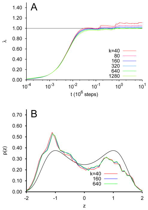
Explicit numerical integration of these equations of motion was used to explore the convergence behavior of λ to 1. First, in Fig. 1A, we show λ vs t for the case of γ_x = 1, γ_z = 1000, β⁻¹ = 0.02 and β̄⁻¹ = 0.6 (for comparison the barrier between the minima of (8) is 0.25), for various values of k between 40 and 1280. The time step of the integration was 1×10⁻² for k=40. We observe that λ indeed converges quickly (on the time scale at which transition between the wells ocurs at the physical temperature). We also observe the trend that the converged value for λ becomes more accurate as k is increased. Fig. 1B shows the histogram of the observed value of z binned from the entire trajectories for selected values of k. It can be seen that the full domain of z is sampled, but that the sampling alone does not provide a perfectly accurate recapitulation of the free energy.

FIG. 1.

TAMD/OTFP for the system of Eq. 10 at β̄⁻¹ = 0.6. (A) Convergence of λ of Eq. 9 to λ* via integration of Eq. 10 for various values of k. (B) Probability distribution of z for selected values of k, with the Boltzmann distribution for G(z).

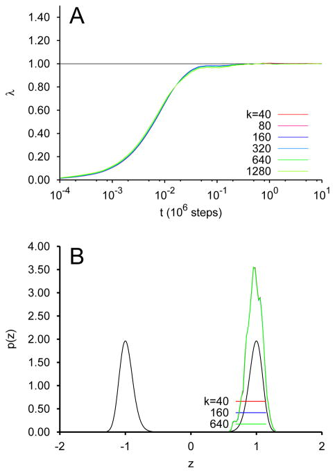
This situation is contrasted by the data in Fig. 2A and B, which correspond to the same integrations except with the fictitious temperature β̄⁻¹ = 0.02. Interestingly, λ again converges well to 1 (Fig. 2A), but Fig. 2B illustrates that only the right-hand well is sampled. Although the evolution only sampled the region around the local minimum and never crossed the barrier, that still provided enough information to converge λ to 1 for the given functional form imposed. This serves to illustrate the risk of “overinterpretation” by attempting to fit a functional form which is inherently symmetric.

FIG. 2.

TAMD/OTFP for the system of Eq. 10 at β̄⁻¹ = 0.02. (A) Convergence of λ of Eq. 9 to λ* via integration of Eq. 10 for various values of k. (B) Probability distribution of z for selected values of k, with the Boltzmann distribution for G(z).

4. Example 2: A 2D Potential and 1D CV

In the previous example, we took θ(x) = x as a CV definition on a 1D potential (meaning the “free” energy is really the potential energy) solely to show that the TAMD/OTFP algorithm correctly parameterizes a potential energy, which it must minimally be able to do before it can be shown to correctly parameterize a free energy. In this second simple example, we show that TAMD/OTFP correctly parameterizes a 1D free energy on a 2D potential. Consider the potential energy

$$V(x,y)=exp(2a{sin}^{2}x)\frac{1}{2}{y}^2$$ (13)

Let us take θ(x, y) = x, in which case the free energy (to within an irrelevant constant) is of the form

$$G(z;\lambda )=\frac{1}{\beta }\lambda {sin}^{2}z.$$ (14)

Clearly, λ = a for the potential defined in Eq. 13 with θ(x, y) = x. We show now that the TAMD/OTFP scheme converges arbitrary initial λ to a. Applying the overdamped limit of the TAMD/OTFP scheme to the present example yields

$$\begin{array}{l}{\gamma }_x\stackrel{.}{x}=-2y^{2}exp(2\mathit{a}{sin}^{2}x)\mathit{a}sin\mathit{x}cos\mathit{x}-k(x-z)+\sqrt{2{\beta }^{-1}{\gamma }_x}{\eta }_x\\ {\gamma }_y\stackrel{.}{y}=-yexp(2a{sin}^{2}x)+\sqrt{2{\beta }^{-1}{\gamma }_y}{\eta }_y\\ {\gamma }_z\stackrel{.}{z}=k(x-z)+\sqrt{2{\overline{\beta }}^{-1}{\gamma }_z}{\eta }_z,\end{array}$$ (15)

and

$$\lambda (t)=\frac{b(t)}{A(t)}$$ (16)

where

$$\begin{array}{l}A(t)=\frac{1}{t}{\int }_0^t\frac{4}{\beta }sinz(s){cos}^{2}z(s)ds,\\ b(t)=-\frac{1}{t}{\int }_0^t\frac{2}{\beta }sinz(s)cosz(s)k[z(s)-x(s)]ds,\end{array}$$ (17)

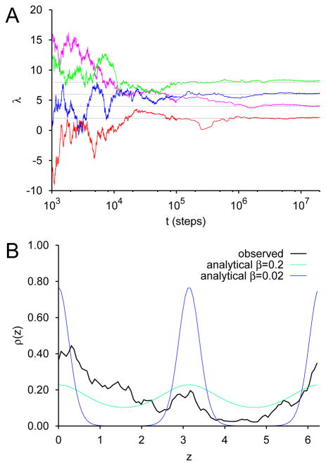
These equations were integrated for a = 2.0, 4.0, 6.0 and 8.0, using a semi-implicit numerical scheme. Results are shown in Fig. 3. Here we have taken a timestep of 0.01, a coupling constant k = 1,000, γ_x = γ_y = 1, γ_z = 1, 000, β⁻¹ = 0.02 and β̄⁻¹ = 0.2. We observe that λ coverges to a for all values of a considered, and that convergence is achieved at about 10⁶ steps in all cases (Fig. 3A). Thus TAMD/OTFP can correctly parameterize a true free energy; i.e., one that arises from dimensional reduction. Fig. 3B shows for a representative 2×10⁷-step integration (a = 8) the probability distribution ρ(z) observed empirically for z, as well as the analytical free energy G(z). Note that, although TAMD induces z to traverse its entire domain [−π, π], the histogram of visited values of z is a fairly poor representation of the true analytical probability distribution z must obey, yet the parameterization of G(z) has converged. This indicates that in the present example it is more efficient to determine the parameters of the free energy of a known functional form than it is to determine the free energy by inversion of a histogram.

FIG. 3.

TAMD/OTFP for the system of Eq. 15 with a = 2, 4, 6, and 8, and β̄⁻¹ = 0.2. (A) Convergence of λ of Eq. 14 to a via integration of Eq. 15 for various values of a. (B) Probability distribution of z for a representative integration with a = 8, with the Boltzmann distributions for G(z) at both β⁻¹ = 0.02 and 0.2.

5. Examples 3 and 4: Coarse-grained effective pairwise potentials

We show in this section that, with a suitable choice for a flexible functional form, we can use TAMD/OTFP to construct effective pair potentials between centers of mass of a coarse-grained system. To start, we represent our unparameterized free energy as a sum of effective pair potentials:

$$G(\mathit{z};\mathit{\lambda })=\sum _{i<j}g(\mid {\mathit{z}}_i-{\mathit{z}}_j\mid ;\mathit{\lambda })$$ (18)

Here, z ∈ {z_iα; i = 1 … N; α = x, y, z}, are the cartesian coordinates of molecular centers-of-mass. We case that pair potential as a linear expansion in basis functions:

$$g(z;\mathit{\lambda })=\sum _k{\lambda }_k{\phi }_k(z)$$ (19)

This of course means that the overall free energy, as a pairwise sum, is indeed linear in the parameters λ. At any time t in a TAMD/OTFP integration, the error defined in Eq. 5 for this choice can therefore be cast as (neglecting terms that are independent of λ and therefore do not affect the minimizer)

$$E(\mathit{\lambda },t)=\sum _m{\lambda }_m\frac{1}{t}{\int }_0^t\sum _{i\alpha }k[{\theta }_{i\alpha }(\mathit{x}(s))-z_{i\alpha }(s)]\left(\sum _{j\ne i}\frac{z_{ij\alpha }}{z_{ij}}\frac{\partial {\phi }_m}{\partial z_{ij}}\right)ds$$ (20)

$$+\frac{1}{2}\sum _{mn}{\lambda }_m{\lambda }_n\frac{1}{t}{\int }_0^t\sum _{i\alpha }\left(\sum _{j\ne i}\frac{z_{ij\alpha }}{z_{ij}}\frac{\partial {\phi }_m}{\partial z_{ij}}\right)\left(\sum _{j\ne i}\frac{z_{ij\alpha }}{z_{ij}}\frac{\partial {\phi }_n}{\partial z_{ij}}\right)ds$$ (21)

$$\equiv -\sum _m{\lambda }_m{b}_m(t)+\frac{1}{2}\sum _{mn}{\lambda }_m{\lambda }_n{A}_{mn}(t)$$ (22)

which defines the elements of the matrix A(t) and the vector b(t) in Eq. (6) for the optimal λ at time t.

Although any reasonable choice for the basis functions is possible, for simplicity we use standard linear chapeau functions:

$${\phi }_k(z)=\{\begin{array}{ll}\frac{1}{\mathrm{\Delta }z}[z-(k-1)\mathrm{\Delta }z]\hfill & \text{if}(k-1)\mathrm{\Delta }z<z<k\mathrm{\Delta }z,\text{and}\hfill \\ 1-\frac{1}{\mathrm{\Delta }z}[z-k\mathrm{\Delta }z]\hfill & \text{if}k\mathrm{\Delta }z<z<(k+1)\mathrm{\Delta }z,\text{and}\hfill \\ 0\hfill & \text{otherwise}.\hfill \end{array}$$ (23)

where we take Δz constant. With this choice, the parameters λ_k are the values of the pair potential at each “knot” k, and g(z; λ) is a piecewise-linear continuous function.

So, generally speaking, a TAMD/OTFP simulation used to derive an effective pair potential begins with an all-atom MD simulation with TAMD-auxiliary variables z tethered to molecule centers of mass, and in which A(t) and b(t) are continuously accumulated and used at each time step to provide the best estimate of λ via Eq. 6.

We stress that the approach introduced above differs from ensemble-averaging-based techniques in that it uses the property that TAMD simulations report gradients in free energies computed at physical temperature via coarse-grained exploration at elevated fictitious temperature. For now, we therefore present this method as an alternative to force-matching [17, 21] and minimization of relative entropy, [18] and we elect to defer a comparative study of these methods to a later publication. We now turn to two examples where we illustrate how the TAMD/OTFP method converges the entire set of λ, determining an effective pair potential.

5.1. Example 3: Derivation of Lennard-Jones from Lennard-Jones

Here, we consider a system of 216 argon atoms at 80 K in a cubic simulation domain 18.9723 Å on a side. The potential energy is a sum of pairwise Lennard-Jones interactions:

$$V(\mathit{x})=\sum _{i<j}{u}_{\text{LJ}}(r_{ij}),\text{where}$$ (24)

$$u_{\text{LJ}}(r)=\epsilon \left[{\left(\frac{r_{min}}{r}\right)}^{12}-2{\left(\frac{r_{min}}{r}\right)}^6\right]$$ (25)

For liquid argon, we use parameters ε = 0.238 and r_rmin = 3.4Å. We run MD using a standard Langevin thermostat with a coupling constant of 50 ps⁻¹ and a time-step of 1 fs. The mapping to collective variables will be, as in the first example, only a replication of the atomic variables: θ(x) = x, so that the “free energy” is identical to the potential energy. That is, we seek to test that TAMD/OTFP can recapitulate an input potential when there is by construction no free energy. We work with a pair potential on the domain [0:7] Å, discretized into 141 equally spaced knots and given initial values according to the Weeks-Chandler-Andersen (WCA) fully repulsive potential [22] :

$$u_{\text{WCA}}(r)=\{\begin{array}{ll}{u}_{\text{LJ}}+\epsilon \hfill & \text{if}r<r_{min},\text{and}\hfill \\ 0\hfill & \text{otherwise},\hfill \end{array}$$ (26)

with ε = 0.238 kcal/mol and r_min = 3.4 Å. (u_LJ is given in Eq. 25.) We run TAMD/OTFP with various values of k between 200 and 6,400 kcal/mol/Ų, and in each case, the magnitude of γ̂ in ps⁻¹ is taken the same as k in kcal/mol/Ų. We used a fictitious thermal energy of twice the physical thermal energy. We also note that there are many elements of A(t) and b(t) that do not accumulate any value because they correspond to distances at which there are no pairs; these knots are therefore not allowed to evolve and we end up working with the subspace of Eq. 6 for which statistics are accumulated. We also prevent the outermost knot at 7 Å from evolving away from 0. Finally, we point out here that, in contrast to the previous examples, most of the simulations here used analytical forces to update z.

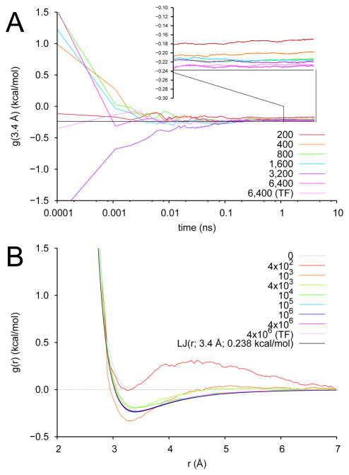
Results appear in Fig. 4. In Fig. 4A, we show the convergence of the effective potential for various values of k, measured as the value of the potential at its minimum. We observe convergence by about 1 ns of integration, with the degree of accuracy increasing as k increases. Even with the relatively aggressive k of 200 kcal/mol/Ų, the well-depth is only in error by about 25%, dropping to about 4% for k = 6,400 kcal/mol/Ų. Results from a single simulation at k = 6,400 kcal/mol/Ų run using TAMD-forces on z rather than analytical forces is also shown in this figure an indicates that there is no advantage in updating z using either analytical forces or TAMD forces in this case.

Fig. 4.

TAMD/OTFP parameterization of a 141-knot effective pair potential: the liquid Argon/Lennard-Jones test case. (A) Value of the pair potential at separation distance 3.4 Å vs time for various values of k. −0.238 kcal/mol is the well-depth of the input LJ potential. “TF” designates a simulation in which TAMD forces were used to update z; for all other simulations, analytical forces were used. (B) Effective pair potential g(r; λ(t)) at various times during the TAMD/OTFP simulation. g is initialized with values from the WCA potential (“0”) and we show here it converges to the LJ potential (black).

In Fig. 4B, we show the effective potentials themselves from various time-points in the k = 6,400 simulation. Clearly we are successfully reconstructing the “true” free energy for this system using this approach, as the converged linearly interpolated effective pair potential is essentially indistinguishable from a Lennard-Jones pair potential with ε = 0.238 kcal/mol and r_min = 3.4 Å. The slight positive discrepancy reflects the mollification of the true free energy due to the harmonic springs.

5.2. Example 4: Derivation of Effective Potentials for Single-Site Water

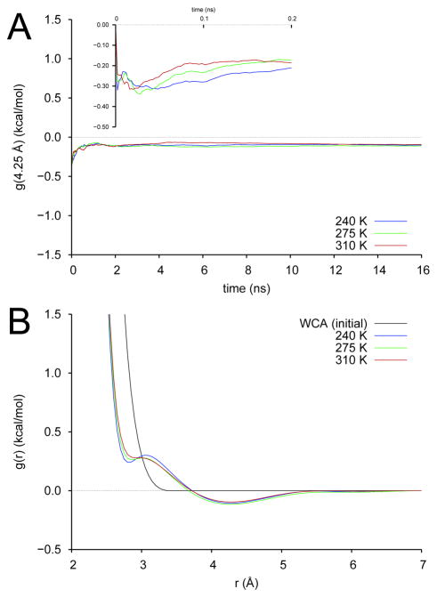
We now consider coarse-graining water onto single-site particles, which has be considered by in the past by many others. [13, 18, 21] Our all-atom system comprises 299 water molecules under the TIP3PE [23] model at a density of 1.00 g/cm³ in a cubic simulation volume. We take as z the cartesian coordinates of molecule centers of mass, and initialize the effective pair potential using the WCA potential with parameters ε = 0.5 kcal/mol and r_min = 2.6 Å, with a cutoff of 7 Å, with a total of 141 knots. As with the liquid argon case, the parameters λ are evolved only in the subspace where statistics are available, and the knot at 7 Å is held fixed at 0. We consider a single value of k of 1,600 kcal/mol-Ų and derive effective pair potentials at three temperatures: 240 K, 275 K, and 310 K. In each case, we used a fictitious thermal energy twice the physical thermal energy. All runs were carried out to 16 ns with a time-step of 2 fs and rigid bonds. Particle-mesh Ewald was used with a grid spacing of 1 Å. Here, in all simulations we update z using TAMD forces.

Fig. 5A illustrates convergence of the effective water potentials by showing the value of the potential at a separation distance of 4.25 Å, where all single-site water pair potentials show a broad, shallow minimum. Not surprisingly, these are slower to converge than the argon potentials due to the need for orientational sampling of the water molecules. The three potentials are plotted in Fig. 5B. We observe the characteristic shoulder at low separations and the well at 4.25 Å observed for water pair potentials derived by relative entropy minimization [18] and force-matching. [15] The trends with temperature are also in agreement with this previous work. [18] This clearly demonstrates that TAMD/OTFP is a viable means for deriving effective pair potentials for molecular coarse-graining. We defer to a later study an evaluation of these potentials in coarse-grained simulations.

Fig. 5.

TAMD/OTFP parameterization of a 141-knot effective pair potential: single-site coarse-graining of TIP3PE water. (A) Value of the pair potential at separation distance 4.25 Å vs time for three physical temperatures. (B) Effective pair potentials g(r; λ) for three physical temperatures.

6. Conclusions

We have proposed a new method for parameterizing free energies in collective variables from stochastic and dynamic simulations. The method, termed “Temperature Accelerated MD/On-The-Fly Parameterization”, or TAMD/OTFP for short, permits the determination of optimal parameter values in a free energy of a known functional form. We illustrated that TAMD/OTFP recapitulates parameters in a given potential energy when the fundamental variables in a dynamical system are taken also as collective variables, as shown in both a simple 1D example and an MD simulations of liquid argon. In particular, we demonstrated the utility of TAMD/OTFP in deriving effective pair potentials. We suggest therefore that TAMD/OTFP may be a useful method for deriving coarse-grained free energies in a wide variety of molecular and other dynamical simulation methods. It is worth mentioning, because of the simplicity of the CV’s we have chosen for this work, that AFED [12] might work as an alternative method for computing free energy gradients. However, because AFED requires relatively complicated transformations of equations of motion for CV’s that are nonlinear functions of atomic coordinates, it may be a less convenient choice than TAMD or d-AFED when moving to such more general CV’s.

Finally, we note that although it is permissible to cast the TAMD/OTFP system within the HMM framework (Eq. 7), we did not really explore this here because our free energies were relatively simple, and TAMD forces were equally efficacious in updating z as analytical forces in our examples. However, this feature could prove especially useful in situations where the CVs are a field, so that their equation of motion is a partial differential equation subject to CFL conditions of stability, which is a topic we are currently pursuing.

Highlights.

• Our method can determine parameters of a free energy in molecular simulations

• Free-energy gradients from temperature-accelerated MD are used on-the-fly

• We demonstrate our method in derived effective potentials for coarse-grained simulations

References

- 1.Sprik M, Ciccotti G. J Chem Phys. 1998;109:7737–7744. [Google Scholar]
- 2.Kumar S, Bouzidia D, Swendsen RH, Kollman PA, Rosenberg JM. J Comput Chem. 1992;13:1011–1021. [Google Scholar]
- 3.Jarzynski C. Phys Rev Lett. 1997;78:2690–2693. [Google Scholar]
- 4.Park S, Khalili-Araghi F, Tajkhorshid E, Schulten K. J Chem Phys. 2003;119:3559–3566. [Google Scholar]
- 5.Laio A, Parrinello M. Proc Natl Acad Sci USA. 2002;99:12562–12566. doi: 10.1073/pnas.202427399. [DOI] [PMC free article] [PubMed] [Google Scholar]
- 6.Maragliano L, Vanden-Eijnden E. J Chem Phys. 2008;128:184110. doi: 10.1063/1.2907241. [DOI] [PubMed] [Google Scholar]
- 7.Ren WEW, Vanden-Eijnden E. Phys Rev B. 2002;66:052301. [Google Scholar]
- 8.Maragliano L, Fischer A, Vanden-Eijnden E, Ciccotti G. J Chem Phys. 2006;125:024106. doi: 10.1063/1.2212942. [DOI] [PubMed] [Google Scholar]
- 9.Maragliano L, Vanden-Eijnden E. Chem Phys Lett. 2006;426:168–175. [Google Scholar]
- 10.Abrams C, Vanden-Eijnden E. Proc Natl Acad Sci USA. 2010;107:4961–4966. doi: 10.1073/pnas.0914540107. [DOI] [PMC free article] [PubMed] [Google Scholar]
- 11.Abrams J, Tuckerman ME. J Phys Chem B. 2008;112:15742–15757. doi: 10.1021/jp805039u. [DOI] [PubMed] [Google Scholar]
- 12.Rosso L, Minary P, Zhu ZW, Tuckerman ME. J Chem Phys. 2002;116:4389–4402. [Google Scholar]
- 13.Soper AK. Chem Phys. 1996;202:295–306. [Google Scholar]
- 14.Reith D, Pütz M, Müller-Plathe F. J Comput Chem. 2003;24:1624–1636. doi: 10.1002/jcc.10307. [DOI] [PubMed] [Google Scholar]
- 15.Izvekov S, Voth GA. J Chem Phys. 2005;123:134105. doi: 10.1063/1.2038787. [DOI] [PubMed] [Google Scholar]
- 16.Izvekov S, Voth GA. J Phys Chem B. 2005;109:2469–2473. doi: 10.1021/jp044629q. [DOI] [PubMed] [Google Scholar]
- 17.Noid WG, Chu JW, Ayton GS, Krishna V, Izvekov S, Voth GA, Das A, Andersen HC. J Chem Phys. 2008;128:244114. doi: 10.1063/1.2938860. [DOI] [PMC free article] [PubMed] [Google Scholar]
- 18.Chaimovich A, Shell MS. Phys Chem Chem Phys. 2009;11:1901–1915. doi: 10.1039/b818512c. [DOI] [PubMed] [Google Scholar]
- 19.WE, Engquist B. Comm Math Sci. 2003;1:87–132. [Google Scholar]
- 20.WE, Engquist B, Li X, Ren W, Vanden-Eijnden E. Comm Comput Phys. 2007;2(3):367–450. [Google Scholar]
- 21.Izvekov S, Voth GA. J Phys Chem B. 2005;109(7):2469–73. doi: 10.1021/jp044629q. [DOI] [PubMed] [Google Scholar]
- 22.Weeks JD, Chandler D, Andersen HC. J Chem Phys. 1971;54(12):5237–5247. [Google Scholar]
- 23.Price DJ, Brooks CL., III J Chem Phys. 2004;121(20):10096–103. doi: 10.1063/1.1808117. [DOI] [PubMed] [Google Scholar]