Decline in Genetic Influence on th Co-Occurrence of Alcohol, Marijuana, and Nicotine Dependence Symptoms from Age 14 to 29?

Abstract

Objective

Cross-sectional studies have demonstrated high rates of comorbidity among substance use disorders. However, few studies have examined the developmental course of incident comorbidity, and how it changes from adolescence to adulthood. Patterns of comorbidity among substance use disorders provides insight into the effect of shared versus specific etiological influences on measures of substance abuse and dependence.

Method

We evaluated the pattern of correlations among nicotine, alcohol, and marijuana abuse and dependence symptom counts as well as their underlying genetic and environmental influences in a community-representative twin sample (N=3762). Symptoms were assessed at ages 11, 14, 17, 20, 24, and 29. A single common factor was used to model the correlations among symptom counts at each age. Age-related changes in the influence of this general factor were examined by testing for differences in the mean factor loading across time.

Results

Mean levels of abuse/dependence symptoms increased throughout adolescence, peaked around age20, and declined from age 24 to 29. The influence of the general factor was highest at ages 14 and 17, but decreased from age 17 to 24. Genetic influences of the general factor declined considerably with age, along with an increase in non-shared environmental influences.

Conclusions

Adolescent substance abuse/dependence is largely a function of shared etiology. As individuals age, symptoms are increasingly influenced by substance-specific etiological factors. Heritability analyses showed that the generalized risk is primarily influenced by genetic factors in adolescence, but non-shared environmental influences increase in importance as substance dependence becomes more specialized in adulthood.

Epidemiological studies have documented high rates of comorbidity among alcohol, nicotine, and illicit drug dependence disorders (1–5). Comorbidity suggests that these nosologically distinct disorders are caused, in part, by common etiological processes (6-8). In substance use disorders, the etiology shared among disorders indexed by comorbidity has been referred to as “externalizing” or “disinhibitory psychopathology” (9).

While comorbidity among substance use disorders has been extensively studied cross-sectionally—typically for lifetime prevalence rates—few studies have examined how comorbidity changes over time, an important topic given the large changes in incidence over the lifespan. Specifically, substance use tends to emerge in middle adolescence, increases substantially throughout adolescence, peaks in the early 20’s, plateaus and then decreases in the late 20’s (10). Whether the rates of comorbidity among substance use disorders remain consistently high, however, is unknown. For example, rates of comorbidity might decline suggesting individuals begin to specialize in their substance use over time.

To investigate this, we used a large, longitudinal twin study to examine change in correlations among substance use disorder symptom counts over time. Assessments coincided with key developmental transitions in substance use including prior to initiation (age 11), initiation (age 14), regular use (age 17), heavy use and dependence (age 20 and 24), and the period when individuals decrease their use or exhibit patterns of persistent substance use problems (age 29). First, we examined patterns of mean-level change in nicotine, alcohol, and marijuana dependence symptoms. Second, we fit a single common factor model to account for the correlations among incident symptom counts of nicotine, alcohol, and marijuana at each age. This common factor model then allowed us to test for changes in the contribution of common and specific etiological influences on these disorder symptom counts across time. Third, we used standard twin models to estimate genetic and environmental influences on the common factor over time.

In addition to using the full sample, we also fit separate models to a subsample of early-onset users. We did so because estimates of correlations at earlier ages may be due to a minority of high-risk individuals who tend to exhibit dependence symptoms for multiple substances. Within this high-risk sample then correlations among dependence symptoms may remain high into adulthood. This could be obscured, however, in analyses of the full sample as substance use becomes more normative in adulthood. That is, if the correlations among substance use disorders are lower for the larger group of later-onset users, what is actually an artifact of early-versus later-onset use would appear to be an overall decline in the correlations among substance use disorders. We thus performed our analyses both for the full sample, and in a subsample of participants who had at least one symptom by their age-17 assessment, prior to the age at which any of these substances become legal in the United States.

Method

Sample

Participants (N=3762; 52% female) were drawn from the Minnesota Twin Family Study, a community -representative longitudinal study of Minnesota families (11). The younger twin cohort (N=2510; 51% female) was first assessed at age 11 during the years 1988–2005. The older cohort was first assessed at age 17 (N=1252; 54% female) during the years 1989–1996. Members of the 11-year old cohort were invited to participate in follow-up assessments at age 14 and 17, and all twins were invited to participate in follow -up assessments at age 20, 24, and 29. Cohorts were combined for all analyses. Participants received modest payments for their assessments. Written assent or consent was obtained from all participants, including the parents of minor children, and all study protocols were approved by the University of Minnesota IRB.

Additional analyses were conducted with a subsample of participants who had at least one symptom by their age-17 assessment for nicotine, alcohol, or marijuana dependence. This resulted in an “early-use” subsample of 580 males and 486 females.

Pooling across cohorts in the full sample, the actual ages of assessment were 11.8 (SD=0.4), 14.9 (0.6), 17.8 (0.7), 21.1 (0.8), 25.0 (0.9), and 29.5 (0.7) years. Participation rates ranged from 87.3% to 93.6% for the follow-up assessments. To examine attrition, we compared 17-year-olds who did versus did not complete the adult assessments at age 20, 24, and 29. For males, Cohen’s d for mean differences in age 17 dependence symptoms between those who did (N=1570) versus did not (N=238) complete the later assessments were .00, −.08, and .09 for nicotine, alcohol, and marijuana, respectively. For females, Cohen d’s for similar comparisons were −.19, −.01, and .13 (all p’s>.05).

Measures

Diagnostic symptom counts were obtained during in-person interviews with trained interviewers. In a consensus process, graduate students and staff with advanced training in clinical assessment reviewed cases to verify symptom presence.

At the age-11 and age-14 assessments, participants were assessed for DSM-III-R (12) nicotine dependence, alcohol dependence/abuse, and marijuana dependence/abuse using the Diagnostic Interview for Children and Adolescents (DICA-R; (13)). All later assessments used a modified version of the Substance Abuse Module (SAM; (14)) of the Composite International Diagnostic Interview (CIDI; (15)) to assess DSM-III-R symptoms of substance use disorders. Abuse and dependence symptoms were collapsed for alcohol and marijuana. Mother reports of their children’s symptoms were also obtained at ages 11, 14, and 17. The follow-up assessments at each age covered the interval elapsing since the last assessment. A “best -estimate” approach (16) was used whereby a symptom was considered present if reported by either the child or mother. Diagnostic inter-rater reliability of substance use disorders was greater than .91 (17). To rule out possible informant effects, all analyses were repeated using only the child as the informant. The pattern of results was identical.

Analysis of Change in Comorbidity

Bivariate correlations were computed using Spearman’s rho statistic, a rank-order statistic robust to departures from bivariate normality (18). Confirmatory factor analysis (19) was used to model the pattern of correlations among substance use disorders over time. For each assessment age, a single factor was fit to account for correlations among symptom counts of alcohol, nicotine, and marijuana dependence. Due to prohibitively low variance, symptoms at age 11 were not included in the model. This resulted in a model with five general factors, one for each age of assessment, and each representing the covariance among substance use disorders at each age. All factors were allowed to correlate, and all same-drug residuals were allowed to correlate across ages to account for the within-person correlated nature of the longitudinal data. Loadings were standardized. As such, the variance of the symptom count variables can be modeled as a function of the general and residual (substance specific) factors:

$$\text{Var}(\text{Symptom}\text{Count})={(\text{Factor}\text{Loading})}^2\times \text{Var}(\text{General}\text{Factor})+{(\text{Residual})}^2,$$

where “Var” denotes variance. Since the variance of the general factor was set to 1, the variance in a standardized symptom count accounted for by the general factor is simply the square of the factor loading. To obtain a single estimate of comorbidity for each age of assessment (i.e., a single estimate of the variance in the three symptom counts accounted for by the general factor), we calculated the mean squared factor loadings at each age. The mean squared loading provides a reasonable metric to test for changes in correlations, because it is directly proportional to the magnitude of correlations among the symptom count variables (i.e., higher correlations among the symptom counts results in greater mean variance in the symptom counts accounted for by the general factor). To test for significant differences, we constrained the mean squared loading to be the same across assessment waves, and conducted likelihood ratio tests to evaluate the change in model fit according to standard practice (20).

In addition, because the sample was composed of twins, we used standard twin modeling to decompose the general factor variances into three components: additive genetic (A), shared environment (C), and non-shared environment (E). All analyses were conducted in the same model rather than separate phenotypic and biometric models. Because we set the variance of the general factor to 1, the sum of the A, C, and E variance components of the general factors is also 1. To obtain the average variance in the symptom counts accounted for by genetic influences on the factor, one simply substitutes the term “Var (General Factor)” in the above equation with the corresponding genetic, shared environmental, or non-shared environmental component of the general factor variance. For example, if the age 17 mean squared loading was .4, then that would indicate that 40% of the variance in the symptom counts was due to the general factor. If the additive genetic component A of the age-17 factor was .7, then the genetic influence of the general factor onto the symptom counts would be .4×.7 =.28. That is, 28% of the symptom count variance would be due to the genetic influence of the factor.

Note that investigating the biometric decomposition of symptom count correlations is only applicable to the full sample, because the subsample analysis of individuals symptomatic by age 17 was, by definition, a within-individual analysis and disregards unaffected or later-affected (after age-17) co-twins. Resulting biometric decompositions would be difficult to interpret because included in the cross-twin correlations are only those pairs of twins both of whom were symptomatic by age 17.

Analyses were conducted using R version 2.10.1 (21). Open Mx version 1.0.6 (22) was used for the factor analysis. Missing data was handled using full information maximum likelihood. Model fit was evaluated using χ² tests and the difference in the Akaike Information Criterion (23) between the saturated and alternative models (positive values indicate the alternative provides better fit), separately for the four samples under study. We also report the root mean squared error of approximation, where values of .06 or less indicate a very good fit (24). The χ² test provides an exact test of model fit, but is sensitive to sample size and the magnitude of correlations among measures, and is always significant (p<.05) when statistical power is high (e.g., in large samples). It is often significant even when the model provides an accurate and useful representation of the data (25). As such, other fit indices have been developed and are primarily used to evaluate model fit. The root mean square error of approximation attempts to correct deficiencies of the χ² by adjusting for the degrees of freedom and sample size. Conventional RMSEA cutoffs are .08 for good fit and .05 for very good fit. The Akaike Information Criterion has strong theoretical properties in that the selected model is expected to fit best upon cross-validation (23).

Results

Longitudinal trends in symptom counts are somewhat different for males and females (Figure 1 and Table 1). For males, symptom counts significantly increase from age 11 to late adolescence, peak during the early 20’s, and decline thereafter. For females there is a more prolonged plateau during the late teens and early 20’s with a marked drop only by age 29. Mean symptom counts increased more rapidly for males than females, with males maintaining higher mean-level symptoms after age 14. Variances also increased during adolescence, and decreased during the late 20’s.

Figure 1.

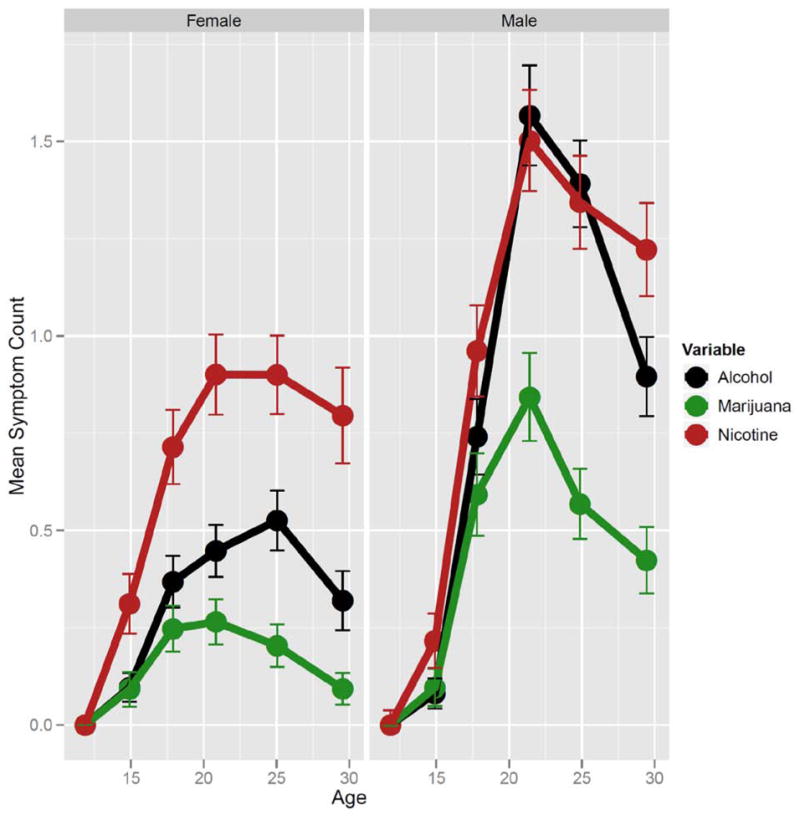
Mean Change in Symptom Count with Age. Females are displayed on the left and males on the right. Each substance is plotted in a different color. Means for Nicotine Dependence, Alcohol Dependence, and Marijuana Dependence are in red, black, and green, respectively. Error bars represent 95% confidence intervals.

Table 1.

Nicotine, Alcohol, and Marijuana Use and Misuse from Age 11 to 29.

Target Age of Assessment	Substance	N		% Ever Used Substance		Prevalence Of Dependence (%)		Prevalence of Subclinical Dependence (%with 1 or 2 Symptoms)		Mean Symptom Count		SD of Symptom Count		Sex Differences in Mean Symptom Counta	Sex Differences in Variance of Symptom Countb
		M	F	M	F	M	F	M	F	M	F	M	F	Effect Size	M/F Ratio
11	Nicotine	1233	1282	9	4	0.2	0.1	0.3	0.0	0.02	0.00	0.25	.08	N/A	N/A
	Alcohol	1233	1281	8	2	0.0	0.0	0.1	0.0	0.00	0.00	0.03	0.00	N/A	N/A
	Marijuana	1233	1282	1	0.4	0.0	0.0	0.0	0.0	0.00	0.00	0.03	0.00	N/A	N/A
14	Nicotine	1148	1191	35	27	4.5	4.6	3.5	2.8	0.22	0.31	0.99	1.15	−0.08	0.74***
	Alcohol	1132	1191	53	41	1.7	0.6	3.1	3.2	0.08	0.08	0.54	0.55	0.00	0.96
	Marijuana	1132	1191	13	10	1.7	1.4	2.4	1.5	0.09	0.08	0.67	0.62	0.02	1.17*
17	Nicotine	1129	1644	69	54	17.1	12.5	11.2	8.6	0.96	0.72	1.82	1.62	0.14**	1.26***
	Alcohol	1420	1644	79	77	11.1	4.9	23.6	13.3	0.74	0.37	1.55	1.19	0.27***	1.70***
	Marijuana	1423	1644	34	30	9.2	3.2	9.5	5.7	0.59	0.26	1.67	1.02	0.24***	2.68***
20	Nicotine	1393	1331	87	72	27.4	17.0	15.1	12.0	1.50	0.90	1.95	1.63	0.33***	1.43***
	Alcohol	1101	1331	96	96	24.6	6.2	30.0	15.6	1.56	0.44	1.93	1.12	0.73***	2.97***
	Marijuana	1111	1330	55	45	11.8	3.8	13.4	6.8	0.84	0.27	1.69	0.97	0.42***	3.04***
24	Nicotine	1009	1213	90	77	26.4	17.3	14.1	12.5	1.34	0.90	1.83	1.60	0.26***	1.31***
	Alcohol	1148	1213	98	98	23.0	6.9	32.0	17.8	1.39	0.52	1.76	1.23	0.58***	2.05***
	Marijuana	1143	1211	60	50	7.4	3.1	13.2	5.4	0.56	0.20	1.39	0.85	0.31***	2.67***
29	Nicotine	957	636	90	79	23.1	15.7	16.2	10.9	1.22	0.79	1.77	1.55	0.26***	1.30**
	Alcohol	957	636	98	97	12.9	4.5	27.4	11.2	0.89	0.31	1.52	0.95	0.44***	2.56***
	Marijuana	955	635	60	46	5.5	0.6	8.0	3.7	0.42	0.09	1.25	0.52	0.32***	5.78***

M refers to males; F to females.

^aSex differences in mean symptom count were evaluated with a likelihood ratio test correcting for within family correlations. Tabled values are Cohen’s d.

^bThe equality of variance across sex is given as a simple ratio of male variance to female variance, but again tested by correcting for within-family correlations.

^*p < .05;

^**p < .01,

^***p <.001.

Prevalence and symptom counts were measured in a since-last-assessment format.

The prevalence rates for each disorder and the proportion of individuals who had ever used each substance for each age are reported in Table 1. The mean participant age of initiation was 14.4 (SD=3.4) for nicotine, 15.5 (SD=2.6) for alcohol use without parental permission, and 16.5 (SD=2.5) years for marijuana. The mean age of symptom onset was 17.5 (SD = 2.7) for nicotine, 18.2 (SD=4.4) for alcohol, and 17.2 (SD = 2.3) for marijuana.

Cross-drug correlations decrease with age, as can be seen in the full bivariate correlation matrix reported in Figure 2. For example, for males, the correlation between nicotine and alcohol declines from .61 at age 14 to .26 at age 29.

Figure 2.

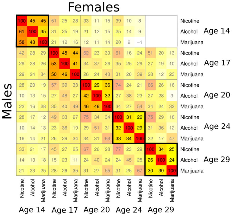
Within and Across Age Correlations between Substance Use Symptom Count Measures. Males are reported in the lower triangle and females in the upper triangle. Correlations (without decimals) are displayed within each colored box. To aid visualization, the matrix is a heat map, with hotter colors signifying higher correlations. The matrix is organized into blocks by age. Note the trend in the bolded diagonal blocks; the colors generally become cooler as one moves from the upper left to lower right, indicating a steady decrease in correlations among the substances over time. The off-diagonals have purposefully been partially obscured to focus the reader’s attention on the block diagonal without omitting relevant information about the cross-age correlations. Females in the younger cohort had just begun their age-29 assessment, and thus the age-14/age-29 block is empty.

Factor models were fit to provide a formal test of changes in the cross-drug correlations. Model fit in the full male sample was very good (χ²=216.66, df=170, p=.009; ΔAkaike Information Criterion = 123.33; Root Mean Square Error of Approximation = .02). Model fit in the full female sample was also good (χ²=432.32, df=170, p<.001; ΔAkaike Information Criterion = −92.32; Root Mean Square Error of Approximation = .05). Model fit was good in both the male (χ²=137.45, df=170, p=.97; ΔAkaike Information Criterion = 202.55; Root Mean Square Error of Approximation < .01) and female (χ²=133.42, df=106, p=.04; ΔAkaike Information Criterion = 78.6; Root Mean Square Error of Approximation = .04) early-use subsamples.

For each model, the size of the standardized factor loadings generally decreased with age, declining from .6–.8 at age 14 to .3–.6 at age 29, as reported in Table 2. The table also shows (as do the grey lines in Figure 3) that the mean squared loading, which served as our metric of change, declined with age. Recall that the mean squared loading provides the average variance in the symptoms accounted for by the general factor. To illustrate how these estimates are calculated, we enter the loadings from Table 2 into for the full female sample. The mean squared loading was (.65²+.71²+.79²)/3=.52 at age 14, and (.69²+.53²+.33²)/3=.29 at age 29. To test if the age 14 to 29 decline was statistically significant, we constrained the mean squared loadings to be same at each age and examined decrement in model fit. The likelihood ratio test indicated a significant decline in the mean squared loading from age 14 to age 29 for all samples: full male sample (χ²=158.4, df=4, p=3.2×10⁻³³), full female sample (χ²=146.97, df=4, p=9.1×10⁻³¹), male subsample of early users (χ²=54.66, df=4, p=3.8×10⁻¹¹), and from age 14 to 24 for the female subsample of early users (χ²=21.36, df=3, p=8.9×10⁻⁵). We tested for sex differences by comparing the fit of an unconstrained model to that of a model that constrained the mean squared loading to be equal across males and females. Relative to males, females showed an earlier decline in comorbidity at age 20 (χ²=24.18, df=1, p=8.8×10⁻⁷), but at no other ages.

Table 2.

Standardized Factor loadings and Factor Variance Components for Each Age of Assessment in the Four Samples.

	Factor Loadings								Factor Variance ACE Components
	Nicotine		Alcohol		Marijuana		Mean Squared Loading		A		C		E
	Est.	95% c.i.	Est.	95% c.i.	Est.	95% c.i.	Est.	95% c.i.	Est.	95% c.i.	Est.	95% c.i.	Est.	95% c.i.
Full Female Sample (N=1907)
Age 14	.65	(.59, .70)	.71	(.66, .83)	.79	(.74, .84)	.52	(.48, .56)	-	-	-	-	-	-
Age 17	.60	(.55, .64)	.78	(.74, .81)	.73	(.68, .83)	.51	(.47, .54)	.72	(.56, .88)	.14	(.27, .29)	.14	(.10, .19)
Age 20	.51	(.45, .58)	.57	(.50, .64)	.60	(.54, .65)	.32	(.28, .36)	.42	(.14, .74)	.21	(0, .47)	.37	(.25, .49)
Age 24	.60	(.53, .60)	.54	(.46, .61)	.39	(.31, .45)	.27	(.24, .31)	.61	(.31, .61)	.09	(0, .34)	.30	(.19, .42)
Age 29	.69	(.60, .79)	.53	(.43, .62)	.33	(.25, .41)	.29	(.24, .33)	.36	(.09, .61)	.12	(0, .39)	.53	(.36, .68)
Full Male Sample (N=1775)
Age 14	.74	(.69, .77)	.76	(.71, .80)	.77	(.73, .81)	.57	(.54, .61)	.35	(.16, .57)	.46	(.26, .63)	.19	(.14, .24)
Age 17	.70	(.65, .74)	.79	(.75, .82)	.72	(.67, .76)	.54	(.51, .57)	.69	(.50, .88)	.18	(.03, .36)	.14	(.10, .18)
Age 20	.65	(.60, .70)	.67	(.62, .72)	.70	(.64, .75)	.45	(.42, .49)	.58	(.37, .73)	.13	(.01, .32)	.29	(.22, .38)
Age 24	.55	(.48, .61)	.56	(.50, .62)	.56	(.49, .62)	.31	(.27, .35)	.54	(.30, .73)	.16	(.01, .39)	.30	(.19, .42)
Age 29	.47	(.41, .54)	.62	(.55, .69)	.59	(.52, .65)	.32	(.28, .36)	.47	(.47, .63)	.05	(0, .26)	.48	(.34, .61)
Females with at least 1 Symptom by Age 17 (N=486)
Age 14	.49	(.35, .61)	.64	(.52, .74)	.82	(.69, .93)	.44	(.36, .51)	-	-	-	-	-	-
Age 17	.32	(.21, .42)	.58	(.46, .69)	.77	(.65, .89)	.34	(.29, .40)	-	-	-	-	-	-
Age 20	.23	(.12, .35)	.52	(.32, .73)	.68	(.49, .91)	.26	(.20, .34)	-	-	-	-	-	-
Age 24	.31	(.17, .44)	.63	(.48, .76)	.43	(.28, .59)	.22	(.16, .29)	-	-	-	-	-	-
Age 29	-	-	-	-	-	-	-	-	-	-	-	-	-	-
Males with at least 1 Symptom by Age 17 (N=580)
Age 14	.69	(.61, .76)	.73	(.64, .80)	.76	(.68, .83)	.53	(.47, .59)	-	-	-	-	-	-
Age 17	.47	(.37, .56)	.62	(.52, .72)	.65	(.55, .76)	.35	(.29, .41)	-	-	-	-	-	-
Age 20	.49	(.39, .59)	.57	(.46, .67)	.68	(.55, .81)	.35	(.28, .41)	-	-	-	-	-	-
Age 24	.40	(.28, .52)	.49	(.36, .62)	.48	(.34, .62)	.21	(.15, .28)	-	-	-	-	-	-
Age 29	.43	(.21, .44)	.61	(.48, .75)	.64	(.50, .79)	.30	(.24, .36)	-	-	-	-	-	-

“Est.” is the maximum likelihood estimate and “95% c.i.” the 95% confidence interval around that estimate. The “Average Squared Loading” is simply the average of the squared loadings listed for that age. Age-29 data is not available for the female subsample because the assessment is ongoing. A refers to the additive genetic variance component of the factors, C to the shared environmental component, and E to the non-shared environmental component. A, C, and E estimates for the 14-year-old samples were poorly estimated due to lack of cross-twin co-variance in the symptom counts at that age (see Results), and are not provided for the females. A, C, and E estimates are not provided for the subsamples of early onset users because these samples are, by definition, within-individual and exclude co-twins who did not exhibit symptoms at the age-17 assessment. Resulting ACE estimates are therefore difficult to interpret.

Figure 3.

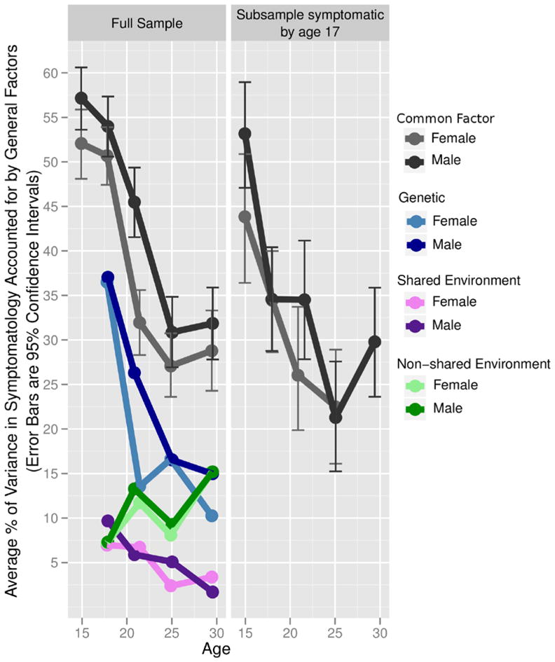
Percent of Symptom Count Variance Accounted for by the General Factor at Each Age. The grey lines in the figure show the decline in correlations over time as expressed by decline in the average percentage of variance accounted for by a general factor at each time point (i.e., the “Mean Squared Loading” column from Table 3). The full sample is shown on the left while the subsample of individuals who had atleast one nicotine, alcohol, or marijuana symptom by their age-17 assessment is shown on the right. The decline for both sexes in both samples was statistically significant (see Results). Sample sizes are given in the text as well as in Table 2. In the full male and female samples the blue, green, and purple lines represent the proportions of the general factor phenotypic variance (grey lines) that are due to genetic (blue), shared environmental (purple), and non-shared environmental (green) variance. Male values are always represented by the darker hue. These estimates can be computed directly from values provided in Table 3 by multiplying the mean squared loading by the corresponding ACE value (e.g., by the A value to obtain the additive genetic variance which is plotted in blue). The majority of phenotypic decline in the full sample is due to a statistically significant decline in heritability, as well as a non-statistically significant decline in shared environmental variance. In contrast, non-shared environmental variance significantly increases with age. Note that age-14 estimates are not given because girls at this age had few symptoms (see Results). Genetic and environmental components are not given for the subsample as it was composed of selected individuals, and not selected twin pairs (see Methods).

Table 2 provides the A, C, and E components of each age’s general factor, for each sample. While these estimates are useful, they must be multiplied by their respective factor loadings to determine the genetic and environmental impact on the individual symptom counts. To do this, we replaced the Var (Factor) term in Equation 1 with the A, C, and E variance components. The resulting values are displayed for each age in the left panel of Figure 3. Note that the scaling is such that adding the A (blue), C (purple), and E (green) components reproduce the mean squared loading (grey; also listed in Table 2). For example, at age 29 for males the phenotypic variance accounted for by the general factor was 32%, which was composed of 15% (.32×.47×100%) additive genetic variance, 15% (.32×.48×100%) non-shared environment, and 2% (.32×.05×100%) shared environment (15%+15%+2%=32%). Unfortunately, symptoms were expressed relatively infrequently by both members of a female twin pair at age 14, rendering the age-14 additive genetic, shared environmental, and non-shared environmental components poorly estimated and hence excluded from Figure 3 along with the male estimates for consistency.

We tested for change in heritability, shared environment, and non-shared environment estimates in Figure 3 by fixing relevant parameters to be equal at ages 17, 20, 24, and 29, testing for decrements in model fit. For example, to test for a change in heritability, we fixed the A component of each general factor to be equal, and tested the fit of this model against the original model where all A components are freely estimated. The decline in heritability noticed in Figure 3 was significant for males (χ²=23.86, df=3, p=2.7×10⁻⁵) and females (χ²=26.6, df=3, p=7.0×10⁻⁶). It appears thus that the vast majority of the phenotypic decline in Figure 3 is due to a decline in genetic variance. The increase in non-shared environment was also significant for males (χ²=15.73, df=3, p=.001) and females (χ²=11.48, df=3, p=.009). Changes in shared environment were not significant in either sex.

Discussion

We examined changes in the correlations among symptoms of nicotine, alcohol, and marijuana abuse and dependence from age 11 to 29. As seen in Figure 3, males and females show significant declines in these correlations from adolescence to adulthood. This was also true for an early-onset subsample of individuals with at least one symptom of nicotine, alcohol, or marijuana dependence by age 17. Correlation among disorders or their symptoms is evidence that those disorders share etiology. The results suggest that the shared etiology contributing to nicotine, alcohol, and marijuana dependence symptoms diminish over time. That is, younger individuals tended to use these three substances indiscriminately, whereas older individuals began to show a preference for one substance over others. Despite declines in the correlations, the rates of use (Figure 1) continued to climb throughout late adolescence and early adulthood. Finally, after age 17 the correlations among symptoms became less attributable to pleiotropic genetic effects and increasingly a result of non-shared environmental influences (Figure 3), indicating that the types of etiological processes contributing to the variation in use of multiple drugs is gradually changing during the transition to adulthood.

Several processes might contribute to the transition from general to specific influences. For one, adolescents are more impulsive and risk-taking than adults (26). Personality traits such as disinhibition and sensation-seeking are not predispositions to use any particular substance, but rather to use whatever substances might be available (9, 27). Additionally, neurodevelopmental changes relevant to behavioral disinhibition continue throughout adolescence. For example, by adolescence, the nucleus accumbens—important in reward sensitivity—is well-developed, but poorly regulated by a still maturing prefrontal cortex (28–29), resulting in deficits of top-down control over the reward system that slowly improves into early adulthood. This developmental window is the same time period that we observed decreases in the comorbidity among different substance use disorders, suggesting that disinhibitory mechanisms with known neurological substrates may be in play. Further supporting this hypothesis, the earlier decline in comorbidity for females relative to males from age 17 to 20 (Figure 3) is consistent with the earlier pubertal (30), cortical (31), and personality (32) maturation in females compared to males.

Our results are consistent with individual differences in drug reinforcement. That is, initial drug use that begins in adolescence is characterized by relatively indiscriminant experimentation. Due to individual differences in the reinforcing effects of different drugs, however, people may tend eventually to restrict their use to those drugs that provide the greatest reinforcement. There are myriad etiological mechanisms relevant to individual differences in drug reinforcement, including drug metabolism effects, drug availability, social rewards and punishments, and differences in drug-specific neurological sensitivity that may further be moderated by drug and alcohol neurotoxic mechanisms (27, 33). Future research might consider these covariates in characterizing the transition to substance specialization.

While consistent with the theory that disinhibition accounts for comorbidity among substance use disorders, the results are not entirely inconsistent with the gateway hypothesis (34). The gateway hypothesis holds that using one drug leads to using other drugs, perhaps due to the experienced high and an increased desire to obtain bigger and better highs. If correct, the theory would predict the opposite pattern of comorbidity we observed; that is, correlations should be low at younger ages and increase over time. At younger ages, most people would not yet have used their first or second gateway drug, and would not have had time to explore other drugs. Over time, the correlations among drugs should increase as the initial drug use would cause them to use other drugs. In fact, we found that as drug dependence symptoms increased (Figure 1), the magnitude of the associations among different drugs declined (Figure 3); opposite the pattern predicted by the gateway theory. This conclusion is consistent with a growing body of literature inconsistent with parts of the gateway theory (1, 9, 35–37). That said, the increase in non-shared environmental effects observed in Figure 3 could contain etiology analogous to a gateway process, in that there are environments experienced by an individual that contribute to dependence to multiple drugs in that person, but not that person’s co-twin. While the range of possible environments is vast and the effect is small, it could very well include drug use (e.g., impaired cognition caused by neurotoxicity) and/or other risk factors for non-specific drug use such as occupational, social, and legal problems.

Limitations

While a strength, the use of a community-representative sample may not apply to clinical populations. The fact that results were consistent for the subsample of individuals who were symptomatic at age 17suggests this is not a major concern. We used symptom counts because symptoms are relevant to the DSM clinical literature and provide measurement consistency from age 11 to 29. In supplementary analyses we evaluated other measures of quantity and frequency of nicotine, alcohol, and marijuana use (not shown). These measures had higher means and variances at younger ages, and resulted in the same trends as presented here for symptoms.

In the United States adolescent development is confounded with substance-use-relevant environmental changes. Adolescents gradually experience increased autonomy and financial freedom from caregivers. The purchase of tobacco and alcohol becomes legal at age 18 and 21, respectively, while marijuana use is always illegal. Undoubtedly, these environmental influences impacted symptom means and correlations. However, one cannot disentangle these influences from other behavioral and neurological changes, at least within a single culture. Cross-cultural and cross-generational studies, for example comparisons between societies that differ in drug laws, are required to unravel maturational and environmental changes during development.

References

- 1.Kendler KS, Jacobson KC, Prescott CA, Neale MC. Specificity of genetic and environmental risk factors for use and abuse/dependence of cannabis, cocaine, hallucinogens, sedatives, stimulants, and opiates in male twins. Am J Psychiat. 2003 Apr;160(4):687–95. doi: 10.1176/appi.ajp.160.4.687. [DOI] [PubMed] [Google Scholar]
- 2.Kendler KS, Prescott CA, Myers J, Neale MC. The structure of genetic and environmental risk factors for common psychiatric and substance use disorders in men and women. Arch Gen Psychiat. 2003 Sep;60(9):929–37. doi: 10.1001/archpsyc.60.9.929. [DOI] [PubMed] [Google Scholar]
- 3.Kessler RC, Chiu WT, Demler O, Merikangas KR, Walters EE. Prevalence, severity, and comorbidity of 12-month DSM-IV disorders in the national comorbidity survey replication. (vol 62, pg 617, 2005) Arch Gen Psychiat. 2005 Jul;62(7):709. doi: 10.1001/archpsyc.62.6.617. [DOI] [PMC free article] [PubMed] [Google Scholar]
- 4.Moffitt TE, Caspi A, Taylor A, Kokaua J, Milne BJ, Polanczyk G, et al. How common are common mental disorders? Evidence that lifetime prevalence rates are doubled by prospective versus retrospective ascertainment. Psychological Medicine. 2010 Jun;40(6):899–909. doi: 10.1017/S0033291709991036. [DOI] [PMC free article] [PubMed] [Google Scholar]
- 5.Krueger RF, Hicks BM, Patrick CJ, Carlson SR, Iacono WG, McGue M. Etiologic connections among substance dependence, antisocial behavior, and personality: Modeling the externalizing spectrum. J Abnorm Psychol. 2002 Aug;111(3):411–24. [PubMed] [Google Scholar]
- 6.Krueger RF, Markon KE. Reinterpreting comorbidity: A model-based approach to understanding and classifying psychopathology. Annu Rev Clin Psycho. 2006;2:111–33. doi: 10.1146/annurev.clinpsy.2.022305.095213. [DOI] [PMC free article] [PubMed] [Google Scholar]
- 7.Meehl PE. Comorbidity and taxometrics. Clin Psychol-Sci Pr. 2001 Win;8(4):507–19. [Google Scholar]
- 8.Meehl PE. Factors and Taxa, Traits and Types, Differences of Degree and Differences in Kind. J Pers. 1992 Mar;60(1):117–74. [Google Scholar]
- 9.Iacono WG, Malone SM, McGue M. Behavioral disinhibition and the development of early-onset addiction: Common and specific influences. Annu Rev Clin Psycho. 2008;4:325–48. doi: 10.1146/annurev.clinpsy.4.022007.141157. [DOI] [PubMed] [Google Scholar]
- 10.Young SE, Corley RP, Stallings MC, Rhee SH, Crowley TJ, Hewitt JK. Substance use, abuse and dependence in adolescence: prevalence, symptom profiles and correlates. Drug Alcohol Depen. 2002 Dec 1;68(3):309–22. doi: 10.1016/s0376-8716(02)00225-9. [DOI] [PubMed] [Google Scholar]
- 11.Iacono WG, McGue M. Minnesota Twin Family Study. Twin Res. 2002 Oct;5(5):482–7. doi: 10.1375/136905202320906327. [DOI] [PubMed] [Google Scholar]
- 12.American Psychiatric Association. Diagnostic and statistical manual of mental disorders. 3. Washington, D.C: Author; 1987. rev. [Google Scholar]
- 13.Welner Z, Reich W, Herjanic B, Jung KG, Amado H. Reliability, validity, and parent-child agreement studies of the Diagnostic Interview for Children and Adolescents (DICA) J Am Acad Child Adolesc Psychiatry. 1987 Sep;26(5):649–53. doi: 10.1097/00004583-198709000-00007. [DOI] [PubMed] [Google Scholar]
- 14.Robins LN, Babor TF, Cottler LB. Composite International Diagnostic Interview: Expanded Substance Abuse Module. St. Louis: Authors; 1987. [Google Scholar]
- 15.Robins LN, Wing J, Wittchen HU, Helzer JE, Babor TF, Burke J, et al. The Composite International Diagnostic Interview. An epidemiologic Instrument suitable for use in conjunction with different diagnostic systems and in different cultures. Arch Gen Psychiat. 1988;45(12):1069–77. doi: 10.1001/archpsyc.1988.01800360017003. [DOI] [PubMed] [Google Scholar]
- 16.Leckman JF, Scholomskas D, Thompson WD, Belanger A, Weisman MM. Best estimate of lifetime psychiatric diagnosis: A methodlogical study. Arch Gen Psychiat. 1982;39:879–83. doi: 10.1001/archpsyc.1982.04290080001001. [DOI] [PubMed] [Google Scholar]
- 17.Iacono WG, Carlson SR, Taylor J, Elkins IJ, McGue M. Behavioral disinhibition and the development of substance use disorders: Findings from the Minnesota Twin Family Study. Dev Psychopathol. 1999;11:869–900. doi: 10.1017/s0954579499002369. [DOI] [PubMed] [Google Scholar]
- 18.Caruso JC, Cliff N. Empirical size, coverage, and power of confidence intervals for Spearman’s rho. Educ Psychol Meas. 1997 Aug;57(4):637–54. [Google Scholar]
- 19.Brown T. Confirmatory Factor Analysis for Applied Research. New York: The Guilford Press; 2006. [Google Scholar]
- 20.Miller MB, Neale MC. Using Nonlinear Constraints in Mx to Automate Estimation of Confidence-Intervals for Parameters in Genetic Models. Behav Genet. 1995 May;25(3):279–80. [Google Scholar]
- 21.R Development Core Team. R: A language and environment for statistical computing. Vienna: R Foundation for Statistical Computing; 2011. [Google Scholar]
- 22.Boker S, Neale M, Maes H, Wilde M, Spiegel M, Brick T, et al. OpenMx: An Open Source Extended Structural Equation Modeling Framework. Psychometrika. 2011 Apr;76(2):306–17. doi: 10.1007/s11336-010-9200-6. [DOI] [PMC free article] [PubMed] [Google Scholar]
- 23.Vrieze SI. Model selection and psychological theory: A discussion of the differences between the Akaike Information Criterion (AIC) and the Bayesian Information Criterion (BIC) Psychol Methods. doi: 10.1037/a0027127. in press. [DOI] [PMC free article] [PubMed] [Google Scholar]
- 24.Hu LT, Bentler PM. Cutoff Criteria for Fit Indexes in Covariance Structure Analysis: Conventional Criteria Versus New Alternatives. Struct Equ Modeling. 1999;6(1):1–55. [Google Scholar]
- 25.Bentler PM. Comparative Fit Indexes in Structural Models. Psychol Bull. 1990 Mar;107(2):238–46. doi: 10.1037/0033-2909.107.2.238. [DOI] [PubMed] [Google Scholar]
- 26.Steinberg L, Cauffman E, Woolard J, Graham S, Banich M. Are Adolescents Less Mature Than Adults? Minors’ Access to Abortion, the Juvenile Death Penalty, and the Alleged APA “Flip-Flop”. Am Psychol. 2009 Oct;64(7):583–94. doi: 10.1037/a0014763. [DOI] [PubMed] [Google Scholar]
- 27.Bechara A. Decision making, impulse control and loss of willpower to resist drugs: a neurocognitive perspective. Nat Neurosci. 2005 Nov;8(11):1458–63. doi: 10.1038/nn1584. [DOI] [PubMed] [Google Scholar]
- 28.Casey BJ, Getz S, Galvan A. The adolescent brain. Dev Rev. 2008 Mar;28(1):62–77. doi: 10.1016/j.dr.2007.08.003. [DOI] [PMC free article] [PubMed] [Google Scholar]
- 29.Casey BJ, Tottenham N, Liston C, Durston S. Imaging the developing brain: what have we learned about cognitive development? Trends Cogn Sci. 2005 Mar;9(3):104–10. doi: 10.1016/j.tics.2005.01.011. [DOI] [PubMed] [Google Scholar]
- 30.Tanner JM, Whitehouse RH, Takaishi M. Standards from Birth to Maturity for Height, Weight, Height Velocity, and Weight Velocity: British Children, 1965. Part II. Archives of Disease in Childhood. 1966;41:613–35. doi: 10.1136/adc.41.220.613. [DOI] [PMC free article] [PubMed] [Google Scholar]
- 31.Lenroot RK, Gogtay N, Greenstein DK, Wells EM, Wallace GL, Clasen LS, et al. Sexual dimorphism of brain developmental trajectories during childhood and adolescence. Neuroimage. 2007 Jul 15;36(4):1065–73. doi: 10.1016/j.neuroimage.2007.03.053. [DOI] [PMC free article] [PubMed] [Google Scholar]
- 32.Klimstra TA, Hale WW, Raaijmakers AW, Branje SJT, Meeus WHJ. Maturation of Personality in Adolescence. J Pers Soc Psychol. 2009 Apr;96(4):898–912. doi: 10.1037/a0014746. [DOI] [PubMed] [Google Scholar]
- 33.Goldstein RZ, Volkow ND. Drug addiction and its underlying neurobiological basis: Neuroimaging evidence for the involvement of the frontal cortex. Am J Psychiat. 2002 Oct;159(10):1642–52. doi: 10.1176/appi.ajp.159.10.1642. [DOI] [PMC free article] [PubMed] [Google Scholar]
- 34.Kandel DB, Jessor R. The gateway hypothesis revisited. In: Kandel DB, editor. Stages and Pathways of Drug Involvement. New York: Cambridge University Press; 2002. [Google Scholar]
- 35.Tarter RE, Vanyukov M, Kirisci L, Reynolds M, Clark DB. Predictors of marijuana use in adolescents before and after licit drug use: Examination of the gateway hypothesis. Am J Psychiat. 2006 Dec;163(12):2134–40. doi: 10.1176/ajp.2006.163.12.2134. [DOI] [PubMed] [Google Scholar]
- 36.Vanyukov MM, Tarter RE, Kirisci L, Kirillova GP, Maher BS, Clark DB. Liability to substance use disorders: 1. Common mechanisms and manifestations. Neurosci Biobehav Rev. 2003 Oct;27(6):507–15. doi: 10.1016/j.neubiorev.2003.08.002. [DOI] [PubMed] [Google Scholar]
- 37.Irons DE, McGue M, Iacono WG, Oetting WS. Mendelian randomization: A novel test of the gateway hypothesis and models of gene-environment interplay. Dev Psychopathol. 2007 Fal;19(4):1181–95. doi: 10.1017/S0954579407000612. [DOI] [PubMed] [Google Scholar]