Abstract
Bayesian network model is widely used for reverse engineering of biological network structures. An advantage of this model is its capability to integrate prior knowledge into the model learning process, which can lead to improving the quality of the network reconstruction outcome. Some previous works have explored this area with focus on using prior knowledge of the direct molecular links, except for a few recent ones proposing to examine the effects of molecular orderings. In this study, we propose a Bayesian network model that can integrate both direct links and orderings into the model. Random weights are assigned to these two types of prior knowledge to alleviate bias toward certain types of information. We evaluate our model performance using both synthetic data and biological data for the RAF signaling network, and illustrate the significant improvement on network structure reconstruction of the proposing models over the existing methods. We also examine the correlation between the improvement and the abundance of ordering prior knowledge. To address the issue of generating prior knowledge, we propose an approach to automatically extract potential molecular orderings from knowledge resources such as Kyoto Encyclopedia of Genes and Genomes (KEGG) database and Gene Ontology (GO) annotation.
Key words: computational molecular biology, functional genomics
1. Introduction
Biological networks carry out their functions through well-organized molecular interactions. One way of studying their structures at a systematic scale is using Bayesian network models to find the network structure with maximum posterior probability, given expression data and prior knowledge (Friedman et al., 1998; Murphy and Mian, 1999; Friedman et al., 2000; Gifford and Jaakkola, 2001). A Bayesian network model describes the joint distribution of random variables, which are biological molecules in this case, through their dependence and conditional independence. It can facilitate the computation of posterior probability P(Gh|D, ξ), where Gh is a hypothesis network structure, D is the expression data, and ξ is the prior knowledge. From Bayes' law, we have
 |
where P(Gh|ξ) represents the prior probability of the hypothesis network and P(D|Gh, ξ) represents the marginal likelihood of data. Employing the Bayesian network model's definition and certain assumptions, the marginal likelihood can be calculated with a closed form formula (Heckerman and Chickering, 1995). The prior probability can also be decomposed into product of local conditional probabilities of all the variables as shown below:
 |
In the above equation, Xi is the ith node in the network Gh, Pa(Xi) is the set of parent nodes of Xi, and n is the total number of nodes in Gh. This decomposition greatly improves the efficiency of the prior probability computation (Cooper and Herskovits, 1992; Heckerman and Chickering, 1995; Segal et al., 2005).
Since the number of possible network structures is super-exponential to the number of nodes in a network, it is computationally infeasible for a Bayesian network model to enumerate all the possible network structures and find the global optimum. Traditionally, heuristic approaches such as hill climbing have been used to find the local maximum (Imoto et al., 2002; Ko et al., 2009). An alternative approach is to apply the Monte Carlo Markov Chain (MCMC) methods to find the posterior probability distribution of network structures directly (Geier et al., 2007; Grzegorczyk et al., 2008; Kaderali et al., 2009).
An appealing feature of Bayesian network models is their capability to integrate prior knowledge into reconstruction of biological networks. Some previous studies have examined the effects of including direct molecular interactions into prior probability P(Gh|ξ) (Imoto et al., 2003; Tamada et al., 2003; Nariai et al., 2004; Imoto et al., 2006; Husmeier and Werhli, 2007; Werhli and Husmeier, 2007; Perrier et al., 2008). Our own previous work also has tackled the approach of including molecular orderings, in addition to the direct interactions, into explicitly computing the prior probability (Pei et al., 2008). Basically, we assign fixed weights to both the direct links and the orderings prior knowledge and show their positive impact on Bayesian network model learning by using synthetic data.
In the present study, we extend our previous work (Pei et al., 2008) by proposing three improvements. First, we introduce random weights to both direct links and ordering relations in computing the posterior probabilities. This eliminates the artifacts stemming from the fixed weights on model performance and allows the model to adapt to the knowledge and data automatically. Second, we automatically derive prior knowledge from public databases such as GO and KEGG. And finally, we evaluate the performance of our model with real biological data, which is for the human RAF signal transduction network published by Sachs et al. (2005).
2. Methods
2.1. Integration of prior knowledge
The prior knowledge for direct links is defined by an n × n matrix L, where n is the number of variables in the network and each entry Lij represents prior confidence about variable i affecting variable j directly, ranging from 0 to 1. In addition, we also use the term “ordering” in the present study to represent knowledge of one molecule i affecting another target molecule j in a biological network without a direct link. We denote i as an ancestor of j and summarize the ordering prior knowledge with an n × n matrix K, where each entry Kij ranging from 0 to 1 represents prior confidence about whether variable i is an ancestor of variable j. We thus define the prior probability of a hypothesis network structure Gh as
 |
(1) |
where Z is a partition function, and EL(Gh) and EK(Gh) represent “energies” of Gh, which are derived, respectively, from matrices L and K as follows:
 |
(2) |
 |
(3) |
In the above equations, Bij and  indicate whether there is a direct link and an ordering relation from i to j in Gh, respectively, and ωl and ωk are weights for their respective two forms of energies. It can be seen that when a network structure becomes more consistent with the prior knowledge, it will have lower energy and higher prior probabilities, and hence the specific network structure is more likely to be obtained during the model learning procedure.
2.2. Partition function with random weights
The weights ωl and ωk in Equations (2) and (3) can be either constants or random variables. Constant weights simplify the computation but suffer from introducing a bias into the analysis outcome as we have already reported elsewhere (Pei et al., 2008). Hence we treat weights as random variables here and discuss how the partition function can be computed.
The partition function Z in Equation (1) is defined as
 |
(4) |
where  is the network structure space. If both weights ωl and ωk are fixed, the partition function Z is a constant and therefore will not affect the prior probability comparisons between different structures. However, this is not the case when the weights are random variables since the partition function values will change accordingly during the model learning process. For this reason, the partition function has to be explicitly calculated with different weight values. Unfortunately, since there are super-exponential network structures in
  , it is practically infeasible to calculate the exact Z value by enumerating all the networks.
In the present study, we use an upper bound of Z as an estimate for model learning. It is easy to see that  . Similar to Husmeier and Werhli (2007), we first compute the upper bound of
  as
as  , where n is a node in the network, πn is for the parent nodes of n, and EL,n,πn is the “energy” derived from node n and its parents πn. This is an upper bound of
  , since network structures with directed circles are not excluded from the formula. We then calculate an upper bound of
  in a similar manner as
  , where γn represents ancestor nodes of n. Overall, the upper bound of partition function is calculated as
 |
(5) |
The partition function computation above can be further simplified by ignoring the parent nodes and ancestor nodes whose probabilities in Equation (2) or (3) are 0.5, since they will be canceled out in prior probability computation. We also set the fan-in restriction on the number of parents and ancestors for each node. After the simplification, the final run time of Equation (5) is bounded by a polynomial in the number of nodes of the network.
2.3. Model learning with MCMC
We use the MCMC algorithm to sample the network structures directly from their posterior probability distribution and then derive the probability of each edge in the network (Friedman et al., 2000). The sampling procedure follows the Metropolis-Hastings algorithm (Metropolis et al., 1953; Hastings, 1970) to perform state transitions of a Markov chain for network structures. At each state transition step, a new network structure  is reached from the old structure Gh by randomly adding, removing, or reversing an edge. This transition is carried out with probability R as defined below.
 |
In the above equation, q(·|·), ql(·|·), and qk(·|·) are proposal probabilities for network structures, direct link weights, and ordering weights, respectively. To improve the MCMC convergence, we divide each transition into the following three separate steps (Husmeier and Werhli, 2007).
Sample the structure G with weights ωl and ωk fixed.
Sample the energy weight ωl with ωk and G fixed.
Sample the energy weight ωk with ωl and G fixed.
In the present study, we define the proposal probability of a new network as an inverse of the valid update number of the old network and assume both ωl and ωk follow a uniform distribution Uniform(0, 30), where a new weight value is proposed uniformly from an interval of length 6 and centered at the old value. The respective sampling probabilities R1, R2, and R3 for the above three steps are:
 |
(6) |
 |
(7) |
 |
(8) |
We set the burn-in iteration number of the MCMC to 5 × 10⁴ and sample one network structure reached by the MCMC every 100 iterations to avoid structure correlations. The MCMC procedure is stopped when it converges or reaches 106 steps. We test the convergence of the MCMC procedure by carrying out two independent MCMC simulations in parallel chains and claim that the convergence is reached if and only if the two chains output consistent marginal posterior probabilities for all the edges (Werhli et al., 2006). The posterior probability of each edge is computed as the ratio of the number of structures containing the edge to the total number of structures sampled.
3. Data And Prior Knowledge For The Model
We introduce in this section how the synthetic dataset and real biological dataset are generated. Both datasets are used together with artificially or automatically generated prior knowledge in model-learning experiments to evaluate the model performance.
3.1. Synthetic data with artificial prior knowledge
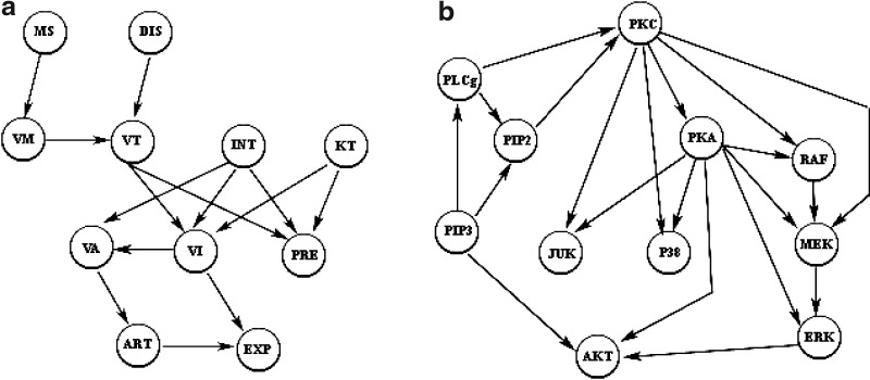
In the present study, we use a subset of the ALARM (A Logical Alarm Reduction Mechanism) network (Beinlich et al., 1989), which is composed of 11 discrete variables and 14 directed edges as shown in Figure 1a, to generate a synthetic dataset. The conditional probability tables of all the variables in the graph are integrated from the original ALARM network definition. After data generation, we introduce noise into the data by randomly changing each node's value with a fixed probability. The resulting data consists of 100 datasets, and each dataset contains the expression levels for all the variables, among which 20% are configured to be random noise. We generate prior knowledge by randomly picking 50% direct links and various amounts of orderings from the structure given in Figure 1a. The data and prior knowledge are then used to test the model performance. This procedure is repeated multiple times to examine the general effects of prior knowledge on model performance.
FIG. 1.
True network structures: (a) Subgraph of the ALARM network. (b) Schematic of a RAF signaling pathway.
3.2. Real biological data with artificial prior knowledge
We also use the biological data for the RAF signaling pathway, whose schematic pathway structure is shown in Figure 1b. This data is from an intracellular multicolor flow cytometry experiment described in Sachs et al. (2005). In this experiment, quantities of all 11 phosphorylated proteins and phospholipids from the RAF signaling pathway are detected simultaneously under different perturbation conditions.
The data is discretized following an information-preserving discretization method developed by Hartemink (2001), which takes into account variable correlations. The final data we produced consists of 100 datasets in which each contains expression levels for all the molecules. A similar approach as described in Section 3.1 is used on the baseline network structure shown in Figure 1b to derive the prior knowledge for evaluating our model performance.
3.3. Prior knowledge derived from public databases
In both previous cases, generation of the prior knowledge depends on a known network structure. This is reasonable for evaluation purposes. However, a different approach is necessary for model-learning studies in which the network structure itself is aimed to be resolved. To address this issue, we devised an approach to identify prior knowledge regarding direct molecular links and orderings from Kyoto Encyclopedia of Genes and Genomes (KEGG) pathways and Gene Ontology (GO) annotation databases.
We retrieve direct links prior knowledge by searching interactions between each pair of molecules against the total 201 biological pathways in KEGG database. We assign the prior probability for an interaction as 0.5 if it is not identified in the database, or as  , where x is the frequency of that direct link appearing in the database. We use the parameter c to tune the probability settings. In the present study, we set c to
  so that the prior probability of a direct link is at least 0.9 if that interaction was previously identified and stored in the database. The direct links found with this procedure between molecules in the RAF signaling pathway and their associated probabilities are listed in Table 1.
Table 1.
Direct Link and Ordering Prior Knowledge for RAF Signaling Pathway
| Direct links (pr.) | Orderings (pr.) |
|---|---|
| PLCg → PKC (0.99) | AKT → ERK (0.99) |
| MEK → ERK (0.99) | PKC → ERK (0.99) |
| PKC → RAF (0.99) | PLCg → ERK (0.99) |
| RAF → MEK (0.99) | RAF → ERK (0.99) |
| MEK → JNK (0.9) | PKC → RAF (0.97) |
| PKA → ERK (0.9) | PKC → P38 (0.93) |
| PKC → PKA (0.9) | PKC → AKT (0.92) |
| AKT → P38 (0.92) | |
| PLCg → RAF (0.92) | |
| PLCg → AKT (0.91) | |
| PLCg → P38 (0.9) |
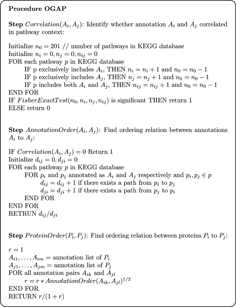
Ordering relations can also be derived from KEGG in a similar manner as discussed above. However, a problem with this approach is that the ordering relationships from KEGG may make sense only in some specific biological contexts and not necessarily in the network that one is interested in constructing. To address this concern, we apply a key helpful observation about molecular ordering; that is, biological signal transduction will, in general, favor a direction from one cellular component to another. For example, in a signal transduction pathway, information is more likely to transfer from a membrane-bound receptor to a transcription factor, which is located in cytoplasm and/or nucleus rather than the other way around. Based on this observation, we design a procedure called ordering from GO annotation and pathways (OGAP) to derive molecular orderings in a biological network. Essentially, this procedure first derives ordering relations of cellular components in biological networks, and then uses this information together with GO annotation of each molecule to find molecular orderings. The specifics of this procedure are presented as pseudo-code in Figure 2.
FIG. 2.
The pseudo-code of the OGAP algorithm.
The OGAP procedure consists of three steps. The first step, Correlation, identifies cellular component pairs that tend to coexist in the same biological pathway. The second step, AnnotationOrder, computes the ordering for each pair of cellular components that pass the test in the first step. Finally, the third step, ProteinOrder, uses the annotation ordering information to derive the probabilities of molecular ordering relations.
We applied the OGAP procedure to all the protein pairs in human KEGG pathways and found out 5% of them have ordering probabilities larger than 0.9. Using this as the threshold, we identified totally 11 protein pairs from the RAF signaling pathway showing ordering relations, as listed in Table 1. Comparing them with the pathway shown in Figure 1b, we can see that 9 out of 11 orderings are consistent with the pathway structure, 1 contradicts, and 1 is missing. The probability values in Table 1 are used in Equation (1) to compute the prior probability of a given network structure.
4. Results
4.1. Model learning with synthetic data
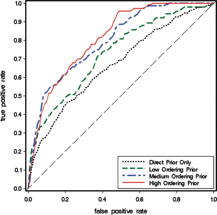
We first examine the performance of our Bayesian network model on the synthetic data and artificial prior knowledge introduced in Section 3.1. In this study, we integrate ≤20% (low), 20%–60% (medium), or ≥60% (high) of ordering relations from Figure 1a as prior knowledge into our Bayesian network model. Figure 3 shows the receiver operating characteristic (ROC) curves from all the model-learning outcomes, where each curve is an average of model outputs from 10 experiments. ROC curves plot true positive rate (i.e.,  ) versus false positive rate (i.e.,
  ).
).
FIG. 3.
ROC curves of Bayesian network models' learning results under different settings.
Figure 3 shows that when ordering relations are included into the model learning, the Bayesian network model performs significantly better, as shown by the larger area under the ROC and the steeper slope at the left side of the curve. Furthermore, when the quantity of the ordering relations continuously increases, the model performance also keeps improving until it reaches a saturation point. This makes sense because the effect of prior knowledge will have a limit. For example, if the prior knowledge already contains orderings from A to B and B to C, then the ordering from A to C is redundant and adding it to the model will have little effect.
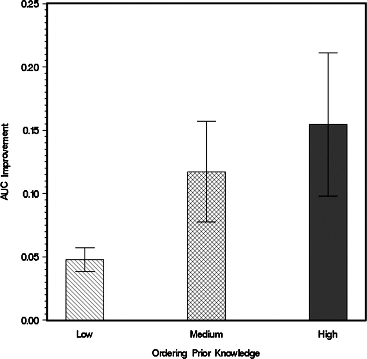
In addition to the average comparison results shown in Figure 3, we also carried out pairwise comparisons between two models with the same data, making one model trained with only direct-edge prior knowledge and the other with additional ordering knowledge beyond direct-edge prior knowledge. The outputs from the two models are compared by their differences in areas under ROC curves (AUC). The results are summarized in a bar chart with 95% confidence interval, as shown in Figure 4. The figure also suggests that addition of prior ordering knowledge would lead to a better model performance, but its effects would be saturated if prior knowledge is continuously added.
FIG. 4.
AUC of Bayesian network models with different abundance of ordering prior knowledge.
4.2. Model learning with real biological data
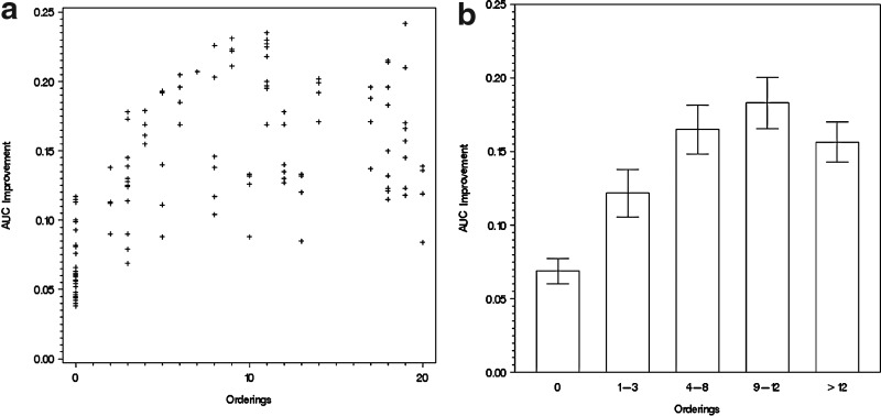
We ran our Bayesian network models on the biological data from the RAF signaling pathway introduced in Section 3.2. Again, we carried out pairwise tests between models with or without randomly picked orderings from the signal transduction pathway, given the same biological data and a fixed set of direct-link prior knowledge. The AUC improvement of their ROC curves are plotted against the quantity of ordering relations, as shown in Figure 5a.
FIG. 5.
AUC improvement given a specific local priori. (a) The horizontal axis indicates the number of ordering relations in prior knowledge, and the vertical axis shows the increase of AUC. (b) The range under each column shows how many ordering relations are included in the model, and the vertical axis is the increase of AUC. Error bars show 95% confidence intervals.
The scatter plot in Figure 5a shows a linear relationship between the AUC improvement and the number of ordering relations when the latter is at a lower level. However, when more ordering relations are supplied into the model, the improvement is saturated, just like Figure 4 with the synthetic data. This pattern can also be seen clearly in Figure 5b, in which all the crosses in Figure 5a are put into different bins for different quantity of ordering relations. In Figure 5a and b, the improvement at x = 0 (i.e., no ordering relations provided) comes from orderings derived from existing direct links. For example, direct links from A to B and B to C imply an ordering from A to C.
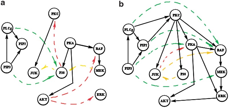
Next, we examine some particular network structures generated by the Bayesian network model. Figure 6 shows two specific network reconstruction results—6a from the model with only direct-link prior knowledge and 6b from the model with additional ordering prior knowledge. We recover, in both cases, the network structures with 90% specificities. It can be seen that with integration of ordering prior knowledge, the Bayesian network model recovers 75% true positive edges (shown by solid arrows) in the signaling pathway, while without that prior knowledge, the percentage drops to 40%. The edges in both networks are color coded according to their consistencies with the RAF signaling pathway. Green, red, and yellow indicate consistent, contradictory, and missing relations in the known network structure, respectively. The results in Figure 6 illustrate that the integration of ordering prior knowledge can help the Bayesian network model recover more true edges and less false edges.
FIG. 6.
RAF signaling pathway reconstruction. (a) Network structure recovered from RAF signaling pathway data and direct-link prior knowledge. (b) Network structure recovered with additional ordering prior knowledge. Black solid edges are true positive edges, and colored dashed edges are false positive edges.
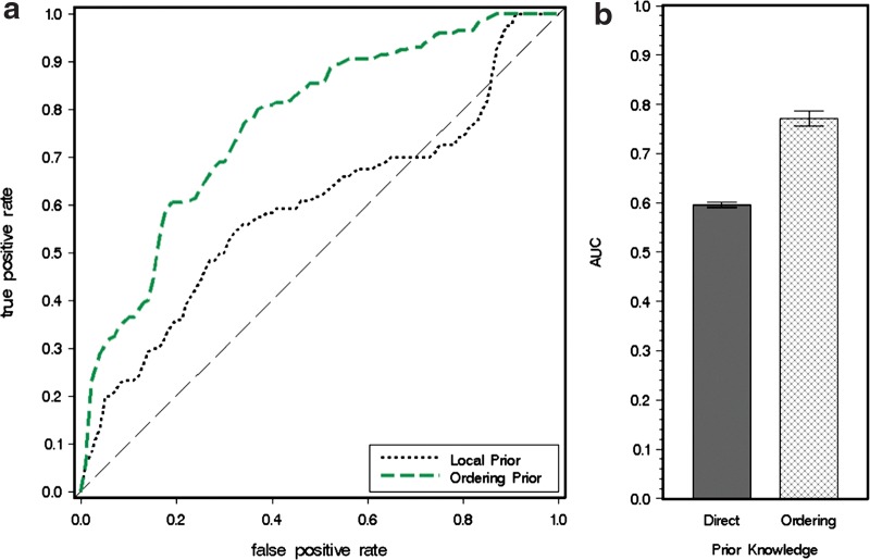
Finally, we discuss the results of using both the flow cytometry data for RAF signaling pathway and the prior knowledge automatically generated from the OGAP process introduced in Section 3.3. Figure 7a shows the average ROC curves from 10 model-learning results. In the figure, we can see that the integration of extra ordering prior knowledge clearly improves the model performance. Figure 7b shows a bar chart of the AUC of ROC curves, which also shows a significant improvement in AUC with the integration of ordering prior knowledge.
FIG. 7.
Model learning results with RAF data and automatically generated prior knowledge. (a) ROC curves of model with and without ordering prior knowledge. (b) Bar chart of AUC. Error bars represent 95% confidence intervals.
5. Conclusions
In the present study, we examined the effects of incorporating ordering prior knowledge on reconstructing a biological network with Bayesian network models. Two contributions of this work are (i) the approach that outlines how to explicitly integrate both direct links and ordering relations as prior knowledge into Bayesian network models, and (ii) the OGAP method that automatically derives ordering relations among biological molecules by analyzing their biological annotations.
In regard to the Bayesian network model, we proposed and demonstrated that the reverse engineering of biological network structures can be improved by integrating direct links and indirect ordering relations known a priori. Each type of prior knowledge is assigned random weights so that the model can adapt itself automatically with given prior knowledge and data. We carried out computational experiments evaluating our methods with both synthetic data and real biological data. We showed that the integration of ordering prior knowledge can significantly improve the sensitivity and specificity of the Bayesian network model and also the fact that the degree of improvement is correlated with the abundance of ordering relations integrated into the model.
In regard to the OGAP method, we aimed to show that the method can derive biological molecule orderings from knowledge resources such as KEGG and GO annotation. Specifically, the orderings of molecules are inferred from their cellular component information in GO annotations and the pathway structures from the KEGG database. We applied this approach to a real biological signaling network and have demonstrated that the method can recover ordering information with reasonable sensitivity and high specificity. This automatically mined information was then used in reverse engineering of a network structure, and we showed that application of such derived information can indeed result in a significant improvement in model learning.
Acknowledgment
This work was supported in part by a grant from NIH/NIGMS, grant no P20 GM65764-04. The authors also thank Dr. David Rowe, Dr. Lynn Kuo, and Dr. Ion Mandoiu for insightful discussions.
Disclosure Statement
The authors declare no competing financial interests exist.
References
- Beinlich I.A. Suermondt H.J. Chavez R.M. Cooper G.F. Technical Report KSL-88-84. Knowledge Systems, AI Laboratory; 1989. The alarm monitoring system: A case study with two probabilistic inference techniques for belief networks. [Google Scholar]
- Cooper G.F. Herskovits E. A Bayesian method for the induction of probabilistic networks from data. Machine Learning. 1992;9:309–347. [Google Scholar]
- Friedman N. Linial M. Nachman I. Using bayesian networks to analyze expression data. Journal of Computational Biology. 2000;7:601–620. doi: 10.1089/106652700750050961. [DOI] [PubMed] [Google Scholar]
- Friedman N. Murphy K.P. Russell S.J. Learning the structure of dynamic probabilistic networks. Proc. Fourteenth Conference on Uncertainty in Artificial Intelligence (UAI'98); 1998. pp. 139–147. [Google Scholar]
- Geier F. Timmer J. Fleck C. Reconstructing gene-regulatory networks from time series, knock-out data, and prior knowledge. BMC Systems Biology. 2007;1:11. doi: 10.1186/1752-0509-1-11. [DOI] [PMC free article] [PubMed] [Google Scholar]
- Gifford D.K. Jaakkola T.S. Using graphical models and genomic expression data to statistically validate models of genetic regulatory networks. Pacific Symposium on Biocomputing. 2001:422–433. doi: 10.1142/9789814447362_0042. [DOI] [PubMed] [Google Scholar]
- Grzegorczyk M. Husmeier D. Edwards K.D. Ghazal P. Millar A.J. Modelling non-stationary gene regulatory processes with a non-homogeneous bayesian network and the allocation sampler. Bioinformatics. 2008;24:2071–2078. doi: 10.1093/bioinformatics/btn367. [DOI] [PubMed] [Google Scholar]
- Hartemink A.J. Principled Computational Methods for the Validation and Discovery of Genetic Regulatory Networks Ph.D. thesis AAI0803410. MIT; Cambridge, MA: 2001. [Google Scholar]
- Hastings W.K. Monte carlo sampling methods using markov chains and their applications. Biometrika. 1970;57:97–109. [Google Scholar]
- Heckerman D. Chickering D.M. Learning bayesian networks: The combination of knowledge and statistical data. Machine Learning. 1995;20:197–243. [Google Scholar]
- Husmeier D. Werhli A.V. Bayesian integration of biological prior knowledge into the reconstruction of gene regulatory networks with Bayesian networks. Computional System Bioinformatics Conf. 2007;6:85–95. [PubMed] [Google Scholar]
- Imoto S. Higuchi T. Goto T. Miyano S. Error tolerant model for incorporating biological knowledge with expression data in estimating gene networks. Statistical Methodology. 2006;3:1–16. [Google Scholar]
- Imoto S. Higuchi T. Goto T. Tashiro K. Kuhara S. Miyano S. Combining microarrays and biological knowledge for estimating gene networks via bayesian networks. Proc. 1st IEEE Computer Society Bioinformatics Conference; 2003. pp. 77–89. [PubMed] [Google Scholar]
- Imoto S. Sunyong K. Goto T. Aburatani S. Tashiro K. Kuhara S. Miyano S. Bayesian network and nonparametric heteroscedastic regression for nonlinear modeling of genetic network. Proc. 1st IEEE Computer Society Bioinformatics Conference; 2002. pp. 219–227. [PubMed] [Google Scholar]
- Kaderali L. Dazert E. Zeuge U. Frese M. Bartenschlager R. Reconstructing signaling pathways from rnai data using probabilistic boolean threshold networks. Bioinformatics. 2009;25:2229–2235. doi: 10.1093/bioinformatics/btp375. [DOI] [PubMed] [Google Scholar]
- Ko Y. Zhai C. Rodriguez-Zas S. Inference of gene pathways using mixture bayesian networks. BMC Systems Biology. 2009;3:54. doi: 10.1186/1752-0509-3-54. [DOI] [PMC free article] [PubMed] [Google Scholar]
- Metropolis N. Rosenbluth A.W. Rosenbluth M.N. Teller A.H. Equation of state calculations by fast computing machines. Journal of Chemical Physics. 1953;21:1087–1092. [Google Scholar]
- Murphy K. Mian S. Technical report, Computer Science Division, University of California; Berkeley, CA: 1999. Modelling gene expression data using dynamic bayesian networks. [Google Scholar]
- Nariai N. Kim S. Imoto S. Miyano S. Using protein-protein interactions for refining gene networks estimated from microarray data by Bayesian networks. Pacific Symposium on Biocomputing. 2004;347:336–347. doi: 10.1142/9789812704856_0032. [DOI] [PubMed] [Google Scholar]
- Pei B. Rowe D.W. Shin D.-G. Reverse engineering of gene regulatory network by integration of prior global gene regulatory information. Proceedings of the 2008 IEEE International Conference on Bioinformatics and Biomedicine; Washington, DC: IEEE Computer Society; 2008. pp. 129–134. [Google Scholar]
- Perrier E. Imoto S. Miyanao S. Finding optimal bayesian network given a super-structure. Journal of Machine Learning Research. 2008;9:2251–2286. [Google Scholar]
- Sachs K. Perez O. Pe'er D. Lauffenburger D.A. Nolan G.P. Causal protein-signaling networks derived from multiparameter single-cell data. Science. 2005;308:523–529. doi: 10.1126/science.1105809. [DOI] [PubMed] [Google Scholar]
- Segal E. Pe'er D. Regev A. Koller D. Friedman N. Learning module networks. Journal of Machine Learning Research. 2005;6:557–588. [Google Scholar]
- Tamada Y. Kim S. Bannai H. Imoto S. Tashiro K. Kuhara S. Miyano S. Estimating gene networks from gene expression data by combining bayesian network model with promoter element detection. Bioinformatics. 2003;19:ii227–ii236. doi: 10.1093/bioinformatics/btg1082. [DOI] [PubMed] [Google Scholar]
- Werhli A.V. Grzegorczyk M. Husmeier D. Comparative evaluation of reverse engineering gene regulatory networks with relevance networks, graphical gaussian models and bayesian networks. Bioinformatics. 2006;22:2523–2531. doi: 10.1093/bioinformatics/btl391. [DOI] [PubMed] [Google Scholar]
- Werhli A.V. Husmeier D. Reconstructing gene regulatory networks with bayesian networks by combining expression data with multiple sources of prior knowledge. Statistical Applications in Genetics and Molecular Biology. 2007;6 doi: 10.2202/1544-6115.1282. Article 15. [DOI] [PubMed] [Google Scholar]


