Optimization-based Inference for Temporally Evolving Networks with Applications in Biology

Abstract

The problem of identifying dynamics of biological networks is of critical importance in order to understand biological systems. In this article, we propose a data-driven inference scheme to identify temporally evolving network representations of genetic networks. In the formulation of the optimization problem, we use an adjacency map as a priori information and define a cost function that both drives the connectivity of the graph to match biological data as well as generates a sparse and robust network at corresponding time intervals. Through simulation studies of simple examples, it is shown that this optimization scheme can help capture the topological change of a biological signaling pathway, and furthermore, might help to understand the structure and dynamics of biological genetic networks.

1. Introduction

Modeling of biological genetic networks has received much recent research attention. Many current data-driven inference algorithms, such as Bayesian network models of genetic networks formed by coding a priori knowledge on the regulatory relationships into probabilistic models (Sachs et al., 2002; Friedman and Koller, 2000; Yu et al., 2004), are limited in their ability to represent temporally evolving dynamics. On the other hand, there are many studies of identification of regulatory networks using deterministic models, such as ordinary differential equations (ODEs), or linear models based on least squares identification (Schmidt et al., 2005; Bansal et al., 2006; Schmidt and Jacobsen, 2004). However, such assumptions about the model structure could be problematic because prejudices are automatically imposed, which then restrict the representation and understanding of biological data. For example, a key assumption of a mass-action kinetics model is that there is a large number of molecules that are homogeneously mixed, an assumption that may fail inside a cell when there are only a few molecules governing the reaction. Therefore, such “theory-driven” modeling requires a good understanding of the dynamics of the signaling pathway. However, often models of biological systems are too complex to understand because of the large number of components involved and the nonlinearity of the reaction or interaction. As a result, the behavior of these systems in general cannot be completely understood from a systems point of view.

On the other hand, logical models like Boolean networks (BNs) seek completely qualitative rather than quantitative models of biological systems. BNs can succeed in capturing high-level phenomena such as activation or deactivation with fewer parameters than their ODE counterpart and can be used to evaluate model structure. However, they cannot capture transient response, only steady state. In spite of this, there are many applications of Boolean networks to modeling and analyzing biological systems, because they are easy to simulate or evaluate, as well as an increase in research activities to address questions arising from biological applications (Sontag et al., 2008; Zou, 2010).

Since a graph is a natural way to represent a biological network, if a system can be abstracted into a graph, it might help to understand the biological network. A graph is a set of vertices that represents states and a set of edges that depicts the relationship or connection between two or more states. A given connectivity or adjacency map is a signed, directed graph GR = (V, E, S) where V is a set of vertices, E is a set of directed edges, and S: E → { − 1, 0, + 1}. For example, e_ij = 1 represents the case in which input node j activates output node i. If input node j inhibits output node i, then e_ij = −1. If input node j does not affect output node i, then e_ij = 0. Also, graphs are well-suited for situations in which there is little prior or explicit knowledge of the dynamics. Moreover, if we can build a graph model to represent biological data, we could escape imposed prejudices from the model structure. There are several graph-mining approaches to biological networks (Alon, 2007; Han et al., 2007). These approaches represent biological networks as graphs, where nodes represent genes and edges represent relationships between each gene, and discover frequent patterns or motifs (Alon, 2007) in these graphs. They focus on structural features of networks, and they can effectively uncover the functional interaction structure of a biological network. Also, these approaches consider time-invariant networks and local or modular behavior of large networks. Recent studies (Chang et al., 2009; Kim et al., 2010) have proposed a concept of a temporal sequence of network motifs in which the motifs change according to the dynamic nature of the biological system and can describe pivotal developmental events that cannot be captured by the static network approach. Chang et al. (2009) develops algorithms for graph-rewriting rules based on machine-learning techniques, which brings complexity issues with analyzing very large graphs (Chang et al., 2009). On the other hand, Kim et al. (2010) applies a temporal sequence of network motifs analysis by reconstructing the active subnetworks (3-node subgraphs).

In this article, we focus our attention on identifying time-varying linear models of sparse biological networks represented as graphs. We develop time-varying linear models, where the model remains constant for a time step or a series of time steps. This can capture dynamics that change over time and can allow the graph at each time step to be sparse.

With this approach in mind, our question becomes how to infer the graph structure from a set of data and how to find the most reasonable model among many possible configurations, since our problem formulation has fewer constraints than theory-driven modeling. We assume a priori information is given as a connectivity map, however, this is not necessary, as the map may include all possible connections in the case of no a priori information. In general, including known information helps to find a more biologically reasonable model. For example, without any a priori information, our algorithm can find the most reasonable model in the sense of minimizing a cost function, but if we include known information as a connectivity map, we find the most reasonable model satisfying the connectivity map. Despite uncertainties about details for a given biological system, we often have reasonable qualitative knowledge about interactions of each gene, so we can use this information as a priori information. In this setting, the model behavior is solely based on this qualitative information, which guarantees biologically reasonable behavior: a sparse and smooth evolving network. We formulate our cost function based on those assumptions. Then, using convex optimization techniques, we find the sparsest time-varying graph consistent with experimental observations (Chang et al., 2011b). Also, the reconstructed graph shows the signal propagation through the sparse network that drives the placement of links and nodes. It might help to uncover the underlying dynamics and how the system dynamics evolve over time.

The rest of this article is organized as follows: Section 2 presents the proposed method related to modeling of biological networks and an optimization problem formulation with simple examples. Section 3 presents an example of the biological network of HER2 over-expressed breast cancer, which has motivated our work. Finally, conclusions are given in Section 4.

2. Method

We define a state vector , the components of which represent concentrations of proteins or states in a biological network, and n_x represents the number of components or states. The evolution of state x(t) can be modeled using an ordinary differential equation (ODE):

(1)

where p is a parameter set. The nonlinear dynamic system (Eq. 1) can be approximated by a linear system based on forming the Jacobian around steady states as shown below:

(2)

A system in the form of Equation (2) can be considered as a weighted, directed graph. In this, A represents connectivity and B represents the sensitivity to parameter variation. If A_ij is zero, node j has no direct effect on node i. Also, if A_ij > 0, node j activates node i. Similarly, if A_ij < 0, node j inhibits node i. In Sontag et al. (2004) and Han et al. (2007), a convex optimization is constructed as follows:

(3)

where represents time-course data set with different stimulations and/or inhibitions, and each X_i represents the matrix form of n_x different components at M different time points Also, represents the set of sensitivities of parameter variation with , and W represents a weighting matrix for specific experiments. Also, k is a given positive constant that represents maximum connectivity, all A_i,j > 0 represent activation edges (node j activates node i), and all A_r,s < 0 represent inhibition edges (node s inhibits node r). Therefore, this approach gives us the optimal static graph map consistent with various experimental data sets.

In this article, we extend this idea to a dynamic graph model. First, we define where represents experimental data or known values (normalized or Booleanized biological data) at time k for 1 ≤ k ≤ N, the components of which represent concentrations or activities in a biological network, n_x is the number of states of X_k, and N is the number of discrete time steps. We define an augmented matrix , which is a function of the dynamic graph G_k where each is a connectivity map at time k for 1 ≤ k ≤ N, which is based on a priori information, or a connectivity map denoted by GR. The augmented matrix satisfies an evolution of the state X_k as X_k = G_kX_k−1. In contrast to previous methodologies for dynamic graph analysis (Chang et al., 2009; Kim et al., 2010), we formulate a convex optimization-based inference method, where we embed the dynamics of a linear time varying representation and enforce sparsity and smooth evolution at corresponding time intervals.

2.1. Dynamic graph (linear time varying system)

The state X_k evolves along with time and constitutes the following linear-time varying system:

(4)

where G_k = g(GR,X_k|X_k−1) is a function of both the connectivity map and time series data. Note that G_k describes how the edge activities evolve over time. For example, for given connectivity map GR, we allow the change of strength of connection to drive our dynamic model consistent with biological system or experimental data. At each time step, only a few edges may evolve based on the relationship between X_k and X_k−1. If all the interactions between each component are properly identified, we can reconstruct the map G_k in terms of the connectivity and strength. For instance, G_k(i, j) = 0.5 represents that node j activates node i with strength 0.5. The strength might be related to the reaction rate and the concentration of other species, demonstrated by the Jacobian of a mass-action kinetics model.

The goal of system identification of biological systems is to infer each G_k for 1 ≤ k ≤ N consistent with both a biological data set χ and a priori information GR. In general, a gene regulation network (GRN) has the following characteristics (Marc et al., 2010):

• 1) Directionality: Regulatory control is directed from regulators to regulated genes.

• 2) Sparsity: Each single gene is controlled by a limited number of other genes, which is small compared to the total gene content (and also to the total number of TFs) of an organism.

• 3) Combinatorial control: The expression of a gene may depend on the joint activity of various regulatory proteins.

Since GRNs have a sparse structure with combinatorial control, we should reconstruct the sparsest graph consistent with experimental observations. We can construct an optimization problem as follows:

(5)

where the second term in the cost function penalizes the cost of adding edges in order to avoid heavy combinatoric computation, A_k is defined as follows:

(6)

and γ is a positive constant. Therefore, A_k enforces the network to be sparse, and thus, the cost function represents a trade-off between reconstruction error and sparsity. Here we define the function g as shown below:

(7)

where ⊕ is defined as a projection operator onto , whose i-th column is a column vector, the components of which are all one if X_k−1(i) is active, which means the state of the i-th element is over the threshold. On the other hand, if X_k−1(i) is nonactive, then the i-th column of MAP is a zero-column vector. Therefore, this projection gives us all possible candidate edges based on both X_k−1 and GR. For example, if x_i at the (k − 1)th step is active, then the i-th column of GR contains the candidate edges. On the other hand, if x_i at (k − 1)th step is not active, we cannot use the i-th column of GR as candidate edges. By using Equation (7), our method generates a sparse network representation without any Lasso-type regressions in Equation (5).

If we implement the optimization problem for every single step as shown in Equation (5), the penalty term for sparsity does not play the role of generating a sparse network but instead uses all possible edges. In other words, distributing signal to all possible nodes (dense network) gives us a lower cost than distributing signal to only a few nodes (sparse network) in our formulation (Eq. 5). We can think about this by considering dynamic programming in optimization. The main idea behind dynamic programming is that, to solve a given problem, we need to solve different parts of the problem (subproblems), then combine the solutions of the subproblem to reach an overall solution in a recursive manner. Similarly, in order to find the sparsest smoothly evolving graph, we need to have a certain connection between every subproblem. For example, when we consider the overall time horizon in Equation (8), the penalty term for sparsity can play a key role in generating a sparse graph structure by connecting the discrete time dynamics at each time step with those at different time steps. Then, we can construct a convex optimization problem for the proposed identification problem as shown below:

(8)

Note that the first term of Equation (8), the summation of ||X_k − G_kX_k−1||, forces the minimization of the reconstruction error for a given dynamical network at time k for 1 ≤ k ≤ N. Also, the second term, the summation of ||G_k − G_k−1||_F, plays the role of realizing a smooth evolution and minimizes the change in network evolution. Finally, with the penalty term ||G₁||_F + ||G_N||_F, which acts as a boundary constraint, we can find the sparsest dynamic graph. We can also arrange and reformulate Equation (8) as follows:

(9)

where and for 1 ≤ k ≥ N. Note that the first term of the cost function in Equation (9) is a reconstruction error cost, and the second term plays the role of connecting each discrete system with another and realizing a smooth evolution of the network by selecting effective edges with inequality constraints.

2.2. Static graph (linear time invariant system)

If we assume that the graph model does not evolve with time (static graph G_k = G), such as with a linear-time invariant system (Han et al., 2007), we can modify the structure of and constraints as shown below for a fixed pattern graph:

(10)

where does not depend on time [compared with G_k = g(GR,X_k|X_k−1) for a linear time varying system]. Note that for a fixed graph structure, the optimal solution represents the average connectivity map (Han et al., 2007).

2.3. Dynamic and static graph

We can compare the dynamic graph and static graph method: the main difference in cost function from dynamic and static graph is the penalty for sparsity as follows:

(11)

(12)

where ΔG_k = G_k+1 − G_k. Also, if we modify the constraint for a dynamic graph similar to the static graph approach, the dynamic graph approach gives us a lower cost than the static graph approach because the structural constraint restricts the degrees of freedom in choosing edges:

(13)

where represents the optimal solution of the dynamic graph approach, and represents the optimal solution of the static graph approach.

2.4. Inhibition edges

Based on our formulation of the optimization problem, we can find the optimal solution that satisfies a trade-off between representation of data (dynamics) and sparsity and smooth evolution. However, the optimal solution does not include any inhibition edges (⊣) because it is not necessary according to our optimization problem as shown in Figure 1. For example, if X is active (1) and Y is not active (0), then there might be two possible cases: X inhibits Y (X ⊣ Y connected, Figure 1 [left]) or no connection between X and Y (Figure 1 [right]). Having no connection would give the lower cost. However, we can handle inhibition edges using Boolean logic as an algebraic constraint as shown below:

(14)

FIG. 1.

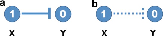
Possible cases for inhibition edge (dash end), where X and Y represent different genes or states; 1 represents activated state and 0 represents deactivated state: (a) inhibition reaction is triggered and (b) inhibition reaction has not occurred.

Also, we extend this algebraic constraint to a normalized state as shown below:

(15)

Consider the simple case shown in Figure 2, in which state X inhibits state Y. Using an algebraic constraint (Eq. 14), we can change the inhibition edge to an activation edge with the new state as shown below:

(16)

FIG. 2.

(a) Inhibition edge ( inhibits ), and (b) modified edge ( activates and the relation between and is defined by Boolean logic or algebraic constraint).

Hence, we extend states if there are inhibition input edges and introduce a diagonal weighting matrix , which makes all species have the same penalty as shown below:

(17)

where represents extended states and . If there exists for a specific state, , and otherwise, .

2.5. Numerical examples

In this section, we consider simple examples to illustrate the proposed inference scheme.

2.5.1. Simple gene network

We first consider a toy example composed of four genes. The a priori information and the snapshot of gene expression are shown in Figure 3. Here, we do not consider state extension for inhibition edges, which means the optimal solution does not include any inhibition edges. By varying the parameter γ, we can sweep out the optimal trade-off curve between the reconstruction error and the sparsity of a solution as shown in Figure 4. We can choose the optimal parameter γ* by the graphical representation: the extreme point γ* on the trade-off between the sparsity and the reconstruction error. Once we fix the parameter γ*, we solve the constrained convex optimization problem (Eq. 29) using a MATLAB-based modeling system for convex optimization (CVX) (Boyd and Vandenberghe, 2004). Figure 5 shows the dynamics of the connectivity graph. We can capture the temporal graph not only in terms of connection but also by strength of the edge. From the optimal graph representations, we could extract how the signaling pathway evolves over time with a systems point of view. Also, we can compare the two approaches: dynamic and static graph approach with average of dynamic graph.

FIG. 3.

(a) A priori connectivity map, where the arrows indicate activation and blunted lines denote inhibition. (b) Snapshots of gene expression from time k = 1 to k = 4 (red or 1: activated states; green or 0: deactivated states).

FIG. 4.

Trade-off curve between the model fitting () and the sparsity () with turning parameter γ.

FIG. 5.

The optimal solution for the example in Section 2.5.1.: the magnitude of each edge represents strength of connection. Also, we compare the results from dynamic and static graph approaches with average of dynamic graph.

2.5.2. Simple gene network with different structure

Here, we add one edge that connects vertex 3 to vertex 2 as shown in Figure 6 and solve the optimization problem again. We can see the difference of the strength of edge 12 (e₁₂) compared with Section 2.5.1 above. Basically, for Section 2.5.1, the optimal graph shows the robust pathway distributing power evenly (e₁₂ and e₁₃ in Figure 5), because both pathways are effective equally. However, for Section 2.5.2, an additional pathway (e₃₂) changes the topology of the graph, which makes the optimal graph choose the more effective or economical path (e₁₃ − e₃₂) in Figure 7. In other words, the optimal solution shows that the strength of e₁₂ decreases because there exists a more effective pathway (e₁₃ − e₃₂).

FIG. 6.

A priori connectivity map with an additional edge (e₃₂), which connects from node 3 to node 2.

FIG 7.

An optimal solution for the example in Section 2.5.2.: an additional pathway (e₃₂) changes the topology of the graph, which makes the optimal graph choose a more effective path (e₁₃ − e₃₂) rather than e₁₂ (for the example in Section 2.5.1., the optimal graph shows distributing power evenly, e₁₂ = e₁₃).

2.6. Extension for the continuous dynamics case

In this article, we infer discrete time dynamics from a set of data with a priori graph structure information and focus on how to find the most reasonable model among many possible configurations. We can extend this idea for the continuous time case. The identification problem has led to a linear quadratic (LQ) optimal control problem with two main penalty functions by which we can match the experimental data with a sparse representation using a priori information of structure (described in the Appendix).

3. Biological Signal Pathway Examples

3.1. p53 Signal pathway

Aswani et al. (2009) proposed a graph-theoretic topological control applied to the p53 signaling pathway. We apply our approach to understand how the controller affects the biological pathway and capture the evolution of the signaling pathway. We define X = [x₁, x₂, x₃, x₄]^T = [x_MDM, x_p53, x_cyclinG, x_c], where x_c is a virtual state that represents the proposed control scheme (actually removing the edge in Aswani et al. 2009):

(18)

Hence, by introducing this virtual state, we have an abstract model of abnormal p53 signaling pathway with controller in Figure 8 (right). Also, we can define GR as follows, based on Figure 9 with extending states, including the state extension due to incorporating the inhibition edges:

(19)

FIG. 8.

(a) An abnormal p53 pathway in Figure 3c in Aswani et al., 2009, and (b) the abstract model that includes the effect of controller.

FIG. 9.

(a,b) Normalized time course plots for the abnormal p53 pathway with controller in Figure 4c in Aswani et al., 2009, and (c,d) dynamic evolution of each edge of abnormal p53 pathway with the controller: the p53 regulates MDM2 similar to the normal p53 pathway by increasing strength of inhibition edge ([p53]-[cyclin G]-[MDM2]).

Here, we normalize the data then apply our algorithm. We can capture the dynamic evolution of the graph in Figure 9. The controller causes the p53 concentrations to increase to higher levels by regulation edge from the murine double minute, an important negative regulator of the p53 tumor suppressor (MDM2) to p53 (also known as protein 53 or tumor protein 53) and causes increased strength of inhibition edge ([p53]-[cyclin G]-[MDM2]). In other words, p53 regulates MDM2 similar to the normal p53 pathway (Aswani et al., 2009). If the controller is not applied again, the strength of edge ([p53]-[cycle G]-[MDM2]) decreases, and the strength of activation edge [p53]-[Controller]-[MDM2] increases. This causes MDM concentrations to increase to higher levels which cause regulation p53 by inhibition edge ([MDM2]-[Controller]-[p53]) similar to the abnormal p53 pathway (Aswani et al., 2009).

We can also apply our algorithm for the normal p53 pathway in order to compare with the abnormal p53 pathway with controller. In a normal p53 pathway, we can consider all possible combinations of both Ras and L26 as two input signals. Here, the basic assumption is that the inhibition reaction is stronger than the activation reaction. Then, we find that the p19 (alternate reading frame of the INK4a/ARF locus (ARF)) mainly regulates MDM2, and it cannot affect MDM2 from p53 through p19 ARF as shown in Figure 10. Hence, we can use the same abstract model in Figure 8 for a normal p53 signaling pathway. The optimal solution shows that the normal p53 cell uses mainly inhibition edges from p53 to MDM2 through cyclin G, which means p53 regulates MDM2, as shown in Figure 11. Therefore, the controller drives the abnormal p53 cell to the normal p53 cell by removing the inhibition edge from MDM2 to p53 as Aswani et al. (2009) proposed.

FIG. 10.

Possible cases for a normal p53 signaling pathway with different combinations of both [Ras] and [L26], where H represents an active state and L represents a nonactive state (Aswani et al., 2009): the p19 ARF mainly regulates MDM2 and it cannot affect MDM2 from p53 through p19 ARF.

FIG. 11.

(a,b) Normalized time course plots for the normal p53 pathway in Figure 4a (Aswani et al., 2009), and (c,d) the dynamic evolution of each edge of the normal p53 pathway: the edge activity shows that the normal p53 cell uses mainly inhibition edges from p53 to MDM2 through cyclin G.

3.2. HER2 overexpressed breast cancer

We are interested in HER2 overexpressed breast cancer, which represents 20–30% of breast cancers. The experimental studies were done for investigating the effects of tyrosine kinase inhibitors (TKIs) on the BT474 and SKBr3 cell lines (Sergina et al., 2007). In this work, short-term effects and long-term effects of applying gefitinib (a TKI) to those cell lines were studied, and important effects of how the cancer cells overcome or escape from the inhibitory effects of TKIs were discovered. The authors in Sergina et al. (2007) showed that HER3 is recruited from the cytoplasm to the cell membrane by vesicular trafficking to increase the triggering signal in order to escape from HER2 inhibition. Also, they tested the effects of vesicular trafficking: when vesicular trafficking was stopped, phospho-HER3 and phospho-Akt did not survive the inhibition of HER2.

We suspect there might be short-term and long-term topological changes because the TKI can inhibit and regulate downstream effectively in the short term, but it cannot regulate for the long term. Therefore, we hypothesize that during the short term, there might be positive negative (PN) feedback (Kim et al., 2007), so the TKI inhibits HER3 effectively. However, for long-term behavior, even a small triggering signal could amplify the phospho-Akt signal, because of positive positive (PP) feedback, which is similar to vesicular trafficking. On the other hand, if the topology does not change, TKI should be able to regulate downstream over the long term even though HER3 is recruited by vesicular trafficking.

We define the a priori map from biological information (Sergina et al., 2007; Amin et al., 2010; Itani et al., 2009), where we include a nucleus model to capture this possible topology change. The behaviors of the nucleus are not yet understood; however, we abstract it with the switch as shown in Figure 12. Basically, there is a fail-safe mechanism, HER2-HER3 signaling, which is buffered so that it is protected against an inhibition of HER2 catalytic activity, and it is driven by the negative regulation of HER3 by Akt (Amin et al., 2010). Also, there is a compensatory mechanism by cross-talk between MAPK and Akt that results in robust activation of this buffering. However, the compensatory buffering prevents apoptotic tumor cell death from occurring as a result of the combined loss of MAPK and Akt signaling (Amin et al., 2010). For example, once a signal is triggered and either MAPK or Akt is high, then the nucleus stays active so MAPK and/or Akt are trying to keep the compensatory buffering. However, once both MAPK and Akt are downregulated, the nucleus is deactivated for all time.

FIG. 12.

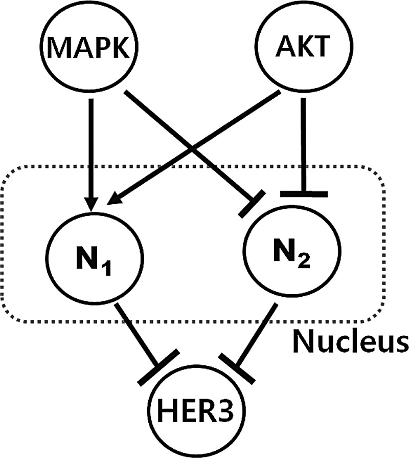
Bifan motif of nucleus, which is two-layered graph with edges from nodes in top- to bottom-layer: there is a fail-safe mechanism, HER2-HER3 signaling, which is buffered so that it is protected against an inhibition of HER2 catalytic activity, and a compensatory mechanism by cross-talk between MAPK and Akt, which results in robust activation of buffering.

We apply the proposed optimization technique and the result is shown in Figure 13 and 14. Here, we use the generated data based on biological experimental data (western blot (Sergina et al., 2007; Amin et al., 2010). By applying the proposed method, we find that there are three main phases: before TKI is introduced (triggering network), right after TKI is introduced (short-term), and long-term behavior after TKI is introduced. We can capture the topology change of the biological network: for the initial stage (Fig. 14a), the signal is triggered and propagated along activation edges. After TKI is introduced, downstream components such as phospho-HER3, PI3K, Akt, and MAPK are regulated because TKI inhibits and regulates downstream components. Moreover, the biological network shows PN feedback, which effectively modulates signal responses. Finally, for long-term behavior, even if a small triggering signal is introduced (because of TKI inhibition, step 17–step 20), the downstream components are not regulated but are activated because the biological network evolves to PP feedback, which induces a slower but amplified signal response and enhances bi-stability.

FIG. 13.

The upper two panels show the normalized biological data and the assumed nucleus level. The lower panels show the strength of the downstream edges. For example, the edge connecting HER23 to MAPK (middle panel) is activated from step 4 to step 9 but deactivated from step 9 to 18.

FIG. 14.

(a) Signal is triggered and propagated along activation edges; (b) after TKI is introduced (short term), downstream components such as phospo- HER3, PI3K, Akt, and MAPK are regulated because TKI inhibits and regulates downstream components (positive negative feedback); and (c) for long-term behavior, even though a small triggering signal is introduced, the downstream components are not regulated but are activated because the biological network evolves to positive positive feedback (gray: not triggered edge; red: activation edge; blue: inhibition edge; light red/blue: deactivated edges after once activated).

4. Conclusion

In this article, we have proposed a data-driven inference scheme in order to understand and identify a model for temporally evolving biological networks. The inference problem has led to a convex optimization problem with two main penalty functions of sparsity and reconstruction error using a priori information of structure. We show through examples that the proposed schemes can be useful to capture the dynamic evolution of the network and understand the biological system with a systems point of view. We use this algorithm to study a breast cancer signaling pathway to help understand short-term and long-term behaviors.

5. Appendix (Continuous Case)

Here, we extend the proposed scheme for the continuous time case. As we mentioned earlier, since a graph model is a natural way to represent a biological signal pathway, it doesn't require any constraints on dynamics such as mass-action kinetics or Hill function representations used in ODE models. Also, many different measurement techniques are developed that allow us continuous data acquisitions. Therefore, the inference scheme for the continuous case can be useful to build models with fine-sampled data set and identify general systems using graphical representation.

5.1. Problem statement

We define a state vector , the components of which represent concentrations of proteins or states in a biological network. It is assumed that the state of the network evolves over time and this evolution of state x(t) can usually be modeled using an ODE:

(20)

where p is a parameter set. As we mentioned in this article, many studies in systems biology impose a structure on f (ċ), such as mass-action kinetics or Hill function dynamics, and identify parameters using least-square criteria. However, we are interested in finding the discrete time-varying influence map that can be formulated as a discrete time-varying linear system. Here, we basically extend this idea for the continuous case. The nonlinear dynamic system (Eq. 20) can be approximated by a time-varying linear system based on forming the Jacobian around steady states as shown below:

(21)

where we assume there is no parameter variation (δp = 0). A system in the form of Equation (21) can be considered as a temporally evolving weighted directed graph. Then, G(t) is a time-varying adjacency matrix, or influence matrix, of dimension n × n, which describes the temporal evolution of the edges with strength change. In general, G(t) is a sparse matrix (Marc et al., 2010):

(22)

where G_i,j(t) is nonzero if there exists a direct connection between node j (input node) and node i (output node). Otherwise, G_i,j(t) is zero.

Definition. Let G(t) be a time-varying adjacency matrix that represents a dynamic graph with n nodes and k edges, where k is the number of candidate edges from a priori information. The component of G(t), denoted e(t) = comp(G(t)), is a k × 1 vector whose elements are the nonzero entries of G(t).

Example. Consider the dynamic graph shown in above Figure A1. Following the conventions introduced above, the corresponding adjacency matrix G(t) has the form:

(23)

FIG. A1.

A simple graph model.

Its component e(t) is constructed by extracting the nonzero elements from each column, which produces the vector:

(24)

Using e(t), we can reformulate Equation (21) as follows (for example, n = 4, k = 5):

(25)

where is a linear function of x, which can be constructed from a priori information, representing possible influence modes of biological networks. For example, the first mode, [0 0 x₁ 0]^T in Equation (25), shows that node 1 activates node 3 (i.e., ). Also, each e_i(t) represents a time-varying coefficient or an activity of i-th mode . Therefore, we can assign the network topology by adding edges, for example, if there are suspicious interactions among nodes.

In order to find all e_i(t), which drive our system dynamics with influence modes, we formulate a linear quadratic (LQ) optimal control problem, as a regulation problem (x(t) → x_d(t)) with control inputs both e(t) and . Once we solve the LQ problem, e_i(t)* shows the optimal activity or sequence of each mode over time, which drives our dynamic system to match biological data.

5.2. Time varying linear system

In order to formulate the LQ optimal control problem, we define the controlled system as follows:

(26)

and the optimal control is sought to minimize the quadratic performance index as follows:

(27)

where S₁, Q₁ and Q₂ are positive semidefinite matrices and R is a positive definite matrix. The LQ problem as formulated above is concerned with tracking of the desired trajectory (x_d(t), biological data). In the performance index J, the first term penalizes the deviation of x(t_f) from the desired trajectory at the final time. Inside the integral, the first term penalizes the transient deviation of x(t), from the desired trajectory x_d(t), which represents the error dynamics. The second penalizes the change of activity of edges (dynamic graph), which attempts to minimize the variation of activity of edges over time (smoothly evolving). Also, the third term penalizes the activities of edges. Therefore, the second and third term attempt to achieve a sparse and smoothly evolving biological network. In order to use a general LQ framework, first we define and . Here, we assume that we know x_d(t) and for 0 ≤ t ≤ t_f because once we have x_d(t) then we can get by using the derivative of a polynomial fitting. We define an (n + k) × 1-dimensional state . Then, the state equation for the enlarged state vector can be formulated as follows:

(28)

where is also a linear function of x. Note that the augmented system is still a linear system because there is no multiplication between A(x) and . Also, the performance index (Eq. 27) can be written as follows:

(29)

The problem is now reformulated as a standard LQ problem with the exception of , which is a singular matrix. However, we are interested in v(t), so the solution of the continuous time LQ problem is given by the state feedback control law as shown below:

(30)

(31)

where and Equation (31) is a Riccati equation (proof in Chang et al., 2011a).

Note that the Riccati Equation (31) includes A(x) term in , yet we can handle this easily by replacing x by x_d. This trick is reasonable because our optimal control input, , drives x(t) to x_d(t) by choosing proper Q₁, Q₂, and R. Otherwise, we would have to solve a two point boundary value problem (TPBVP) by numerical iteration.

Proposition (Chang et al., 2011a). The Riccati equation (31) can be solved by replacing x by x_d, using , which drive x to x_d.

Also, we can evaluate the dynamic graph e(t) by integration:

(32)

Therefore, this proposed LQ optimal control framework allows us to capture pivotal development events and dynamics of the temporally evolving system.

6.3. Numerical example

Numerical examples are illustrated in Chang et al. (2011a).

Acknowledgments

This research was supported by the National Institutes of Health, National Cancer Institute grant U54 CA 112970.

Disclosure Statement

The authors declare that no competing financial interests exist.

References

- Alon U. Network motifs: theory and experimental approaches. Nature Review Genetics. 2007;8:450–461. doi: 10.1038/nrg2102. [DOI] [PubMed] [Google Scholar]
- Amin D.N. Sergina N.A.D., et al. Resiliency and vulnerability in the HER2-HER3 tumorigenic driver. Sci Transl Med. 2010;2:16ra7. doi: 10.1126/scitranslmed.3000389. [DOI] [PMC free article] [PubMed] [Google Scholar]
- Aswani A. Boyd N. Tomlin C. Graph-theoretic topological control of biological genetic networks. Proceedings of the American Control Conference; St. Louis, MO. 2009. [Google Scholar]
- Bansal M. Gatta G.D. Bernardo D. Inference of gene regulatory networks and compound mode of action from time course gene expression profiles. Bioinformatics. 2006;22:815–822. doi: 10.1093/bioinformatics/btl003. [DOI] [PubMed] [Google Scholar]
- Boyd S. Vandenberghe L. Convex Optimization. Cambridge University Press; New York: 2004. [Google Scholar]
- Chang H.Y. Lawrence B.H. Diane J.C. Learning patterns in the dynamics of biological networks. International Conference on Knowledge Discovery and Data Mining archive, Proceedings of the 15th ACM SIGKDD International Conference on Knowledge Discovery and Data Mining; 2009. pp. 977–986. [Google Scholar]
- Chang Y.H. Gray J. Tomlin C. Inference of temporally evolving network dynamics with applications in biological systems. Proceedings of the IEEE Conference on Decision and Control and European Control Conference; Orlando, FL. 2011a. [Google Scholar]
- Chang Y.H. Gray J. Tomlin C. Optimization-based inference for temporally evolving Boolean networks with applications in biology. Proceedings of the American Control Conference; San Francisco, CA. 2011b. [Google Scholar]
- Friedman N. Koller D. A baysian approach to structure discovery in bayesian networks. Machine Learning. 2000;50:95–125. [Google Scholar]
- Han S. Yoon Y. Cho K.H. Inferring biomolecular interaction networks based on convex optimization. Computational Biology and Chemistry. 2007;31:347–354. doi: 10.1016/j.compbiolchem.2007.08.003. [DOI] [PubMed] [Google Scholar]
- Itani S. Gray J. Tomlin C. An ode model for the her2/3-akt signaling pathway in cancers that overexpress her2. Proceedings of the American Control Conference; St. Louis, MO. 2009. [Google Scholar]
- Kim D. Kwon Y.K. Cho K.H. Coupled positive and negative feedback circuits form an essential building block of cellular signaling pathway. BioEssays. 2007;29:85–90. doi: 10.1002/bies.20511. [DOI] [PubMed] [Google Scholar]
- Kim M.S. Kim J.R. Cho K.H. Dynamic network rewiring determines temporal regulatory functions in drosophila melanogaster development processes. Bioessays. 2010;32:505–513. doi: 10.1002/bies.200900169. [DOI] [PubMed] [Google Scholar]
- Marc B.B. Alfredo B. Andrea P., et al. Inference of sparse combinatorial-control networks from gene-expression data: a message passing approach. BMC Bioinformatics. 2010;11:355. doi: 10.1186/1471-2105-11-355. [DOI] [PMC free article] [PubMed] [Google Scholar]
- Sachs K. Gifford D. Jaakkola T. Bayesian network approach to cell signaling pathway modeling. Sci. STKE. 2002;2002:pe38. doi: 10.1126/stke.2002.148.pe38. [DOI] [PubMed] [Google Scholar]
- Schmidt H. Cho K.H. Jacobsen E.W. Identification of small scale biochemical networks based on general type system perturbations. Federation of European Biochemical Societies (FEBS) J. 2005;272:2141–2151. doi: 10.1111/j.1742-4658.2005.04605.x. [DOI] [PubMed] [Google Scholar]
- Schmidt H. Jacobsen E.W. Linear systems approach to analysis of complex dynamic behaviors in biochemical networks. Systems Biology. IEEE Proceeding. 2004;1:149–158. doi: 10.1049/sb:20045015. [DOI] [PubMed] [Google Scholar]
- Sergina N.V. Rausch M. Wang D., et al. Escape from HER family tyrosine kinase inhibitor therapy by the kinase-inactive HER3. Nature. 2007;445:438–441. doi: 10.1038/nature05474. [DOI] [PMC free article] [PubMed] [Google Scholar]
- Sontag E. Kiyatkin A. Kholodenko B. Inferring dynamics architecture of cellular network using time series of gene expression, protein and metabolite data. Bioinformatics. 2004;20:1877–1886. doi: 10.1093/bioinformatics/bth173. [DOI] [PubMed] [Google Scholar]
- Sontag E. Veliz-Cuba A. Laubenbacher R., et al. The effect of negative feedback loops on the dynamics of Boolean networks. Biophysical Journal. 2008;95:518–526. doi: 10.1529/biophysj.107.125021. [DOI] [PMC free article] [PubMed] [Google Scholar]
- Yu J. Smith V.A. Wang P.P., et al. Advances to Bayesian network inference for generating causal networks from observational biological data. Bioinformatics. 2004;20:3594–3603. doi: 10.1093/bioinformatics/bth448. [DOI] [PubMed] [Google Scholar]
- Zou Y.M. Modeling and analyzing complex biological networks incorperating experimental information on both network topology and stable states. Bioinformatics. 2010;26:2037–2041. doi: 10.1093/bioinformatics/btq333. [DOI] [PubMed] [Google Scholar]