A Multi-Compartment Segmentation Framework With Homeomorphic Level Sets

Abstract

The simultaneous segmentation of multiple objects is an important problem in many imaging and computer vision applications. Various extensions of level set segmentation techniques to multiple objects have been proposed; however, no one method maintains object relationships, preserves topology, is computationally efficient, and provides an object-dependent internal and external force capability. In this paper, a framework for segmenting multiple objects that permits different forces to be applied to different boundaries while maintaining object topology and relationships is presented. Because of this framework, the segmentation of multiple objects each with multiple compartments is supported, and no overlaps or vacuums are generated. The computational complexity of this approach is independent of the number of objects to segment, thereby permitting the simultaneous segmentation of a large number of components. The properties of this approach and comparisons to existing methods are shown using a variety of images, both synthetic and real.

1. Introduction

Active contours are extremely popular for image segmentation in computer vision [14, 7]. Those that are implemented using level sets — the so-called geometric deformable models (GDMs) [19] — permit flexible topological changes and yield contours with no self-intersections. In many computer vision applications, it is desirable to simultaneously segment multiple objects in a scene. Although the traditional approach supports the simultaneous segmentation of multiple isolated parts of the same object (by using a single level set with its “inside” in different locations), this does not support the use of different forces for different objects, the preservation of fixed topologies for different objects, or the maintenance of neighborhood relationships between different objects. It may also be desirable to simultaneously segment objects having multiple compartments within them — a multi-object segmentation problem that requires a preservation of both inclusion and geometric relationships between the objects and compartments. Particularly in the segmentation of normal anatomy in biomedical imaging, the above properties are highly desirable.

The extension of GDMs to the segmentation of multiple objects and multi-compartment objects is not straightforward. Difficulties arise because the different forces (internal and/or external) for each object must remain coherent to avoid overlap and vacuum between segmented regions. Similarly, maintaining the topology and relationships during segmentation is a complex and computationally intensive task. Fig. 1 illustrates a simple geometry that actually represents a significant challenge. The three ellipses are to be found in such a way that they remain connected, do not overlap, their outer boundaries conform to the gray level edges, and their inner boundaries are smooth. This is a typical challenge in these multi-compartment problems, and there is no existing method in level set literature solving them.

Figure 1.

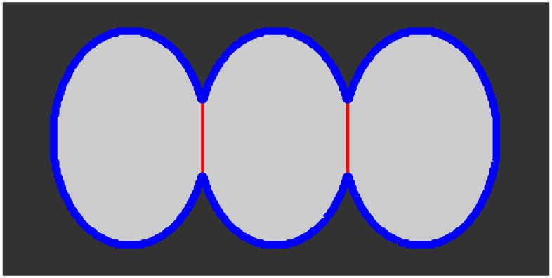
Ellipse example: to segment this image into three ellipses, different forces are needed on the external(blue) and internal(red) boundaries.

In this paper, we present a new framework called multi-compartment geometric deformable model (MGDM), in which the evolution of the level set functions representing any number of objects or compartments is recast into the evolution of just two real-valued functions and two label functions. We emphasize that there is no computational penalty for increasing the number of objects. Conventional level set formulations can be carried out because the two representations are equivalent on a narrow band around the object or compartment boundaries. The topology of objects and the relationships between groups of objects are preserved by using a multi-object simple point constraint instead of their zero level set [17]. The problem of object overlap and vacuum is automatically solved due to the fact that the evolving functions encode directly the partition of the objects. Because two hierarchical labels associated with objects are carried within the computation, it is straightforward to implement object-dependent forces, including different forces on different boundaries that connect specific objects or compartments. The description of MGDM we provide here is valid for two-dimensional images; it is necessary to add a third real-valued function to realize the same benefits in three dimensions.

2. Related Work

A number of approaches have been proposed for the simultaneous segmentation of multiple objects [13, 9, 1, 15, 4, 6, 11, 2, 10, 3, 22]. Most use N level set functions to segment N regions [4, 15, 10, 6, 3], introducing extra coupling forces in order to penalize overlap and vacuum between regions. [22] presents a multi-object curve evolution strategy without involving further numerical parameters. However, these methods do not guarantee no overlap or vacuum and the strict controls of single object’s topology. A probabilistic embedding was also proposed to avoid overlap and vacuum by labelling regions according to their maximum probability [11]. None of these methods guarantee the preservation of the topology of the collection of objects, including their geometric relationships such as common boundaries, although there are methods that guarantee topology preservation of single objects [24, 20].

In [13], Chan and Vese introduced the so-called multiphase level set framework using the Mumford-Shah model [8] to segment multiple objects with no overlap or vacuum. In general, log N level sets are needed to describe N objects and in two dimensions this number may be reduced to two level set functions using the four color theorem. The basic idea of the multi-phase approach is to use a combination of level set functions to represent multiple objects (or components). Although highly attractive from a computational complexity point of view, the multi-phase approach has two key limitations. First, its image-based external force term is limited to region-based forces. Second, its internal forces — a penalty on contour length — apply to the level set functions rather than to the objects. Because of these limitations, anomalous results such as that shown in Fig. 2 can be produced. Here, the two level set functions have achieved level sets with optimal lengths and areas, but the resulting segmentation of the left-most ellipse is clearly wrong, and would not have resulted if the boundary length penalty had been applied to the objects rather than the level set functions. We also note that because of these limitations, specific forces for different regions and different parts of the same region cannot be used in the multi-phase framework.

Figure 2.

Multi-phase segmentation counterexample: a) two level sets obtained with the multi-phase framework, b) the segmentation of the left ellipse.

3. Description of MGDM

Our multi-compartment geometric deformable model (MGDM) is designed to implement the most general multi-object level set deformable model without having to explicitly evolve and maintain all the level sets. In this section, we start by describing an alternate representation of multiple objects that requires maintenance of only four functions. These functions are shown to be equivalent to the original level set functions in their narrow bands provided that there is no point in the image domain touching more than three objects. We then show how an evolution of these four functions can be undertaken to solve the original multi-object level set problem as well as maintaining object topologies and relationships.

3.1. Multi-object Representation

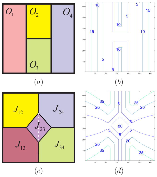
Let Ω ⊂ ℜ² be an image domain in which N regions (objects), O₁, O₂, … O_N, are to be segmented. These objects do not intersect except on their boundaries and their union comprises the entire domain Ω. The locations of the regions are given by a label function L: Ω ↦ where = {1, 2, …, N}. A domain Ω comprising four objects is depicted in Fig. 3(a). For convenience in relating the MGDM to conventional level set evolution equations, we define N level set functions φ₁, φ₂, …, φ_N as distance functions having positive distances inside the respective region and negative values outside. Likewise, the sum of the forces governing the evolution of φ_i, i = 1, 2, …N will be noted as $f_i\triangleq \frac{\partial {\phi }_i}{\partial t}$, i = 1, 2, …, N.

Figure 3.

Multi-object representation: a) object label function L; b) level sets of ϕ_L; c) joint parts {J_ij}, d) level sets of ϕ_F.

We now define a new multi-object distance function ϕ_L: Ω ↦ ℜ as

$${\varphi }_L=\sum _{i=1}^{N}max\{{\phi }_i,0\}.$$ (1)

This function is nonzero everywhere on Ω except on the boundaries between regions. Simply stated, ϕ_L represents the distance to the nearest boundary, as illustrated in Fig. 3(b).

For any point x ∈ Ω, if we are given the values of the label function and the multi-object distance function, then we are immediately able to recover the value of the level set function of the object x is in. But since we are interested in the evolution of the object boundaries, then we also need to be able to recover the value of the level set function of the neighboring object when x is near a boundary. This motivates the need to look at pairs of objects.

Consider the shared boundary b_ij = ∂(O_i ∩ O_j ) between two adjacent objects O_i and O_j as well as the boundary of their union B_ij = ∂(O_i ∪ O_j ). We define the joint part of O_i and O_j as

$$J_{ij}=\{x\in O_i\cup O_j\mid \underset{y\in b_{ij}}{min}||x-y||<\underset{z\in B_{ij}}{min}||x-z||\},$$ (2)

If x ∈ J_ij, then x is closer to the shared boundary between O_i and O_j than to the boundary of their union. The n(n −1)/2 joint parts of all object pairs partition Ω according to each point’s proximity to shared boundaries, as illustrated in Fig. 3(c). It is noted that joint part of two objects is empty if they have no shared boundary.

In order to know what joint part a point belongs to, it is necessary to store one additional label. We define the label function for the first neighbor as follows:

$$F(x)=j,\text{if}x\in O_i\cap J_{ij},$$ (3)

for all i, j, i ≠ j. With this notation, x is in J_ij if {L(x), F (x)} is equal to {i, j} or {j, i}.

Now consider a point x ∈ J_ij. We define ϕ_F at x as the difference between the distance from x to ∂(O_i ∪ O_j ) and φ_L(x). Using the definition of φ_L in Eq. (1) we can write

$${\varphi }_F=\sum _{i,j=1,i\ne j}^{N}max\{{\phi }_{ij},0\}-max\{{\phi }_i,{\phi }_j,0\},$$ (4)

where φ_ij is the level set function of O_i ∪ O_j. The isocontours of ϕ_F are illustrated in Fig. 3(d). We note that ϕ_F is not to be interpreted as the “multi-object distance function” of the joint part. Rather, it is an artificial function designed for the sole purpose of providing a compact representation from which the required level set functions can be reconstructed, as we explain next.

3.2. Level Set Function Equivalence

In this section, we show that φ₁, φ₂, …, φ_N can be directly computed in a narrow band around their level sets from L, ϕ_L, F, and ϕ_F. The following scenario contains the three cases that must be considered. Let O_j and O_k be two distinct objects neighboring O_i such that O_j and O_k are also neighbors. Let O_m be an object different from O_i, O_j, and O_k. For explanatory purposes, it is convenient to define d_m(x) to be the minimum distance from x to the region O_m. Then from the geometry, it is straightforward to verify that the following function equals the level set function of O_i near its boundary

$${\stackrel{\sim }{\phi }}_i(x)=\{\begin{array}{ll}{\varphi }_L(x),\hfill & x\in O_i;\hfill \\ -{\varphi }_L(x),\hfill & x\in \overline{O_i}\cap J_{ij};\hfill \\ -{\varphi }_L(x)-{\varphi }_F(x),\hfill & x\in \overline{O_i}\cap J_{jk}\text{and}{d}_i(x)<{min}_m{d}_m(x);\hfill \\ \text{unknown},\hfill & \text{otherwise}.\hfill \end{array}$$ (5)

In fact, the region over which φ_i can be directly and exactly computed includes all points inside O_i, and the region outside of O_i extending outward to one half the dimension of its neighboring objects.

Since the unknown values are “far away” from the boundaries that are evolving, we can make the approximation that the level set function value in an unknown area is just −ϕ_L(x) − ϕ_F (x) (the same as the third case). Given this, the three locations of x relative to O_i that are relevant in this definition are determined from the label functions L and F. In fact, Eq. (5) can be rewritten to provide the following expression for the level set function of O_i

$${\phi }_i=\{\begin{array}{ll}{\varphi }_L,\hfill & \text{if}L=i;\hfill \\ -{\varphi }_L,\hfill & \text{if}L\ne i,\text{and}F=i;\hfill \\ -{\varphi }_L-{\varphi }_F,\hfill & \text{if}L\ne i,\text{and}F\ne i.\hfill \end{array}$$ (6)

We emphasize first that this function is a valid level set function and second that it is exactly equal to the original level set function of the object itself and (at least) within a narrow band around the object’s boundary.

In the example of Fig. 3, the value of φ₁ is φ₁(x) = ϕ_L(x) for x ∈ O₁. If $x\in \overline{O_1}\cap J_{12}$, i.e., inside the intersection of both yellow parts in Fig. 3(a) and Fig. 3(c), φ₁(x) = − ϕ_L(x). The same happens for $x\in \overline{O_1}\cap J_{13}$, i.e., the intersection of pink in Fig. 3(c) and green in Fig. 3(a). If $x\in \overline{O_1}\cap J_{23}$ and d₁(x) < d₄(x), i.e. the purple region left of the white dotted line in Fig. 3(c), φ₁(x) = −ϕ_L(x) − ϕ_F(x). Values of φ₁ on the right half of the rectangle cannot be recovered accurately, but they do not affect the evolution in a narrow band scheme.

3.3. Evolution of ϕ_L and L

The relationship between φ_i, i = 1, 2, …, N, φ_ij, i, j = 1, 2, …, N, i ≠ = j and the new functions ϕ_L, ϕ_F, L, F being set, any curve evolution originally applied to φ_i, i = 1, 2, …, N can be transferred to ϕ_L, ϕ_F, L and F. The evolution of ϕ_L and ϕ_F is motivated by the forces of several objects, and the following evolution scheme efficiently encodes the necessary coupling of the level set functions without additional constraint forces.

At the boundary between two objects O_i and O_j, the label of each pixel can only switch between the two regions. Eq. (6) requires the forces applied to φ_i and φ_j to be the opposite of each other; thus, we can write

$$\frac{\partial {\varphi }_L}{\partial t}=\frac{1}{2}(f_i-f_j),$$ (7)

for any point where L = i and F = j. Note that a single image sweep is needed, and the evolution forces for each structure are not computed in the whole image but only in the specific area as defined, unlike the methods using N level set functions.

By definition, ϕ_L ≥ 0. Suppose that during the evolution ${\varphi }_L(x)+\frac{\partial {\varphi }_L}{\partial t}(x)<0$. In this case, L(x) should be exchanged from i to j, and ϕ_L(x) is reset to be |ϕ_L(x)|. However, in order to maintain the topology of the segmentation, we further require x to be a simple point for both objects and any possible group of objects in the vicinity [17].

3.4. Evolution of ϕ_F and F

The evolution of ϕ_F follows the same principles, with the difference that the label for the closest neighbor is unknown. ϕ_F is related to the evolution of F. If L(x) = i and F (x) = j, then x is closest to O_j over all the regions except O_i. Therefore F (x) changes only when another neighbor O_k becomes closer to x ∈ O_i than O_j. In terms of the distance functions, it means φ_k > φ_j, which becomes −ϕ_L − ϕ_F > −ϕ_L according to Eq. (6). Thus, we can define the evolution of ϕ_F as

$$\frac{\partial {\varphi }_F}{\partial t}=\frac{1}{2}(f_j-{max}_{k\ne i,j}{f}_k),$$ (8)

Here, the label of the second closest object k is unknown, so it is necessary to search among all the possible neighbors for the one with the highest increment. However, the strict topology constraints ensure that the new neighbor can only come from the subset of objects neighboring O_i and O_j, namely , which can be computed beforehand from the initial contours. The topology of F should not be constrained, as it may change during the evolution even if the topology of L is fixed.

Finally, the evolution of ϕ_F and ϕ_L are coupled: if F changes from j to k at a given step, then the evolution of ϕ_L should use the updated label of F. Therefore, the evolution algorithm must first evolve ϕ_F and then ϕ_L as detailed below.

4. Algorithm

4.1. Narrow Band Evolution

The basic steps of the algorithm are as follows:

1. Given L, initialize ϕ_L, ϕ_F, and F, and compute ∀i, j = 1, …, N, i ≠ j. Choose ε > 0.

2. ∀x s.t. L(x) = i, F (x) = j and ϕ_L(x) < ε, compute f_j and max_k∈ f_k at x. Compute $\frac{\partial {\varphi }_F}{\partial t}$ using Eq. (8).

3. If ${\varphi }_F+\frac{\partial {\varphi }_F}{\partial t}<0$, set ${\varphi }_F=\mid {\varphi }_F+\frac{\partial {\varphi }_F}{\partial t}\mid$, and update F from j to k̂ = arg max f_k.

4. Compute $\frac{\partial {\varphi }_L}{\partial t}$ using Eq. (7) with the updated F.

5. If ${\varphi }_L+\frac{\partial {\varphi }_L}{\partial t}<0$ and topology constraint allows, switch L and F at x. Update ϕ_L to be $\mid {\varphi }_L+\frac{\partial {\varphi }_L}{\partial t}\mid$.

6. Repeat Steps 2–5 until there is no change to L over a sweep.

As in conventional level set methods, periodic reinitialization [18] of ϕ_L and ϕ_F should be done to prevent level set “packing”.

4.2. Computational Complexity and Storage

The methods in [4, 15, 6, 10] must store N level set functions, whereas MGDM must store only two distance-related functions and two label functions. The multi-phase approach of [13] requires storage of log N level set functions in the piecewise-constant case unless a four color labeling is used.

The computational complexity is reduced thanks to the structure of MGDM. We compare the complexity between MGDM, the multi-phase framework [13], and the methods in [4, 15, 6, 10] using a fast marching initialization [18] and a narrow band evolution in Table 1, where n is the number of grid points along a side, and ε is the narrow band width. If we assume that each region has approximately the same number of pixels, then the initialization complexity for ϕ_L is $O(N{(\frac{n}{N})}^{20}log\frac{n}{N})=O(\frac{n^2}{N}log\frac{n}{N})$. And that for ϕ_F is $O(\frac{N(N-1)}{N}{(\frac{n}{N})}^{2}log\frac{n}{N})=O(n^{2}log\frac{n}{N})$. Thus the overall initialization complexity of our approach is $O(n^{2}log\frac{n}{N})$. The other quantities are easy to derive. The complexity of evolution still depends on the number of mutual neighbors in , which is often unrelated to the total number of objects in practice.

Table 1.

Algorithm Complexity

	Fast Marching Init.	Narrow Band Evol.
N φ methods	O(N n2 log n)	O(εN n)
Multi-phase	O(n2 log n log N )	O(εn log N)
MGDM	$O(n^{2}log\frac{n}{N})$	O(εn)

5. Experiments

In this section, we present several multi-object and multi-compartment experiments including test cases and medical images to show the advantages of MGDM.

In the first experiment, the three ellipse phantom image of Fig. 1 is modified for the comparison between MGDM and the multi-phase model [13]. Essentially our framework can correctly segment the phantom image in Fig. 1; in fact, the blue and red lines are the boundaries of our segmentation result. Further, to compare our approach with the multi-phase model that will not work in this case without a internal boundary, the phantom image is modified so that the three ellipses have different mean intensities. The image is then smoothed with a Gaussian filter and the two methods are run with the same region forces and smoothness term and using the same initialization as shown in Fig. 4(a). Fig. 4(b) shows that MGDM segments three ellipses with a smooth boundary with respect to each ellipse, compared to the multi-phase segmentation result presented in Fig. 2, where the boundary of one of the ellipses is artificially large because the two level sets do not coincide exactly. By construction, MGDM avoids this issue entirely.

Figure 4.

Ellipse experiment: a) initialization, b) result of MGDM.

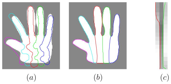
For the second experiment, we apply MGDM to segment the fingers and associated palm of a “hand” image, as shown in Fig. 5. To complicate matters, we introduce wiggles into the initialization [Fig. 5(a)]. In this case, MGDM makes full use of the relationship between regions by applying different levels of smoothing to different parts. Suppose the label for background, thumb, index, middle, ring and little finger are 1 to 6 respectively in this experiment. For the regions with a good contrast between hand intensity and background, i.e., F = 1 or L = 1, we use the region term of [23] and a length smoothing term [21] with a weight of 0.2. For the boundaries between fingers, we impose a stronger smoothing weight of 0.35, and no region term. Fig. 5(b) shows the segmentation result. All the boundaries between fingers are smooth, while the boundaries between fingers and background conform to the region information. The middle and ring fingers are kept separate by the multi-object topology constraint [Fig. 5(c)].

Figure 5.

Hand experiment: a) initialization of the “fingers”; b) final segmentation, c) enlarged region between the middle and ring fingers.

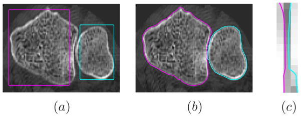
In the following experiments, we apply MGDM to real medical images. Though the main challenge for medical image segmentation is the blurry and noisy source image and the low contrast between objects, MGDM renders satisfactory results as it can combine all existing forces in the level set literature. In the application to carpal bones in Fig. 6, we obtain a satisfying segmentation result with the combination of the GVF [5] external force, the region force of [23] and the curvature smoothing force of [21]. At the same time, the topology constraint prevents the carpal bones from merging [Fig. 6(c)].

Figure 6.

Carpal bone segmentation: a) initialization, b) segmentation result, c) enlarged region of the boundary between two bones.

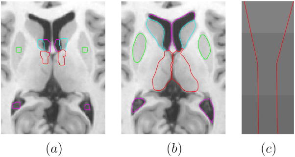
In the segmentation example of Fig. 7, a combination of a balloon force [12] with the membership function from [16] and a curvature smoothing force [21] is used. The joint relationship between ventricles, thalamus and putamen is well maintained, and the triple points among them was dealt with well. Notice that the left and right part of the thalamus does not touch, as enlarged between their boundaries with the background in Fig. 7(c).

Figure 7.

Subcortical segmentation: a) initialization, b) segmentation result, c) enlarged region of the thalamus boundaries.

6. Conclusion

A novel framework to simultaneously segment multiple objects and objects with multiple compartments using level set methods was presented. MGDM guarantees no object overlap and vacuum between objects and can incorporate any existing force in the level set literature while preserving the topology of all objects and groups of objects. As well, different weights can be readily applied to the forces on different objects and on different boundaries of any object thanks to the notion of the joint part. Experiments on simulated and real images validated the framework. Future work will focus on extension to three dimensions and further application to medical images.

References

- 1.Mansouri A, Mitiche A, Vzquez C. Multiregion competition: A level set extension of region competition to multiple region image partitioning. Comp Vis and Imag Underst. 2006;101:137–150. [Google Scholar]
- 2.Tsai A, Wells W, Tempany C, Grimson E, Willsky A. Mutual information in coupled multi-shape model for medical image segmentation. Med Imag Anal. 2004;8:429–445. doi: 10.1016/j.media.2004.01.003. [DOI] [PubMed] [Google Scholar]
- 3.Yezzi A, Tsai A, Willsky A. A fully global approach to image segmentation via coupled curve evolution equations. J of Vis Comm and Imag Repres. 2002;13:195–216. [Google Scholar]
- 4.Samson C, Blanc-Fraud L, Aubert G, Zerubia J. A level set model for image classification. Scale-Space Theories in Computer Vision. 1999:306–317. [Google Scholar]
- 5.Xu C, Prince JL. Snakes, shapes, and gradient vector flow. IEEE Trans Imag Proc. 1998;7:359–369. doi: 10.1109/83.661186. [DOI] [PubMed] [Google Scholar]
- 6.Zimmer C, Olivo-Marin Jean-Christophe. Coupled parametric active contours. IEEE Trans PAMI. 2005;27:1838–1842. doi: 10.1109/TPAMI.2005.214. [DOI] [PubMed] [Google Scholar]
- 7.Cremers D, Rousson M, Deriche R. A review of statistical approaches to level set segmentation: Integrating color, texture, motion and shape. Int’l J Comp Vis. 2007;72:195–215. [Google Scholar]
- 8.Mumford D, Shah J. Optimal approximation by piecewise smooth functions and associated variational problems. Comm Pure Appl Math. 1989;42:577–685. [Google Scholar]
- 9.Angelini E, Song T, Mensh B, Laine A. Multi-phase three-dimensional level set segmentation of brain MRI. MICCAI; 2004. pp. 318–326. [Google Scholar]
- 10.Zhao H, Chan T, Merriman B, Osher S. A variational level set approach to multiphase motion. J of Comp Phys. 1996;127:179–195. [Google Scholar]
- 11.Pohl K, Kikinis R, Wells W. Active mean fields: Solving the mean field approximation in the level set framework. IPMI; 2007. pp. 26–37. [DOI] [PMC free article] [PubMed] [Google Scholar]
- 12.Cohen LD. On active contour models and balloons. CVGIP: Image Understanding. 1991;53:211–218. [Google Scholar]
- 13.Vese L, Chan TF. A multiphase level set framework for image segmentation using the mumford and shah model. Int’l J Comp Vis. 2002;50:271–293. [Google Scholar]
- 14.Kass M, Witkin A, Terzopoulos D. Snakes: Active contour models. Intl J Comp Vision. 1988;1:312–333. [Google Scholar]
- 15.Paragios N, Deriche R. Coupled geodesic active regions for image segmentation: A level set approach. ECCV; 2000. pp. 224–240. [Google Scholar]
- 16.Bazin P, Pham D. Toads: Topology-preserving, anatomy-driven segmentation. ISBI; 2006. pp. 327–330. [Google Scholar]
- 17.Bazin P, Ellingsen L, Pham D. Digital homeomorphisms in deformable registration. IPMI; 2007. pp. 211–222. [DOI] [PubMed] [Google Scholar]
- 18.Malladi R, Sethian JA. Image processing via level set curvature flow. Proc Natl Acad Sci, USA. 1995:7046–7050. doi: 10.1073/pnas.92.15.7046. [DOI] [PMC free article] [PubMed] [Google Scholar]
- 19.Malladi R, Sethian JA, Vemuri BC. Shape modeling with front propagation: A level set approach. IEEE Trans Patt Anal Machine Intell. 1995;17:158–175. [Google Scholar]
- 20.Bischoff S, Kobbelt L. Parameterization-free active contour models with topology control. The Vis Comp. 2004;20:217–228. [Google Scholar]
- 21.Osher S, Sethian J. Fronts propagating with curvature dependent speed: Algorithms based on hamiltonjacobi formulations. Journal of Computational Physics. 1988;79:12–49. [Google Scholar]
- 22.Brox T, Weickert J. Level set segmentation with multiple regions. Image Processing. 2006;15:3213–3218. doi: 10.1109/tip.2006.877481. [DOI] [PubMed] [Google Scholar]
- 23.Chan T, Vese L. Active contours without edges. IEEE Trans Imag Proc. 2001;10:266–277. doi: 10.1109/83.902291. [DOI] [PubMed] [Google Scholar]
- 24.Han X, Xu C, Prince J. A topology preserving level set method for geometric deformable models. IEEE Trans Patt Anal Machine Intell. 2003;25:755–768. [Google Scholar]