Measuring Microsatellite Conservation in Mammalian Evolution with a Phylogenetic Birth–Death Model

Abstract

Microsatellites make up ∼3% of the human genome, and there is increasing evidence that some microsatellites can have important functions and can be conserved by selection. To investigate this conservation, we performed a genome-wide analysis of human microsatellites and measured their conservation using a binary character birth--death model on a mammalian phylogeny. Using a maximum likelihood method to estimate birth and death rates for different types of microsatellites, we show that the rates at which microsatellites are gained and lost in mammals depend on their sequence composition, length, and position in the genome. Additionally, we use a mixture model to account for unequal death rates among microsatellites across the human genome. We use this model to assign a probability-based conservation score to each microsatellite. We found that microsatellites near the transcription start sites of genes are often highly conserved, and that distance from a microsatellite to the nearest transcription start site is a good predictor of the microsatellite conservation score. An analysis of gene ontology terms for genes that contain microsatellites near their transcription start site reveals that regulatory genes involved in growth and development are highly enriched with conserved microsatellites.

Introduction

Microsatellites, also known as short tandem repeats or simple sequence repeats, are composed of short DNA sequences, 1–6 bp in length, repeated in tandem. Microsatellites are useful genetic markers because microsatellite length changes at a rate that is typically orders of magnitude higher than rates of nucleotide substitution (Ellegren 2004; Buschiazzo and Gemmell 2006; Kelkar et al. 2008; Leclercq et al. 2010). Because of this hyper-mutability, microsatellites are traditionally considered to be nonfunctional, “junk” DNA.

Microsatellites make up ∼3% of the human genome (Warren et al. 2008) and some microsatellites are known to perform important genomic functions (Gemayel et al. 2010). For example, microsatellites composed of the motif AC/TG can absorb negative supercoiling through the formation of Z-DNA, which can displace nucleosomes (Liu et al. 2006; Zhang et al. 2006; Xu et al. 2011) and also prevent the formation of potentially hazardous non-B-DNA structures like slipped-strand DNA (Edwards et al. 2009). Microsatellites can also affect RNA secondary structure, altering their binding properties and stability (Riley and Krieger 2009; Meng et al. 2010; Kozlowski et al. 2010).

Some of these functional microsatellites are known to modulate phenotypes as they expand and contract. For example, the expansion of microsatellites that code for proteins are located in untranslated regions (UTRs) can result in neurodegenerative diseases or muscular dystrophy (Fondon et al. 2008). Not all phenotypic changes induced by microsatellite mutations are deleterious, however, and some microsatellites can produce beneficial variation (Fondon et al. 2008; Gemayel et al. 2010). Commonly cited examples of phenotypes modulated by microsatellites are the mating behavior of voles (Hammock and Young 2004) and the morphology of dogs (Fondon and Garner 2004). Additionally, microsatellites in yeast promoters modulate levels of gene expression, and both yeast and human promoters contain relatively high densities of microsatellites (Vinces et al. 2009). These and other microsatellites may be acting as important sources of phenotypic variation (Rando and Verstrepen 2007; Fondon et al. 2008; Hannan 2010), potentially acting as bet-hedging mechanisms (Rando and Verstrepen 2007). Bet-hedging involves stochastically switching phenotypes and can be optimal when the environment is uncertain (Donaldson-Matasci et al. 2010).

To determine which human microsatellites may be of functional significance, one can take a comparative genomics approach and search for highly conserved mammalian microsatellites. Similar approaches have uncovered other types of functional elements in the human genome (Siepel et al. 2005; Guttman et al. 2009). These approaches modeled genome evolution at the nucleotide level and searched for regions in which nucleotide bases have been highly conserved. However, models at the nucleotide level are not easily applied to microsatellites, because nucleotide substitutions are frequently shuffled around, duplicated, or lost as microsatellites expand and contract. The complex history of nucleotide substitutions combined with motif insertions and deletions make alignment of microsatellites very inaccurate. Therefore, typical measures of sequence conservation that involve the rates of nucleotide substitution are not easily applied to microsatellites (Buschiazzo and Gemmell 2010). Although modeling microsatellite evolution at the nucleotide level is possible (Faux et al. 2007), such modeling efforts rely on strong assumptions about sequence evolution that do not apply to the entire genome.

To avoid modeling the complex nucleotide changes that occur in microsatellites, previous studies have considered microsatellites as simply present or absent from a given genome (Buschiazzo and Gemmell 2009, 2010; Mularoni et al. 2010) with the working assumption that the presence of a microsatellite at orthologous positions indicates that the sequence has been conserved. Using this assumption, these approaches have uncovered microsatellites that have been highly conserved across vertebrate genomes (Buschiazzo and Gemmell 2009; Mularoni et al. 2010). For example, Buschiazzo and Gemmell (2009) uncovered microsatellites shared among different vertebrate clades, indicating that these repeats were present in the vertebrate genome prior to the split of these clades 450 Ma. Although that study laid the groundwork for our current analysis, this earlier approach did not strictly measure microsatellite conservation. Rather, it only uncovered a subset of human microsatellite believed to have been present early in vertebrate evolution. Therefore, the work of Buschiazzo and Gemmell (2009) and similar studies (Riley and Krieger 2009; Mularoni et al. 2010) did not attempt to quantify relative conservation of microsatellites.

To provide a measure of microsatellite conservation in mammalian genomes, we conducted a phylogenetic analysis of data from Buschiazzo and Gemmell (2009) that contain virtually every single-copy human microsatellite and its presence or absence in alignments of the human genome with 11 other mammalian genomes. An example alignment of a conserved microsatellite is shown together with the phylogeny used in our analysis (fig. 1). We modeled microsatellite evolution as a birth–death process on this fixed phylogeny, where birth–death indicates the gain–loss of microsatellites at a given locus. The birth–death process is useful here because it reduces the number of possible states for each locus to simply present or absent. Expanding the number of states in our model by including microsatellite length would require a detailed model of microsatellite mutation, and these models can be rather complex (e.g., Calabrese et al. 2001; Kelkar et al. 2011). Ultimately, we are interested in measuring the conservation of microsatellites of any length, and therefore detailed models of microsatellite expansion and contraction may be unnecessarily complex for our purposes.

Fig. 1.—

Conservation of a promoter microsatellite. (A) Phylogeny of mammalian species used in our analyses. Branch lengths are measured in average number of substitutions per 4-fold degenerate site. (B) An example of a highly conserved microsatellite (highlighted in yellow) uncovered by the birth–death mixture model. This GT-motif microsatellite is found ∼800 bp upstream of the insulin growth factor 1 (igf1) transcription start site. (C) Generic examples of other patterns of highly conserved loci. The + and − symbols represent present and absent, respectively.

We used two different birth–death models to better understand microsatellite evolution. Our simplest model assumed that birth and death rates are equal across microsatellite loci and uses the maximum likelihood (ML) method to estimate these rates of microsatellite gain and loss. We found that the rate at which a microsatellite is lost depends on its position, length, and sequence composition. Our second approach used a phylogenetic mixture model that assumes that death rates vary among loci (Yang 1994; Cohen and Pupko 2010). The mixture model allowed us to rank individual microsatellites by their probability of belonging to the lowest death rate class. We used this probability as a measure of microsatellite conservation, and found a clear relationship between distance from a microsatellite to the nearest transcription start site and that microsatellite's conservation score. We also found that the promoters of genes involved in the development and growth are enriched with highly conserved microsatellites. Our results indicate that the phylogenetic mixture model provides a general framework for measuring microsatellite conservation on a genomic scale.

Materials and Methods

Microsatellite Data

Our data set was obtained from Buschiazzo and Gemmell (2010) and is based on the identification of conserved microsatellites in the publicly available alignment of the human genome against 16 other species (available from the UCSC website at ftp://hgdownload.cse.ucsc.edu/goldenPath/hg18/multiz17way/, last accessed 9 June 2012). Briefly, a microsatellite was considered present in another species if a microsatellite in that species overlapped with the human microsatellite in the alignment (Buschiazzo and Gemmell 2010). Microsatellites in transposable elements were not included in this original analysis, and are thus absent from our data set.

Microsatellites in this set are made of 1–6 bp motifs, and are at least 12 nt in length for mono-, di-, tri-, and tetranucleotide repeats and three perfect repeats for penta- and hexanucleotide repeats. These parameters were based on definition of microsatellites found in the literature (details in Buschiazzo and Gemmell 2006, 2009, 2010). These length thresholds are predicted to have rates of expansion and contraction high enough to be polymorphic within a species (Kelkar et al. 2008). We excluded human microsatellites that were closer than 25 bp to other microsatellites. The distance of 25 bp was initially chosen to allow for the design of unique polymerase chain reaction primers. Additionally, these microsatellites are known to behave differently than simple microsatellites (Varela and Amos 2009) and cannot always be classified by a single motif.

We categorized microsatellites by their length, motif, and functional position (coding, intron, 3′ and 5′-UTR, intergenic) in the human genome, as in Buschiazzo and Gemmell (2010). In our analysis, drawing reasonable conclusions from subsets of the data relies on the assumption that this categorization accurately represents the locus on the rest of the phylogeny. For example, if the human microsatellite is included in a coding region, the locus was categorized as coding and we assumed that this categorization was, for the most part, valid across the phylogeny. Although this assumption is not entirely accurate, especially for distantly related species, it allowed us to make some inferences about and control for the effect of motif, length, and position on microsatellite conservation.

Some microsatellites overlap the boundaries between two regions. We limited the categorization of these loci to a single position by prioritizing the regions with the longest overlap or, if there was an even overlap between two regions, we used a preferential site localization: coding > 5′-UTR > 3′-UTR > intron > intergenic regions. For example, a microsatellite that evenly spans a coding and intron boundary would be considered coding.

We restricted our analyses to just the 12 mammalian genomes in the data set (fig. 1) to avoid possible complications from genome expansions and duplications that have occurred outside of the mammalian clade and to avoid inaccuracies driven by alignments of distantly related species (Prakash and Tompa 2007; Buschiazzo and Gemmell 2010). Note that these inaccuracies are only significant in nonmammalian alignments (Buschiazzo and Gemmell 2010). We also excluded microsatellites found in human sex chromosomes because, on average, these chromosomes undergo different numbers of replication events per generation than the autosomal chromosomes. Under these restrictions, our data set has a total of 538,964 human microsatellites and records their presence or absence in 11 other aligned mammalian genomes (fig. 1).

Assumed Phylogeny

The 12-species phylogeny with corresponding branch lengths was taken from Miller et al. (2007). This tree was generated using substitutions in 4-fold degenerate sites in coding regions, established as protein-coding by ENCODE (Miller et al. 2007). Because branch lengths were measured in expected number of substitutions per site, our estimated microsatellite birth and death rates are measured in gains and losses per substitution per 4-fold degenerate site. Measuring tree branches using “evolutionary time” allows us to control for variable rates of evolution across branches.

Birth–Death Model with Homogeneous Rates

Starting with n = 12 species and s microsatellite loci, we represented microsatellite absence/presence data as matrix , where , , y_ij∈{0,1}, 0=absence, and 1=presence. We assumed that the matrix columns, corresponding to microsatellite loci, were independent and identically distributed (iid) and that evolution of each microsatellite absence/presence followed a continuous-time Markov chain (CTMC) on the state space {0,1} with infinitesimal generator

where λ and μ are birth and death rates, respectively. This birth–death process starts with some initial distribution at the root of the phylogeny F and proceeds down the phylogeny in such a way that conditional on the absence/presence state of each internal node of F the microsatellites die and get (re)born independently in the two clades descending from this node. We assume that the root distribution is equal to the stationary distribution of the birth–death CTMC: . We then used Felsenstein's pruning algorithm to compute the probability of observing microsatellite absence/presence data at the tips of the phylogeny F for each locus i:

where 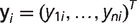(Felsenstein 1981). In our analysis, we considered only microsatellites that are present in the human genome. Following Felsenstein (1992), we corrected this ascertainment bias by conditioning on the event that the human tip in our phylogeny is always in state 1, {h = 1}:

Under our stationarity assumption at the root of the phylogeny, . The assumed iid property of microsatellite loci implies that the likelihood of observing matrix y is

We obtained maximum likelihood estimates of birth and death rates, and , by numerically maximizing the above likelihood with respect to λ and μ using custom C++ and R code. In order to arrive at category-specific estimates (e.g., coding region birth and death rate estimates), we formed a category-specific data matrix y by including into this matrix only loci that belong to a category of interest. We used asymptotic normality of maximum likelihood estimators and the observed Fisher information matrix to construct confidence intervals for birth and death rates.

Birth–Death Mixture Model

To model birth–death rate heterogeneity across microsatellite loci, we used a simplified version of one of the mixture models proposed by Cohen and Pupko (2010), which in turn are slight modifications of the standard phylogenetic gamma mixture model (Yang 1994). Our mixture model postulates that each locus i has a locus-specific death rate , which is obtained by multiplying some unknown baseline rate μ by scaling factor r_i: . The locus-specific scaling factors themselves are iid and gamma distributed:

where α is an unknown shape parameter. In practice, such continuous mixture models are approximated via discretization (Yang 1994). More specifically, we assumed that there were three death rate scaling factors, corresponding to low, medium, and high conservation of microsatellite loci. Then we formed scaling factors r₁,r₂,r₃ by discretizing the distribution. These scaling factors were normalized so that . Using locus probabilities from the homogeneous birth–death model, we wrote the probability of observing locus i under the mixture model as

To correct for the ascertainment bias, we rescaled the above expression by the probability that the human tip of the tree is in state 1:

As before, we formed the likelihood by multiplying locus probabilities,

and maximized this likelihood function to arrive at estimates of birth rate, baseline death rate, and the shape parameter of the gamma distribution: , , and . As before, the maximization was done numerically using custom code. In principle, we could also assume variability in the birth rate as in Cohen and Pupko (2010). However, microsatellites get (re)born very infrequently, making our data much less informative about the birth rate than about the death rate. Motivated by this observation and by the fact that death rate is our main parameter of interest, we chose to keep the birth rate equal across microsatellite loci.

Estimation of birth–death mixture model parameters allowed us to assign each locus i a probability triplet , where

We quantified conservation of microsatellite locus i based on its probability of belonging to the highly conserved class, .

Enrichment Analysis

After estimating parameters of the birth–death mixture model, we chose a cut-off value 0 < c < 1 and classified each locus i as highly conserved if . Suppose this procedure finds x highly conserved loci out of all s loci under consideration. We would like to know if a particular category of microsatellites, A (e.g., loci located in coding regions), are enriched in the set of highly conserved loci. We proceed with standard enrichment analysis based on a hypergeometric distribution (Tavazoie et al. 1999; Huang et al. 2009). Suppose a out of all s loci belong to the category A. Moreover, we find that our set of highly conserved loci contains z < a loci in A. Under the null hypothesis of sampling x loci from s loci uniformly at random, the random number of sampled loci that are in A, X, follows a hypergeometric distribution with parameters s, a, x. We computed the enrichment P value as using the statistical computing environment R (R Development Core Team 2011).

Genomic Regions Enrichment of Annotations Tool

The enrichment of gene ontology terms for highly conserved microsatellites around transcription start sites was done using the Genomic Regions Enrichment of Annotations Tool, version 1.7.0, species assembly hg18 (GREAT; McLean et al. 2010). Briefly, this tool tests for an association between gene ontology terms and genes that contain input sequences, in the form of a genomic position, in their promoter region. We used distances of 2,000 bp from the transcription start site, upstream and downstream, as our “promoter” region. GREAT also provided the distance from all of our microsatellites to the nearest canonical transcription start site. We did not include curated regulatory domains or distal regulatory regions in the analysis.

Linear Regression

We applied a linear regression model to investigate the relationship between our conservation score and other factors associated with each locus. We only examined microsatellites that were at least 5,000 bp from the canonical transcription start site, as provided by GREAT, for a total of 38,432 loci. The covariates used in this analysis were absolute distance to the nearest canonical transcription start site in base pairs, motif (284 different types), length in the human genome, and position in functional region (five different types: coding, 3′ and 5′-UTR, intronic, and intergenic). As our conservation score for each locus, we used the logit of the probability of belonging to the lowest death rate class.

Keeping the identifiability constraints in mind, we estimated 290 regression coefficients in R (R Development Core Team 2011). To overcome the multiple testing problem while testing which of the coefficients are nonzero, we controlled the false discovery rate (FDR) using the R package fdrtool and computed the FDR q value for each regression coefficient (Strimmer 2008).

Results

Global Birth–Death Rate Estimates

Under the assumption of homogeneous rates, the ML estimation of the death rate was 8.59 ± 0.03 deaths per nucleotide substitution at 4-fold degenerate sites per microsatellite (hereafter all rates mentioned use this metric). This result indicates that microsatellites are, on average, lost more rapidly than the rate at which substitutions occur. The ML estimate for birth rate was 0.169 ± 0.03. This is best interpreted as a locus specific rate of (re)birth.

Locus Categorization by Genomic Position and Motif

We categorized microsatellites by their motif and position in the human genome: coding regions, 3′ and 5′-UTR, introns, and intergenic regions (table 2). This categorization allowed us to measure rates for different types of microsatellites. The ML death rate estimates for microsatellites in coding regions, 3′ and 5′-UTR were all relatively low (fig. 2). Microsatellites in these positions are thus more likely to be conserved. In addition, microsatellites in coding regions and 5′-UTR had a relatively high estimated birth rate, indicating an increased rate of gain of microsatellites in these regions.

Table 2.

Enrichment of categories in the highly conserved microsatellite set

	No. of loci	% of loci	No. of cons. loci	% of cons. loci	Enrich. P value
All loci	538,964	100	7,557	100	—
Intronic	225,162	41.8	2,412	31.9	1.0
Intergenic	300,042	55.7	3,315	43.8	1.0
Coding	4,968	0.9	961	12.7	10−772
5′-UTR	2,516	0.4	245	3.2	10−122
3′-UTR	6,276	1.1	624	8.3	10−319
A	104,373	19.3	772	10.2	1.0
AC	91,786	17.0	2,257	29.9	10−168
AT	37,219	6.9	213	2.8	1.0

Note.—The number of loci in each category is given, along with the number of loci found in the highly conserved set (“cons. loci”). Enrichment P values were calculated under a hypergeometric test.

Fig. 2.—

ML birth and death rate estimates for different subsets of the data: coding regions, intronic regions, intergenic regions, 3′ and 5′-UTR, and microsatellites in all of these regions composed of the motifs A, AC, and AT. The point labeled “All loci” is the birth and death estimate for the entire data set. Confidence intervals for these estimates were too narrow to be added to the figure.

In addition, we made motif specific measurements, but microsatellites with different motifs are not necessarily uniformly distributed throughout the genome. For example, many tri- and hexa-nucleotide motif microsatellites are found at a relatively high frequency in coding regions (Li et al. 2004). Therefore, we limit our discussion here to the three most common motifs in our data: A, AT, and AC. Note that motifs were standardized (Kofler et al. 2007; Buschiazzo and Gemmell 2009), so the motif “AC” includes all permutations of the motif, in this case CA, GT, and TG. The majority of these ubiquitous microsatellites are found in stretches of noncoding, presumably nonfunctional regions of the human genome, and thus we assume that the majority of them are nonfunctional (Li et al. 2004). Extensive death rate variation exists among these motifs, indicating a clear motif-specific effect (fig. 2). AC microsatellites had the lowest motif-specific death rate, whereas AT microsatellites had the highest. We excluded coding and UTR microsatellites in this estimate in an attempt to only measure neutral, “non-functional” microsatellites.

Variation was also found among the death rates of less common motifs (data not shown). Rate estimates for less common motifs may be influenced by their relative overabundance in functional genomic regions. Delimiting the effects of sequence constraints in functional regions and effects of motif is thus difficult, and requires a priori knowledge about which regions of the genome are evolving neutrally. Therefore, although our results support the hypothesis that motif does affect the rate at which a microsatellite is lost during evolution (Buschiazzo and Gemmell 2009; Taylor et al. 1999), we did not estimate rates for uncommon motifs.

Locus Categorization by Length

Investigating the relationship between microsatellite conservation and length is not a simple task. Due to their high rate of expansion and contraction, the length of these microsatellites can be highly variable. Each locus has an unknown distribution of lengths for each species, and this distribution may vary significantly between species, and between each species and their ancestors. Therefore, length is not a fixed parameter on the phylogeny.

To better understand how microsatellite length is related to conservation without explicitly modeling microsatellite length evolution, we treat length as a fixed quantity for each locus. We assign each locus a length value equal to the length of the microsatellite in the human genome sequence examined (build36/hg18), and obtain ML birth and death rates for each length value. Our primary intention here to see if microsatellite length in the human genome can serve as a proxy for the effect of microsatellite length, which changes along the phylogeny, on microsatellite birth and death rates. We find that stratifying microsatellites by the human length results in a sensible pattern showing that shorter loci have higher birth and death rates (fig. 3).

Fig. 3.—

ML estimates for microsatellites categorized by their length in the human genome. (A) ML estimates of death rate for each length. (B) ML estimates for birth rate for each length. Error bars on each plot represent 95% confidence intervals. We fix the minimum possible value of the birth rate to 0.

Death rates appear to slightly increase for microsatellites with a length of 60 bp or greater, but we believe these estimates are less meaningful for two reasons. First, there are many more short microsatellites than long microsatellites, and as the sample size decreases with length, uncertainty increases. Second, longer microsatellites have a higher rate of expansion and contraction (Kelkar et al. 2008; Leclercq et al. 2010), and their lengths may be less accurately represented by the length found in the human genome. There are a limited number of microsatellites with lengths longer than 90 bp (1697 loci, 0.3% of the total data), and we did not estimate rates for these lengths.

Mixture Model Results

Under the mixture model, we assumed that death rates follow a discretized gamma distribution, with three rate classes: low, medium, and high. The parameters of our gamma distribution were estimated with the ML method. Table 1 shows that, according to Akaike and Bayesian information criteria, the mixture model is more appropriate for our data than the model with homogeneous rates. This mixture model allowed us to investigate the conservation of individual microsatellites. Microsatellites can be assigned to estimated death rate classes based on their locus-specific probabilities for each class. However, such assignments suppress uncertainty associated with this locus classification. Instead of assigning each locus into a rate class, we examined the relative probabilities of each microsatellite belonging to the three different rate classes. Limiting ourselves to three death rates and a single birth rate allows us to plot the simplex of locus-specific class probabilities (fig. 4). The estimated death rate classes (low, medium, and high) correspond to estimated death rates 5.92, 10.92, and 18.20, respectively. Loci with a high probability of belonging to a single rate are found in the corners of the simplex, whereas loci with approximately equal probabilities of belonging to each rate class are found in the middle.

Table 1.

Model comparsion

	Log Likelihood	AIC	BIC
Homogeneous rates	−716740.79	1433485.58	1433507.97
Mixture model	−708064.18	1416134.36	1416167.95

Note.—We report log likelihood, Akaike Information Criterion (AIC), and Bayesian Information Criterion (BIC) values for the model with homogenous birth–death rates and for the mixture model.

Fig. 4.—

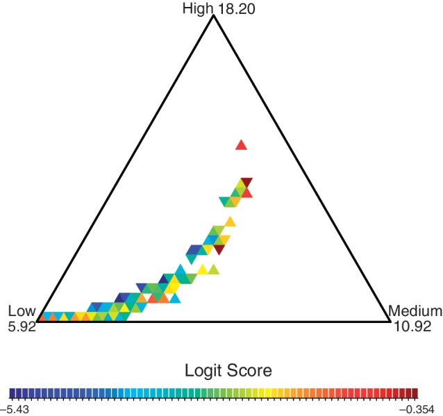
Locus-specific probabilities for the three death rate classes. The color of each triangle represents the frequency of loci that have death rate probabilities within the triangle, with dark red representing the triangles with the highest density of loci. The values of the death rates are indicated at the corners of the simplex. Loci that fall in the middle of the simplex have an equal probability of belonging to each rate class. The color scheme is set on the logit scale, defined as log odds of histogram frequencies. To convert back to the frequency scale, one can use the logistic function (). For example, the boundary logit scale values −5.43 and −0.354 correspond to frequencies 0.0044 and 0.41, respectively.

A large proportion of our loci fell near the center of the simplex plot and did not fit cleanly into any specific death rate class (fig. 4). Although we do not attempt to measure information content per locus, the simplex plot clearly demonstrates that there is limited information about the death rates for many of the microsatellites in our data set, which makes their locus-specific death rates difficult to estimate. Other loci, however, contained sufficient information about their death rates and fell cleanly into the low death rate class. These are the most conserved microsatellites present in the human genome, and are of primary interest to this study. Notice that the ordered nature of death rate classes (low < medium < high) results in a parabolic shape of our simplex histogram.

Highly Conserved Loci

We considered loci with a probability of belonging to the lowest death rate class greater than 99% to be “highly conserved.” According to this criterion, there are 13,600 highly conserved loci representing 2.5% of the total data set. Figure 1 shows some examples of phylogenetic patterns seen at highly conserved loci. These highly conserved loci are significantly enriched with microsatellites in coding, 3′ and 5′-UTR regions (table 2). Microsatellites with the motif AC are also statistically enriched in this set, perhaps reflecting the functional importance of this motif in mammalian genomes (Rothenburg et al. 2001). Only 6% of these highly conserved AC microsatellites are found in regions that encode mRNA.

We are particularly interested in these highly conserved loci as functional elements in gene promoters. Microsatellites have been previously associated with promoters in humans and yeast, both upstream and downstream of the transcription start site (Vinces et al. 2009). To investigate which genes contain highly conserved microsatellites in their promoters, we used the Genomic Regions Enrichment of Annotations Tool (GREAT; McLean et al. 2010), which tests for an association between genomic positions and gene promoters. Using this tool, we examined the association between highly conserved microsatellites and gene promoters, which we defined as 2,000 bp upstream and downstream of the canonical transcription start site.

We found 1,463 genes that contain highly conserved microsatellites in their promoters, ∼8% of the genes examined in the analysis. The results of the gene ontology analysis indicate that these genes are an astonishingly nonrandom sample of the human genome (table 3). We display the results of two tests done by GREAT. The hypergeometric test counts each gene with a microsatellite in its promoter only once, whereas the binomial test counts the total number of base pairs covered by microsatellites in each gene's promoter. Many of these genes encode proteins that are regulatory and are involved in development (see Discussion). Table 3 contains a small subset of the significant gene ontology terms, and the entire list can be found in the Supplementary Material online.

Table 3.

A sample of results with the most significant binomial test values from the online web-tool GREAT (McLean et al. 2010)

Ontology	Category	Binom. FDR Q-value	Binom. fold enrich.	Hyper FDR Q-value	Number of genes found
GO molecular function	Nucleic acid binding	0	9.1	10−17	419
	Protein binding	0	6.8	10−13	843
	Binding	0	6.3	10−13	1167
	Transcription regulator activity	10−305	14	10−44	300
GO biological process	Multicellular organismal development	0	11	10−47	491
	Anatomical structure development	0	11.2	10−47	458
	Developmental process	0	10.4	10−45	515
	System development	0	11.5	10−44	422
	Regulation of cellular biosynthetic process	0	10.3	10−34	450
	Regulation of nucleobase, nucleoside, nucleotide and nucleic acid metabolic process	0	10.4	10−34	449
	Regulation of biosynthetic process	0	10.2	10−34	451
	Regulation of gene expression	0	10.5	10−33	438
	Regulation of nitrogen compound metabolic process	0	10.3	10−33	449
	Regulation of macromolecule biosynthetic process	0	10.5	10−33	430
	Regulation of transcription	0	10.8	10−32	401
Mouse phenotype	Mammalian phenotype	0	8.7	10−50	777
	Nervous system phenotype	0	12.2	10−47	390
	Lethality-prenatal/perinatal	0	12.2	10−44	374
	Growth/size phenotype	0	11	10−40	400

Note.—The test examined enrichment of conserved microsatellites within 2,000 bp of the canonical transcription start site. The binomial false discovery rate (Binom. FDR) Q-values are the result of a test that examines the total coverage of microsatellites in each gene's promoter. The binomial fold enrichment (Binom. Fold Enrich.) represents enrichment of highly conserved loci in promoter regions associated with the gene ontology term. To generate the hypergeometric false discover rate (Hyper FDR) Q-value, genes were counted a single time if their promoters contain at least one microsatellite. In total, all 13,600 microsatellites tested picked 1,463 genes, 8% of the 17,506 genes used in the analysis.

To further investigate the relationship between promoters and microsatellite conservation, we used a linear regression with our conservation score, taken as the logit of the probability of the lowest death rate, as a response and the distance to the nearest transcription start site, in base pairs, as a covariate. To control for other factors that may affect this conservation score, we included three other covariates: the motif type of each locus, the length in the human genome, and the functional category of each locus (coding, 5′-UTR, etc.). Even after controlling for all these factors, distance to the transcription start site is negatively correlated with conservation score (regression coefficient = −0.00016, false discovery q value = 10⁻¹²¹, table 4). This is the second most significant factor in the linear analysis, and remains so even if coding and 5′-UTR microsatellites are removed from the analysis (data not shown). The most significant factor was presence in 3′-UTR. Also, there is a positive correlation seen between microsatellite length and conservation, supporting the trend seen in the ML estimates for length (fig. 3). In addition, all functional categories and many motif types show significant association with our conservation score.

Table 4.

Results of the regression analysis for our conservation score

Covariate	Q-value	Reg. coef.
Intercept: function: 3′-UTR	6.1E-143	1.7
distance to promoter	3.8E-121	−1.6E-04
function: intergenic	6.2E-93	−1.3
function: intron	5.7E-90	−1.2
length	9.5E-82	1.8E-02
motif: AC	2.7E-42	4.7E-01
motif: AT	2.1E-38	−6.9E-01
motif: C	1.5E-31	−1.2
motif: CCG	4.9E-25	4.7E-01
motif: AGC	5.3E-25	6.8E-01
motif: AGG	4.6E-20	4.7E-01
motif: AAT	1.9E-12	−3.9E-01
motif: AATG	6.5E-12	4.4E-01
motif: CCCCGG	1.9E-11	−1.7
motif: ATACCT	6.7E-11	−1.3E+01
motif: CCCCG	1.8E-10	−6.0E-01
motif: AAC	7.3E-10	−3.9E-01
motif: CG	1.8E-07	8.7E-01
motif: AGCCCC	6.8E-07	−1.4
function: coding	1.9E-06	3.8E-01
motif: CCCCCG	6.8E-06	−9.6E-01
motif: CCGCG	8.6E-06	−1.0
motif: AGGGG	9.1E-06	−5.8E-01
motif: ACCCC	1.8E-05	−6.8E-01
motif: AAAAC	2.6E-05	−3.1E-01
motif: ATAG	6.7E-05	−5.6E-01
motif: AGGGC	1.3E-04	−7.7E-01
motif: ACACGC	1.8E-04	2.5
motif: AGGC	2.0E-04	−3.7E-01
motif: CCGG	2.5E-04	−7.4E-01
motif: AGGGGC	2.7E-04	−1.4
motif: ACCCCC	5.7E-04	−8.1E-01
motif: CCCG	8.2E-04	−2.6E-01
motif: CCCGCG	9.4E-04	−1.5
motif: AAAAT	1.0E-03	−3.9E-01
function: 5′ UTR	1.3E-03	−2.6E-01
motif: ATAC	1.5E-03	−3.8E-01
motif: ACG	1.6E-03	1.2
motif: AAAC	2.0E-03	−2.0E-01
motif: AGCGG	2.8E-03	−1.6
motif: AGGCG	3.2E-03	−1.3
motif: CCCGG	3.7E-03	−5.5E-01
motif: AGCCG	4.0E-03	−1.2
motif: AAATT	5.0E-03	−7.1E-01
motif: ACAG	5.2E-03	3.4E-01
motif: ACCC	5.3E-03	−2.6E-01
motif: AATT	5.3E-03	−4.0E-01
motif: AAGCCG	6.0E-03	5.2

Note.—We display regression covariates for which FDR Q-value is <0.01 (second column). The last column shows the corresponding regression coefficients. The adjusted r² for this regression analysis is 0.1588.

Discussion

Modeling microsatellite evolution using simple binary birth–death models allowed us to measure microsatellite conservation without modeling the complex mutational mechanisms prevalent at these loci. We found that microsatellite deaths occur more frequently than nucleotide substitutions, and that microsatellite births appear to be exceedingly rare (fig. 2), supporting the assumption that the presence of a microsatellite in multiple species is the result of sequence conservation, rather than convergent evolution.

These findings disagree with results in Kelkar et al. (2011), where births were found to be more frequent than deaths within primate genomes. This disagreement is likely driven by multiple factors, such as microsatellite birth/death rate variation along mammalian genomes, rate variation accross the tree of mammals, and differences in estimation methodologies employed in the two studies. For example, one difference between our study and the work of Kelkar et al. (2011) is the fact that we did not examine microsatellites in transposable elements, which (Kelkar et al. 2011) showed to be important factors in determining the birth and death rates of microsatellites in primates. In addition, when we used our methodology to estimate birth and death rates only in the primate clade of our mammalian tree, our estimated birth rate became much higher than the original estimate, but still lower than the estimated death rate.

Although evolutionary models at the nucleotide level are the methods of choice for measuring sequence conservation, these models are not easily applied to hypermutable genomic elements which are difficult to align. By simplifying genome alignments into microsatellite presence or absence data, we avoided the need to model the complexities of microsatellite evolution (Buschiazzo and Gemmell 2009). Applying a birth–death model to the simplified alignments allowed us to rank microsatellites by the rate at which they have been lost on our phylogeny, their death rate. We then make the working assumption that microsatellites with the lowest death rates have been conserved because of selection, and not because they have a low mutation rate, although intragenomic variation in rates of nucleotide substitution (e.g., Hardison et al. 2003) may be partially responsible for differences in conservation between microsatellites.

Selection can prevent the loss of a microsatellite, even if the microsatellite itself is neutral. For example, some microsatellites might be conserved simply because they code for amino acid repeats (Faux et al. 2007; Simon and Hancock 2009) that can serve as disordered regions, inducing instability in protein structure (Simon and Hancock 2009). The frequent expansion and contraction of these microsatellites may be selectively neutral, or even slightly deleterious. In this scenario, a microsatellite would be conserved passively, hitchhiking in a functional region simply because mutations within the microsatellite can sometimes interfere with the region's function. Microsatellites with lower rates of expansion and contraction, such as short microsatellites (Kelkar et al. 2008), may be more likely to be found under this neutral selection scenario. These microsatellites are less likely to change length, and therefore less likely to generate potentially deleterious mutations. In fact, selection could preserve the length of these microsatellites, even those with high rates of expansion and contraction, if length changes were highly deleterious.

Other microsatellites, however, might be conserved precisely because of their high mutation rate, which in some cases may provide a selective advantage (Kashi et al. 1997). If these microsatellites are acting to modulate phenotypes (Rando and Verstrepen 2007; Fondon et al. 2008; Gemayel et al. 2010) and microsatellites are responsible for some of the “missing heritability” in the human genome (Hannan 2010), then conserved microsatellites may help to explain some of the phenotypic diversity found in humans and other mammals (Buschiazzo and Gemmell 2010; Mularoni et al. 2010).

For example, microsatellites near transcription start sites can modulate levels of gene expression as they expand and contract, and are important sources of variation in yeast gene expression (Vinces et al. 2009). When transcribed in a gene's 5′-UTR, mutations in microsatellites may alter levels of transcription and translation (Riley and Krieger 2009; Meng et al. 2010; Kozlowski et al. 2010). The high density of microsatellites around the transcription start site in the human genome indicates that they may be serving important functions in this region (Vinces et al. 2009). The negative correlation between a microsatellite's conservation score and its distance to the nearest transcription start site supports this hypothesis. These results suggest that microsatellites can have important functions in mammalian gene promoters, and we are preparing in-depth analyses of microsatellite conservation in these regions.

Genes that regulate development often contain multiple highly conserved microsatellites in their promoters (table 3). Many of these regulatory genes are involved in growth, a trait that has significant agricultural importance. If some of these highly conserved promoter microsatellites are modulating body size they may be useful for animal breeding programs. For example, insulin growth factor 1 (igf1), contains a highly conserved microsatellite ∼800 bp upstream of its start site (fig. 1). This microsatellite appears to be a conserved source of variation in growth, as the length of this microsatellite is associated with circulating igf1 levels and/or body size in humans (Rietveld et al. 2004; Sweeney et al. 2005; Akin et al. 2010; Chen et al. 2011), pigs (Estany et al. 2007), and cows (Curi et al. 2005). Highly conserved microsatellites in the promoters of developmental regulators like igf1 may make useful targets for quantitative genetics studies.

Although the birth death model has uncovered many interesting conserved microsatellites, it does not explicitly model the changes in microsatellite length or the accumulation of nucleotide substitutions within the microsatellite. Such a model would not necessarily affect which microsatellites are considered to be conserved. It would, however, provide further insight into how microsatellite length and nucleotide substitutions might relate to microsatellite death on the mammalian phylogeny.

Recently, a detailed model of microsatellite birth and death in primates indicates that both length change and nucleotide substitution are responsible for microsatellites births and deaths (Kelkar et al. 2011). For short microsatellites, nucleotide substitutions are the more frequent cause of births and deaths (Kelkar et al. 2011). Therefore, the higher observed birth and death rates for short microsatellites seen in figure 3 are likely due to the fact that short microsatellites are fewer substitutions away from nonmicrosatellite sequences. However, without modeling microsatellite evolution at the nucleotide level, we cannot determine the relationship between nucleotide substitution, length change, and microsatellite conservation in our results. Therefore, we recommend interpreting results displayed in figure 3 with caution, as microsatellite length in the human genome provides only a very rough approximation of the length effect on microsatellite conservation.

Another limitation of our model comes from the way that we examine other factors affecting our rate estimates, such as motif or position. We used a two-stage approach; first estimate the rates, then examine how these factors may affect these rates. This could be done in one stage, in which the log of the death rate is taken as a linear combination of predictive factors, and ML is then used to infer rates parameters of this generalized linear model. If this approach were used in the mixture model, it would provide locus-specific rate estimates conditional on various predictive factors. This approach would be more computationally demanding, but would obtain more accurate (conditional) rate measurements.

An additional limitation of our approach comes from the data. The ability of a mixture model to detect microsatellite conservation is restricted by the amount of information in the data. In our results, locus-specific death rate class assignments were uncertain for many of the loci examined; many loci had an approximately equal probability of belonging to any specific death rate class (fig. 4). The accuracy of locus-specific assignments should increase if we add more species to the analysis. A larger data set will also enable us to use more sophisticated mixture models to accurately estimate locus-specific microsatellite death rates (Yang et al. 2005).

Conclusion

We performed the first statistically rigorous analysis of human microsatellite conservation on a mammalian phylogeny. The simplicity of the birth–death models allows us to make measurements of microsatellite conservation on a genome-wide scale. Although more complicated methods could have been used, our approach has nevertheless uncovered some interesting patterns related to microsatellite evolution. We hope this and future work on conserved microsatellites will help shed light on the functional importance of these hypermutable elements. Our publicly available results (see Supplementary Material online) include the location, motif, and conservation score for each microsatellite. These results can be used to select candidate microsatellites to be used in association studies.

Supplementary Material

We have made our data set publicly available at www.stat.washington.edu/vminin/sawaya2011_supp/, last accessed 9 June 2012. The full list of results from GREAT can also be found there. The software is available from https://github.com/dnlennonpu01/mcsmac, last accessed 9 June 2012.

Literature Cited

- Akin F, Turgut S, Cirak B, Kursunluoglu R. IGF(CA)19 and IGFBP-3-202A/C gene polymorphism in patients with acromegaly. Growth Horm IGF Res. 2010;20:399–403. doi: 10.1016/j.ghir.2010.09.001. [DOI] [PubMed] [Google Scholar]
- Buschiazzo E, Gemmell NJ. The rise, fall and renaissance of microsatellites in eukaryotic genomes. Bioessays. 2006;28:1040–1050. doi: 10.1002/bies.20470. [DOI] [PubMed] [Google Scholar]
- Buschiazzo E, Gemmell NJ. Evolution and phylogenetic significance of platypus microsatellites conserved in mammalian and other vertebrate genomes. Aust J Zoology. 2009;57:175–184. [Google Scholar]
- Buschiazzo E, Gemmell NJ. Conservation of human microsatellites across 450 million years of evolution. Genome Biol Evol. 2010;2:153–165. doi: 10.1093/gbe/evq007. [DOI] [PMC free article] [PubMed] [Google Scholar]
- Calabrese PP, Durrett RT, Aquadro CF. Dynamics of microsatellite divergence under stepwise mutation and proportional slippage/point mutation models. Genetics. 2001;159:839–852. doi: 10.1093/genetics/159.2.839. [DOI] [PMC free article] [PubMed] [Google Scholar]
- Chen HY, et al. Haplotype effect in the IGF1 promoter accounts for the association between microsatellite and serum IGF1 concentration. Clin Endocrinol. 2011;74:520–527. doi: 10.1111/j.1365-2265.2010.03962.x. [DOI] [PubMed] [Google Scholar]
- Cohen O, Pupko T. Inference and characterization of horizontally transferred gene families using stochastic mapping. Mol Biol Evol. 2010;27:703–713. doi: 10.1093/molbev/msp240. [DOI] [PMC free article] [PubMed] [Google Scholar]
- Curi R, Oliveira H, Silveira A, Lopes C. Effects of polymorphic microsatellites in the regulatory region of IGF1 and GHR on growth and carcass traits in beef cattle. Animal Genet. 2005;36:58–62. doi: 10.1111/j.1365-2052.2004.01226.x. [DOI] [PubMed] [Google Scholar]
- Donaldson-Matasci M, Bergstrom C, Lachmann M. The fitness value of information. Oikos. 2010;119:219–230. doi: 10.1111/j.1600-0706.2009.17781.x. [DOI] [PMC free article] [PubMed] [Google Scholar]
- Edwards S, Sirito M, Krahe R, Sinden R. A Z-DNA sequence reduces slipped-strand structure formation in the myotonic dystrophy type 2 (CCTG) x (CAGG) repeat. Proc Nat Acad Sci U S A. 2009;106:3270–3275. doi: 10.1073/pnas.0807699106. [DOI] [PMC free article] [PubMed] [Google Scholar]
- Ellegren H. Microsatellites: simple sequences with complex evolution. Nat Rev Genet. 2004;5:435–445. doi: 10.1038/nrg1348. [DOI] [PubMed] [Google Scholar]
- Estany J, et al. Association of CA repeat polymorphism at intron 1 of insulin-like growth factor (IGF-I) gene with circulating IGF-I concentration, growth, and fatness in swine. Physiol Genomics. 2007;31:236–243. doi: 10.1152/physiolgenomics.00283.2006. [DOI] [PubMed] [Google Scholar]
- Faux NG, et al. RCPdb: an evolutionary classification and codon usage database for repeat-containing proteins. Genome Res. 2007;17:1118–1127. doi: 10.1101/gr.6255407. [DOI] [PMC free article] [PubMed] [Google Scholar]
- Felsenstein J. Evolutionary trees from DNA sequences: a maximum likelihood approach. J Mol Evol. 1981;17:368–376. doi: 10.1007/BF01734359. [DOI] [PubMed] [Google Scholar]
- Felsenstein J. Phylogenies from restriction sites: a maximum-likelihood approach. Evolution. 1992;46:159–173. doi: 10.1111/j.1558-5646.1992.tb01991.x. [DOI] [PubMed] [Google Scholar]
- Fondon JW, Hammock EA, Hannan AJ, King DG. Simple sequence repeats: genetic modulators of brain function and behavior. Trends Neurosci. 2008;31:328–334. doi: 10.1016/j.tins.2008.03.006. [DOI] [PubMed] [Google Scholar]
- Fondon J, Garner H. Molecular origins of rapid and continuous morphological evolution. Proc Nat Acad Sci U S A. . 2004;101:18058–18063. doi: 10.1073/pnas.0408118101. [DOI] [PMC free article] [PubMed] [Google Scholar]
- Gemayel R, Vinces MD, Legendre M, Verstrepen KJ. Variable tandem repeats accelerate evolution of coding and regulatory sequences. Ann Rev Genet. 2010;44:445–477. doi: 10.1146/annurev-genet-072610-155046. [DOI] [PubMed] [Google Scholar]
- Guttman M, et al. Chromatin signature reveals over a thousand highly conserved large non-coding RNAs in mammals. Nature. 2009;458:223–227. doi: 10.1038/nature07672. [DOI] [PMC free article] [PubMed] [Google Scholar]
- Hammock E, Young L. Functional microsatellite polymorphism associated with divergent social structure in vole species. Mol Biol Evol. 2004;21:1057–1063. doi: 10.1093/molbev/msh104. [DOI] [PubMed] [Google Scholar]
- Hannan A. Tandem repeat polymorphisms: modulators of disease susceptibility and candidates for ‘missing heritability’. Trends Genet. 2010;26:59–65. doi: 10.1016/j.tig.2009.11.008. [DOI] [PubMed] [Google Scholar]
- Hardison RC, et al. Covariation in frequencies of substitution, deletion, transposition, and recombination during eutherian evolution. Genome Res. 2003;13:13–26. doi: 10.1101/gr.844103. [DOI] [PMC free article] [PubMed] [Google Scholar]
- Huang D, Sherman B, Lempicki R. Bioinformatics enrichment tools: paths toward the comprehensive functional analysis of large gene lists. Nucleic Acids Res. 2009;37:1–13. doi: 10.1093/nar/gkn923. [DOI] [PMC free article] [PubMed] [Google Scholar]
- Kashi Y, King D, Soller M. Simple sequence repeats as a source of quantitative genetic variation. Trends Genet. 1997;13:74–78. doi: 10.1016/s0168-9525(97)01008-1. [DOI] [PubMed] [Google Scholar]
- Kelkar YD, Eckert KA, Chiaromonte F, Makova KD. A matter of life or death: how microsatellites emerge in and vanish from the human genome. Genome Res. 2011 doi: 10.1101/gr.122937.111. Advance Access published October 12, 2011, doi:10.1101/gr.122937.111. [DOI] [PMC free article] [PubMed] [Google Scholar]
- Kelkar Y, Tyekucheva S, Chiaromonte F, Makova K. The genome-wide determinants of human and chimpanzee microsatellite evolution. Genome Res. 2008;18:30–38. doi: 10.1101/gr.7113408. [DOI] [PMC free article] [PubMed] [Google Scholar]
- Kofler R, Schlotterer C, Lelley T. SciRoKo: a new tool for whole genome microsatellite search and investigation. Bioinformatics. 2007;23:1683–1685. doi: 10.1093/bioinformatics/btm157. [DOI] [PubMed] [Google Scholar]
- Kozlowski P, de Mezer M, Krzyzosiak WJ. Trinucleotide repeats in human genome and exome. Nucleic Acids Res. 2010;38:4027–4039. doi: 10.1093/nar/gkq127. [DOI] [PMC free article] [PubMed] [Google Scholar]
- Leclercq S, Rivals E, Jarne P. DNA slippage occurs at microsatellite loci without minimal threshold length in humans: a comparative genomic approach. Genome Biol Evol. 2010;2:325–335. doi: 10.1093/gbe/evq023. [DOI] [PMC free article] [PubMed] [Google Scholar]
- Li Y, Korol A, Fahima T, Nevo E. Microsatellites within genes: structure, function, and evolution. Mol Biol Evol. 2004;21:991–1007. doi: 10.1093/molbev/msh073. [DOI] [PubMed] [Google Scholar]
- Liu H, Mulholland N, Fu H, Zhao K. Cooperative activity of BRG1 and Z-DNA formation in chromatin remodeling. Mol Cell Biol. 2006;26:2550–2559. doi: 10.1128/MCB.26.7.2550-2559.2006. [DOI] [PMC free article] [PubMed] [Google Scholar]
- McLean CY, et al. GREAT improves functional interpretation of cis-regulatory regions. Nat Biotechnol. 2010;28:495–501. doi: 10.1038/nbt.1630. [DOI] [PMC free article] [PubMed] [Google Scholar]
- Meng Z, Jackson N, Shcherbakov O, Choi H, Blume S. The human IGF1R IRES likely operates through a Shine-Dalgarno-like interaction with the G961 loop (E-site) of the 18S rRNA and is kinetically modulated by a naturally polymorphic polyU loop. J Cell Biochem. 2010;110:531–544. doi: 10.1002/jcb.22569. [DOI] [PMC free article] [PubMed] [Google Scholar]
- Miller W, et al. 28-way vertebrate alignment and conservation track in the UCSC Genome Browser. Genome Res. 2007;17:1797–1808. doi: 10.1101/gr.6761107. [DOI] [PMC free article] [PubMed] [Google Scholar]
- Mularoni L, Ledda A, Toll-Riera M, Alba M. Natural selection drives the accumulation of amino acid tandem repeats in human proteins. Genome Res. 2010;20:745–754. doi: 10.1101/gr.101261.109. [DOI] [PMC free article] [PubMed] [Google Scholar]
- Prakash A, Tompa M. Measuring the accuracy of genome-size multiple alignments. Genome Biol. 2007;8:R124. doi: 10.1186/gb-2007-8-6-r124. [DOI] [PMC free article] [PubMed] [Google Scholar]
- R Development Core Team . R: A Language and Environment for Statistical Computing. Vienna, Austria: R Foundation for Statistical Computing; 2011. [Google Scholar]
- Rando O, Verstrepen K. Timescales of genetic and epigenetic inheritance. Cell. 2007;128:655–668. doi: 10.1016/j.cell.2007.01.023. [DOI] [PubMed] [Google Scholar]
- Rietveld I, et al. A polymorphic CA repeat in the IGF-I gene is associated with gender-specific differences in body height, but has no effect on the secular trend in body height. Clin Endocrinol. 2004;61:195–203. doi: 10.1111/j.1365-2265.2004.02078.x. [DOI] [PubMed] [Google Scholar]
- Riley DE, Krieger JN. UTR dinucleotide simple sequence repeat evolution exhibits recurring patterns including regulatory sequence motif replacements. Gene. 2009;429:80–86. doi: 10.1016/j.gene.2008.09.030. [DOI] [PMC free article] [PubMed] [Google Scholar]
- Rothenburg S, Koch-Nolte F, Haag F. DNA methylation and Z-DNA formation as mediators of quantitative differences in the expression of alleles. Immunol Rev. 2001;184:286–298. doi: 10.1034/j.1600-065x.2001.1840125.x. [DOI] [PubMed] [Google Scholar]
- Siepel A, et al. Evolutionarily conserved elements in vertebrate, insect, worm, and yeast genomes. Genome Res. 2005;15:1034–1050. doi: 10.1101/gr.3715005. [DOI] [PMC free article] [PubMed] [Google Scholar]
- Simon M, Hancock J. Tandem and cryptic amino acid repeats accumulate in disordered regions of proteins. Genome Biol. 2009;10:R59. doi: 10.1186/gb-2009-10-6-r59. [DOI] [PMC free article] [PubMed] [Google Scholar]
- Strimmer K. A unified approach to false discovery rate estimation. BMC Bioinformatics. 2008;9:303. doi: 10.1186/1471-2105-9-303. [DOI] [PMC free article] [PubMed] [Google Scholar]
- Sweeney C, et al. Insulin-like growth factor pathway polymorphisms associated with body size in Hispanic and non-Hispanic white women. Cancer Epidemiol Biomarkers Prev. 2005;14:1802–1809. doi: 10.1158/1055-9965.EPI-05-0149. [DOI] [PubMed] [Google Scholar]
- Tavazoie S, Hughes J, Campbell M, Cho R, Church G. Systematic determination of genetic network architecture. Nat Genet. 1999;22:281–285. doi: 10.1038/10343. [DOI] [PubMed] [Google Scholar]
- Taylor J, Durkin J, Breden F. The death of a microsatellite: a phylogenetic perspective on microsatellite interruptions. Mol Biol Evol. 1999;16:567–572. doi: 10.1093/oxfordjournals.molbev.a026138. [DOI] [PubMed] [Google Scholar]
- Varela MA, Amos W. Evidence for nonindependent evolution of adjacent microsatellites in the human genome. J Mol Evol. 2009;68:160–170. doi: 10.1007/s00239-008-9192-3. [DOI] [PubMed] [Google Scholar]
- Vinces MD, Legendre M, Caldara M, Hagihara M, Verstrepen KJ. Unstable tandem repeats in promoters confer transcriptional evolvability. Science. 2009;324:1213–1216. doi: 10.1126/science.1170097. [DOI] [PMC free article] [PubMed] [Google Scholar]
- Warren WC, et al. Genome analysis of the platypus reveals unique signatures of evolution. Nature. 2008;453:175–183. doi: 10.1038/nature06936. [DOI] [PMC free article] [PubMed] [Google Scholar]
- Xu YZ, Thuraisingam T, Marino R, Radzioch D. Recruitment of SWI/SNF complex is required for transcriptional activation of SLC11A1 gene during macrophage differentiation of HL-60 cells. J Biol Chem. 2011;286:12839–12849. doi: 10.1074/jbc.M110.185637. [DOI] [PMC free article] [PubMed] [Google Scholar]
- Yang Z. Maximum likelihood phylogenetic estimation from DNA sequences with variable rates over sites: approximate methods. J Mol Evol. 1994;39:306–314. doi: 10.1007/BF00160154. [DOI] [PubMed] [Google Scholar]
- Yang Z, Wong WSW, Nielsen R. Bayes empirical Bayes inference of amino acid sites under positive selection. Mol Biol Evol. 2005;22:1107–1118. doi: 10.1093/molbev/msi097. [DOI] [PubMed] [Google Scholar]
- Zhang J, et al. BRG1 interacts with Nrf2 to selectively mediate HO-1 induction in response to oxidative stress. Mol Cell Biol. 2006;26:7942–7952. doi: 10.1128/MCB.00700-06. [DOI] [PMC free article] [PubMed] [Google Scholar]