Quantification of External Limiting Membrane Disruption Caused by Diabetic Macular Edema from SD-OCT

Abstract

Purpose.

Disruption of external limiting membrane (ELM) integrity on spectral-domain optical coherence tomography (SD-OCT) is associated with lower visual acuity outcomes in patients suffering from diabetic macular edema (DME). However, no automated methods to detect ELM and/or determine its integrity from SD-OCT exist.

Methods.

Sixteen subjects diagnosed with clinically significant DME (CSME) were included and underwent macula-centered SD-OCT (512 × 19 × 496 voxels). Sixteen subjects without retinal thickening and normal acuity were also scanned (200 × 200 × 1024 voxels). Automated quantification of ELM disruption was achieved as follows. First, 11 surfaces were automatically segmented using our standard 3-D graph-search approach, and the subvolume between surface 6 and 11 containing the ELM region was flattened based on the segmented retinal pigment epithelium (RPE) layer. A second, edge-based graph-search surface-detection method segmented the ELM region in close proximity “above” the RPE, and each ELM A-scan was classified as disrupted or nondisrupted based on six texture features in the vicinity of the ELM surface. The vessel silhouettes were considered in the disruption classification process to avoid false detections of ELM disruption.

Results.

In subjects with CSME, large areas of disrupted ELM were present. In normal subjects, ELM was largely intact. The mean and 95% confidence interval (CI) of the detected disruption area volume for normal and CSME subjects were mean_normal = 0.00087 mm³ and CI_normal = (0.00074, 0.00100), and mean_CSME = 0.00461 mm³ and CI_CSME = (0.00347, 0.00576) mm³, respectively.

Conclusions.

In this preliminary study, we were able to show that automated quantification of ELM disruption is feasible and can differentiate continuous ELM in normal subjects from disrupted ELM in subjects with CSME. We have started determining the relationships of quantitative ELM disruption markers to visual outcome in patients undergoing treatment for CSME.

Disruption of the ELM and the photoreceptor inner/outer segment interface in OCT images are seen as markers for potential visual acuity in DME and other retinal disorders. This study describes an automated method for quantifying ELM disruption in normal subjects and patients with DME.

Introduction

Diabetic macular edema (DME) is the primary cause of vision impairment in patients suffering from diabetes.¹,² Typically, abnormal accumulation of advanced glycation end products leads to the disruption of the blood–retinal barrier, causing interstitial fluid accumulation,³ swelling and thickening of the macular layers, and finally damage to central vision.^4,5 The external limiting membrane (ELM) is a structure that separates the inner segments from the outer nuclear layer, where the Müller cells are joined to the photoreceptor cells. The ELM serves as a skeleton to keep the photoreceptors aligned.⁶ The ELM has been hypothesized to maintain a protein balance between the photoreceptor layer (ISL) and the outer nuclear layer (ONL).⁷ Recently, several studies have shown that ELM interruptions visible on spectral-domain optical coherence tomography (SD-OCT) are associated with lower visual acuity outcome in patients with clinically significant DME (CSME).^8–11 Possibly this is because the integrity of the ELM has a critical role in restoration of the photoreceptor microstructures and alignment.^12–14 Earlier reported approaches^15–17 relied on manual tracing of the corresponding surface or on detecting ELM on 2-D B-scans. However, such studies rely on manual interpretation of the state of the ELM, and high intra- and interobserver variabilities are likely. Automated 3-D analysis of the ELM is of high interest because of its potential to elucidate structural abnormalities with minimal variability and possibly predict visual outcomes in DME.

The purpose of the present study was to describe a novel and fully automated method to quantify the 3-D integrity of the ELM in patients with CSME and in normal subjects. This pilot study showing differences between 16 normal controls and 16 CSME patients was included mainly to demonstrate the practical feasibility of the presented methodology and provide preliminary comparisons between these two groups of subjects. Larger studies will follow.

Methods

Subject and Data Collection

Sixteen subjects diagnosed with clinically significant DME based on stereo biomicroscopic examination by retinal specialists underwent macula-centered SD-OCT imaging (Spectralis; 512 × 19 × 496 voxels; Heidelberg Engineering, Vista, CA). SD-OCT scans were also acquired from 16 normal subjects without retinal thickening exhibiting normal acuity (Cirrus; 200 × 200 × 1024 voxels, 6 × 6 × 2 mm³, voxel size 30 × 30 × 2 μm³; Carl Zeiss Meditec, Inc., Dublin, CA). The collection and analysis of image data were approved by the Institutional Review Board of the University of Iowa and adhered to the tenets of the Declaration of Helsinki; written informed consent was obtained from all participants.

ELM Layer Segmentation

The OCT volume was first segmented automatically using our established multilayer graph-search approach,^18–22 yielding 11 surfaces. Once segmented, the subvolume containing the ELM region between surfaces 6 and 11 (region between the outer plexiform layer [OPL] and the ONL) was flattened based on the segmented retinal pigment epithelium (RPE) surface. The ELM is located between surfaces 6 and 7. Due to the abnormality of the data, the layer segmentation on CSME data sets may be problematic for surfaces 7 and 8, while the result for RPE layer is quite robust (see Fig. 1). Therefore, flattening was consistently based on the segmented RPE layer. Subsequently, an edge-based graph-search surface-detection method¹⁸ was employed to segment the ELM layer on this subvolume. It is important to notice that the layer segmentation is based on a graph-search method that has been successfully validated.^18–22 Specifically, for the ELM layer segmentation, the region features (gradient, surface constraints, and anatomic relationship) were effectively integrated into the graph-search cost function to improve the layer segmentation performance.

Figure 1.  .

SD-OCT layer segmentation on a normal and a CSME subject. (a) Central slice from the original raw SD-OCT from a normal subject. (b) Eleven-surface segmentation results for (a). (c) 3-D rendering of the 11-surface segmentation result for (b). (d) Central slice from the original raw SD-OCT from a CSME subject. (e) Eleven-surface segmentation results for (d). (f) 3-D rendering of the 11-surface segmentation result for (e).

ELM Disruption Area Detection

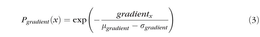
After detection of the ELM layer, each ELM A-scan is classified as disrupted or nondisrupted based on the textural and morphologic properties in the vicinity of the ELM surface. A standard normalization procedure is performed to enhance the original OCT images. Six texture features were selected for classification: intensity, gradient, local variance, local intensity orientation, local coherence, and retinal thickness. The intensity represents the voxel's gray intensity level; the gradient represents the intensity difference between the voxel and neighbor voxel; the local variance measures the variance of the intensity at the local region centered around the voxel (region of 3 × 3 voxels); the local intensity orientation measures the intensity distribution shape at the local line (perpendicular to the ELM layer orientation) centered around the voxel (line length: 7 voxels), which should be similar to Gaussian shape (higher in the center and lower at both ends); the local coherence measures the coherence of the intensity at the local region centered around the voxel (region of 3 × 3 voxels); and the thickness is defined as the distance from the top surface of RNFL (retinal nerve fiber layer) to the bottom surface of RPE. A disruption probability function based on these six features is established as follows:

In the above equations, α₁ through α₆ are coefficients with α₁ + α₂ + α₃ + α₄ + α₅ + α₆ = 1, which are the weights for P_intensity(x), P_gradient(x), P_variance(x), P_orientation(x), P_coherence(x), and P_thickness(x); μ_I and σ_I represent the mean and standard deviation of the intensity derived from all voxels of the ELM layer; μ_gradient and σ_gradient represent the mean and standard deviation of the gradient derived from all voxels of the ELM layer; μ_variance and σ_variance represent the mean and standard deviation of the variance derived from all voxels of the ELM layer; region_x represents the local neighborhood of x (in this work, 3 × 3 neighborhood was used);

computes the number of voxels with intensity below the threshold (μ_I − σ_I); N represents the total number of voxels in the local region (here, N = 9); thickness_x represents the total retinal thickness (from top of RNFL to bottom of RPE) at location x; thickness_max represents the maximum of retinal thickness for the entire retina (maximum of thickness_x for all locations x); and σ_T represents the standard deviation of the total retinal thickness (from the top of RNFL to the bottom surface of RPE).

Then, the disruption classification function is defined as follows:

where T is a predefined threshold value.

The vessel silhouettes cause the ELM layer to have low intensity under the vessels (see Fig. 2), causing voxels in these regions to be initially classified as disrupted. After the detection of disruption areas, the vessel silhouettes were identified by our vessel detector,²³ and the resulting vessel segmentation was used as masks to remove false detections.

Figure 2.  .

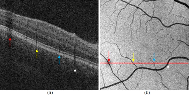
Vessel silhouettes appear as low-intensity regions disrupting the appearance of the ELM layer. (a) The arrows indicate vessel silhouettes formed by the vasculature of the retina. (b) The red line indicates the location of the slice shown in (a) on the en face projection image of the retina. Note the correspondence of the locations where vessels cross the slice and the location of the vessel silhouettes in the slice itself depicted by colored arrows.

Data Analysis

The OCT volumes of normal subjects were down-sampled in the y direction (direction of B-scan lines) to match the voxel size (240 μm) in the volumes of the subjects with CSME. Mean and 95% confidence interval of the detected disruption region volume was compared between the normal, normal down-sampled, and CSME subjects. Student's paired t-test was used to assess statistical significance of the area differences of disrupted regions of the ELM for the two groups of subjects. Three different threshold values of T (T = 0.4, 0.5, and 0.6) were applied to compute the disruptions as percentage over the whole volume, which aims at showing the robustness of the proposed method irrespective of T.

Results

Figure 3 shows the ELM layer segmentation, disruption area detection results, and surface views of the disruption areas on normal and CSME subjects. Figure 4 shows another example of ELM disruption area detection results on a subject with CSME with thickness information. The detected disruption region volume comparison on normal, normal down-sampled, and CSME subjects at three different threshold values, 0.6, 0.5, and 0.4, is shown in Figure 5. The mean and 95% confidence interval of the detected disruption volumes for normal, normal down-sampled, and CSME subjects (T = 0.5) were mean_normal = 0.00087 mm³ and CI_normal = (0.00074, 0.00100), mean_normal-ds = 0.00076 and CI_normal-ds = (0.00063, 0.00089), and mean_CSME = 0.00461 mm³ and CI_CSME = (0.00347, 0.00576) mm³, respectively. The paired t-test demonstrated strong statistical significance of the volume differences between the ELM disruption areas detected for CSME subjects and normal controls (both full-resolution and down-sampled, P < 0.001), while the area differences between the full-resolution and down-sampled normal image subjects were not statistically significant.

Figure 3.  .

The illustrations for the ELM layer disruption detection. The first column shows the original OCT image; the second column shows the contrast-enhanced OCT image by normalization; the third column shows the ELM layer segmentation results (indicated by red line) and disruption area detection results (indicated by yellow); and the fourth column shows the surface view of disruption area (indicated by yellow). The top and bottom rows show the results for normal and CSME subjects, respectively.

Figure 4.  .

An example of ELM disruption area detection. (a) One slice of the original OCT image. (b) Total retinal thickness (from top of RNFL to bottom of RPE). (c) ELM surface shown in red; ELM disruption regions shown in yellow. (d) ELM surface on which the disruption regions are marked in black. The red arrow points to the slice corresponding to slice location depicted in (a, c).

Figure 5.  .

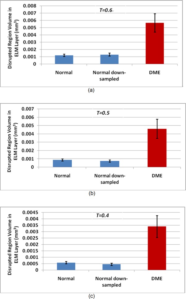
Detected disruption area volume comparison for normal, normal down-sampled, and CSME subjects. (a) T = 0.6; (b) T = 0.5; (c) T = 0.4. The plots show the averages and 95% confidence intervals.

Figure 6 shows the disruption voxel percentages in the ELM layer for normal, normal down-sampled, and CSME subjects at three different threshold values, T = 0.6, 0.5, and 0.4. Figures 7 through 9 show all examples of the ELM disrupted area detection results on the normal, normal down-sampled, and CSME subjects.

Figure 6.  .

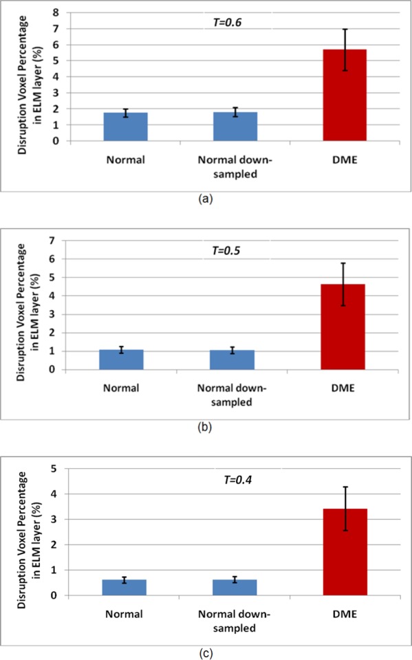
Disruption voxel percentage in ELM layer for normal, normal down-sampled, and CSME subjects. (a) T = 0.6; (b) T = 0.5; (c) T = 0.4. The plot shows the average and 95% confidence interval.

Figure 7.  .

ELM disrupted area detection results (indicated by yellow spots) on all 16 normal subjects in full-resolution Cirrus image data. Numerous pinpoint areas of 50 to 100 μm² ELM disruption exist, but no larger disruption areas were found.

Figure 8.  .

ELM disrupted area detection results (indicated by yellow spots) on all 16 normal controls (compare with full-resolution images shown in Fig. 7).

Discussion

We have developed and evaluated an automated method to quantify the 3-D integrity of the ELM in patients with CSME and in normal subjects. The results of this preliminary study show that in patients with CSME, large areas of disrupted ELM exist (Fig. 9), while in normal subjects the ELM is mostly continuous, and large disrupted areas do not exist. An unexpected finding was, however, that numerous small pinpoint areas of 50 to 100 μm² ELM disruption were detected in normal subjects. The impact of this finding is not clear at this moment.

Figure 9.  .

ELM disrupted area detection (in yellow) on all CSME subjects. Large areas of disrupted ELM are visible.

The classification of the ELM disruption area is based on texture and morphologic features. In this study, a threshold value of T was used for the disruption area classification. Three different threshold values of T were applied to compute the disruption volume as the percentages over the whole volume. Figure 7 demonstrates that the differences between disruption area sizes obtained from the normal and CSME subjects are very consistent regardless of the value of T. This observation demonstrates that the proposed method is robust with respect to the chosen values of T.

Because the resolution of normal data in the y direction is much higher than that of the CSME subjects, we have downsampled the normal OCT scans in the y direction to produce the same resolution (240 μm) as was achieved by clinical scanning in the CSME subjects. The experimental results in Figures 6 and 7 show that the disruption detection results are consistent for the normal and normal down-sampled subjects.

There are several shortcomings in this study. The study did not address the clinically more important question whether the ELM quantitative measures developed here correlate with visual acuity and visual outcome. The goal of this study was to demonstrate the development of this new quantitative technique, but a much larger study is needed to determine the association, if any, of these measures to visual acuity and visual outcome of CSME. First, the number of subjects was too small to allow determination of the performance of the proposed method. Second, there is no ground truth for the estimation of ELM disruption area, so the correlation analysis between the proposed method and the expert cannot be performed.

To our knowledge, this is the first method reported in the archival literature for automated and quantitative detection of ELM disruption areas in retinal OCT images. If our preliminary results can be confirmed in a larger study, algorithms to automatically estimate the ELM disruption area from SD-OCT have the potential to improve the management of patients with CSME.

In summary, in this preliminary study, we have developed a method for automated estimation of ELM disruption areas. The results showed that the detected ELM layer disruption is significantly larger in subjects with CSME than in normal subjects (P < 0.001). We have started determining the relationship of ELM disruption measures to visual acuity in patients with CSME.

References

- 1.Bhagat N, Grigorian RA, Tutela A, Zarbin MA. Diabetic macular edema: pathogenesis and treatment. Surv Ophthalmol. 2009;54:1–32 [DOI] [PubMed] [Google Scholar]
- 2.Ciulla TA, Amador AG, Zinman B. Diabetic retinopathy and diabetic macular edema: pathophysiology, screening, and novel therapies. Diabetes Care. 2003;26:2653–2664 [DOI] [PubMed] [Google Scholar]
- 3.Goldin A, Beckman JA, Schmidt AM, Creager MA. Advanced glycation end products: sparking the development of diabetic vascular injury. Circulation. 2006;114:597–605 [DOI] [PubMed] [Google Scholar]
- 4.Hee MR, Puliafito CA, Duker JS, et al. Topography of diabetic macular edema with optical coherence tomography. Ophthalmology. 1998;105:360–370 [DOI] [PMC free article] [PubMed] [Google Scholar]
- 5.Ahmed N. Advanced glycation endproducts—role in pathology of diabetic complications. Diabetes Res Clin Pract. 2005;67:3–21 [DOI] [PubMed] [Google Scholar]
- 6.Abràmoff MD, Garvin MK, Sonka M. Retinal imaging and image analysis. IEEE Trans Med Imaging. 2010;3:169–208 [DOI] [PMC free article] [PubMed] [Google Scholar]
- 7.Soliman W, Sander B, Jørgensen TM. Enhanced optical coherence patterns of diabetic macular oedema and their correlation with the pathophysiology. Acta Ophthalmol Scand. 2007;85:613–617 [DOI] [PubMed] [Google Scholar]
- 8.Wakabayashi T, Fujiwara M, Sakaguchi H, Kusaka S, Oshima Y. Foveal microstructure and visual acuity in surgically closed macular holes: spectral-domain optical coherence tomographic analysis. Ophthalmology. 2010;117:1815–1824 [DOI] [PubMed] [Google Scholar]
- 9.Sakamoto A, Nishijima K, Kita M, Oh H, Tsujikawa A, Yoshimura N. Association between foveal photoreceptor status and visual acuity after resolution of diabetic macular edema by pars plana vitrectomy. Graefes Arch Clin Exp Ophthalmol. 2009;247:1325–1330 [DOI] [PubMed] [Google Scholar]
- 10.Costa RA, Calucci D, Skaf M, et al. Optical coherence tomography 3: automatic delineation of the outer neural retinal boundary and its influence on retinal thickness measurements. Invest Ophthalmol Vis Sci. 2004;45:2399–2406 [DOI] [PubMed] [Google Scholar]
- 11.Otani T, Yamaguchi Y, Kishi S. Correlation between visual acuity and foveal microstructural changes in diabetic macular edema. Retina. 2010;30:774–780 [DOI] [PubMed] [Google Scholar]
- 12.Leung CK, Lam S, Weinreb RN, et al. Retinal nerve fiber layer imaging with spectral-domain optical coherence tomography: analysis of the retinal nerve fiber layer map for glaucoma detection. Ophthalmology. 2010;117:1684–1691 [DOI] [PubMed] [Google Scholar]
- 13.Wakabayashi T, Oshima Y, Fujimoto H, et al. Foveal microstructure and visual acuity after retinal detachment repair: imaging analysis by Fourier-domain optical coherence tomography. Ophthalmology. 2009;116:519–528 [DOI] [PubMed] [Google Scholar]
- 14.Theodossiadis PG, Grigoropoulos VG, Theodossiadis GP. The significance of the external limiting membrane in the recovery of photoreceptor layer after successful macular hole closure: a study by spectral domain optical coherence tomography. Ophthalmologica. 2011;225:176–184 [DOI] [PubMed] [Google Scholar]
- 15.Fernández EJ, Povazay B, Hermann B, et al. Three-dimensional adaptive optics ultrahigh-resolution optical coherence tomography using a liquid crystal spatial light modulator. Vision Res. 2005;45:3432–3444 [DOI] [PubMed] [Google Scholar]
- 16.Schmitz-Valckenberg S, Fleckenstein M, Göbel AP, Hohman TC, Holz FG. Optical coherence tomography and autofluorescence findings in areas with geographic atrophy due to age-related macular degeneration. Invest Ophthalmol Vis. Sci. 2011;52:1–6 [DOI] [PubMed] [Google Scholar]
- 17.Cho M, Witmer MT, Favarone G, Chan RP, D'Amico DJ, Kiss S. Optical coherence tomography predicts visual outcome in macula-involving rhegmatogenous retinal detachment. Clin Ophthalmol. 2012;6:91–96 [DOI] [PMC free article] [PubMed] [Google Scholar]
- 18.Li K, Wu X, Chen DZ, Sonka M. Optimal surface segmentation in volumetric images--a graph-theoretic approach. IEEE Trans Pattern Anal Mach Intell. 2006;28:119–134 [DOI] [PMC free article] [PubMed] [Google Scholar]
- 19.Li K, Wu X, Chen DZ, Sonka M. Efficient optimal surface detection: theory, implementation and experimental validation. In: Proceedings SPIE International Symposium on Medical Imaging: Image Processing. 2004;620–627 [Google Scholar]
- 20.Garvin MK, Abràmoff MD, Wu X, Russell SR, Burns TL, Sonka M. Automated 3-D intraretinal layer segmentation of macular spectral-domain optical coherence tomography images. IEEE Trans Med Imaging. 2009;28:1436–1447 [DOI] [PMC free article] [PubMed] [Google Scholar]
- 21.Garvin MK, Abràmoff MD, Kardon R, Russell SR, Wu X, Sonka M. Intraretinal layer segmentation of macular optical coherence tomography images using optimal 3-D graph search. IEEE Trans Med Imaging. 2008;27:1495–1505 [DOI] [PMC free article] [PubMed] [Google Scholar]
- 22.Lee K, Niemeijer M, Garvin MK, Kwon YH, Sonka M, Abràmoff MD. Segmentation of the optic disc in 3-D OCT scans of the optic nerve head. IEEE Trans Med Imaging. 2010;29:159–168 [DOI] [PMC free article] [PubMed] [Google Scholar]
- 23.Niemeijer M, Garvin MK, van Ginneken B, Sonka M, Abràmoff MD. Vessel segmentation in 3D spectral OCT scans of the retina. Proc SPIE Medical Imaging. 2008;6914:69141R;doi:10.1117/12.772680 [Google Scholar]