

Abstract
The local field potential (LFP) and multiunit activity (MUA) are extracellularly recorded signals that describe local neuronal network dynamics. In our experiments, the LFP and MUA, recorded from the same electrode in macaque primary visual cortex V1 in response to drifting grating visual stimuli, were evaluated on coarse timescales (∼1–5 s) and fine timescales (<0.1 s). On coarse timescales, MUA and the LFP both produced sustained visual responses to optimal and non-optimal oriented visual stimuli. The sustainedness of the two signals across the population of recording sites was correlated (correlation coefficient, ∼0.4). At most recording sites, the MUA was at least as sustained as the LFP and significantly more sustained for optimal orientations. In previous literature, the blood oxygen level-dependent (BOLD) signal of functional magnetic resonance imaging studies was found to be more strongly correlated with the LFP than with the MUA as a result of the lack of sustained response in the MUA signal. Because we found that MUA was as sustained as the LFP, MUA may also be correlated with BOLD. On fine timescales, we computed the coherence between the LFP and MUA over the frequency range 10–150 Hz. The LFP and MUA were weakly but significantly coherent (∼0.14) in the gamma band (20–90 Hz). The amount of gamma-band coherence was correlated with the power in the gamma band of the LFP. The data were consistent with the proposal that the LFP and MUA are generated in a noisy, resonant cortical network.
Introduction
The local field potential (LFP) and multiunit activity (MUA) are extracellularly recorded signals from a local network of neurons. The LFP, the low-frequency (<500 Hz) content of the raw recording, is believed to be generated by membrane currents of the neurons in the local neighborhood of the recording electrode. MUA, the high-frequency (>1000 Hz) portion of the recording, represents the spiking of local neurons.
Previous work on the relationship between the LFP and MUA includes studies of the spatial extent of the LFP as a function of nearby spiking neurons (Gieselmann and Thiele, 2008; Katzner et al., 2009; Xing et al., 2009), information conveyed by the LFP and spike data (Belitski et al., 2008), the ability to infer spikes from LFP data (Rasch et al., 2008), and the ability to infer the LFP from spike data (Rasch et al., 2009). The exact relationship between the LFP and MUA is still unclear (Kruse and Eckhorn, 1996; Logothetis et al., 2001; Buzsáki, 2002).
In this study, we examined the dynamic responses of the LFP and MUA recorded from anesthetized macaque primary visual cortex (V1) during visual stimulation with drifting gratings at optimal and non-optimal orientations. The LFP power spectrum has a peak in the gamma band (20–90 Hz) during visual stimulation (Gray and Singer, 1989; Frien et al., 2000; Logothetis et al., 2001; Siegel and König, 2003; Henrie and Shapley, 2005), and the dependence of LFP gamma-band power on stimulus contrast resembles the contrast–response functions of single V1 neurons (Henrie and Shapley, 2005). Therefore, we analyzed the relationship between the time-dependent responses of the LFP gamma-band power and MUA.
The time course of responses of the LFP and MUA are important in the effort to relate hemodynamic responses, as measured by the blood oxygen level-dependent (BOLD) signal in functional magnetic resonance imaging (fMRI) studies, to neuronal activity. An important question raised by previous studies is, how similar are the dynamic responses of MUA and the LFP to maintained stimulation? Previously, from studies of the connection of the LFP and MUA to the BOLD signal in anesthetized (Logothetis et al., 2001) and awake macaque V1 (Goense and Logothetis, 2008), it was reported that the MUA signal was less sustained than the LFP signal. This finding was one of the major results from which it was concluded that the BOLD signal was not directly dependent on MUA and rather that the BOLD signal was primarily correlated with the LFP (Logothetis et al., 2001; Logothetis, 2002). To answer the question of how similar the dynamic responses of the MUA and LFP are, we analyzed responses from many V1 recording sites on coarse timescales (3–5 s). We used a “sustained index” (SI) (the ratio of sustained response to the peak response) to capture the global shape of the dynamics of MUA and LFP gamma power. As reported in Results, for optimally oriented visual stimuli, MUA was significantly more sustained than the LFP. For the population of all oriented stimuli, in a small majority of recording sites the MUA response was more sustained than the LFP gamma-band response, but the distributions were statistically indistinguishable. There was large variability in the relative size of the sustained component of the response, for both signals, and the sustained components of MUA and the LFP gamma band were correlated. Our findings of equally sustained LFP and MUA responses suggests that the neuronal sources of the BOLD signal should be reconsidered (Nir et al., 2007).
Because of the correlation of sustained components across the population, we also examined the dependence of the LFP and MUA on fine timescales (<0.1 s) using spectral coherence analysis (Mitra and Pesaran, 1999; Shumway and Stoffer, 2000; Pesaran et al., 2002). The LFP and MUA had a small but significant peak in coherence (∼0.14) centered in the gamma band. The value of peak coherence between MUA and the LFP depended on the amount of power in the LFP gamma band. The weakness of coherence between the two signals could be a result of nonlinear signal processing in the cortical network and/or could be a result of the contributions of non-overlapping neuronal populations to the LFP and MUA.
Materials and Methods
Surgery and preparation.
Acute experiments were performed on adult Old World monkeys (Macaca fascicularis). All surgical and experimental procedures were performed in accordance with the guidelines published in the National Institutes of Health Guide for the Care and Use of Laboratory Animals (publication number 86-23, revised 1987) and were approved by the University Animal Welfare Committee at New York University. Animals were tranquilized with acepromazine (50 μg/kg, i.m.) and anesthetized initially with ketamine (30 mg/kg, i.m.) and then with isoflurane (1.5–3.0% in air). After cannulation and tracheotomy, the animal was placed in a stereotaxic frame and maintained on opioid anesthetic (sufentanil citrate, 6–12 μg · kg−1 · h−1, i.v.) for craniotomy. A craniotomy (∼5 mm in diameter) was made in one hemisphere posterior to the lunate sulcus (∼15 mm anterior to the occipital ridge, ∼10–20 mm lateral from the midline). A small opening in the dura (∼3 × 3 mm2) was made to provide access for multiple electrodes. After surgery, the animal was anesthetized and paralyzed with a continuous infusion of sufentanil citrate (6–18 μg · kg−1 · h−1, i.v.) and vecuronium bromide (0.1 mg · kg−1 · h−1, iv). Vital signs, including heart rate, electroencephalogram, blood pressure, oxygen level in blood, and urine-specific gravity, were closely monitored throughout the experiment. Expired carbon dioxide was maintained close to 5%, and rectal temperature was kept at 37°C. A broad-spectrum antibiotic (Bicillin, 50,000 IU/kg, i.m.) and anti-inflammatory steroid (dexamethasone, 0.5 mg/kg, i.m.) were given on the first day and every other day during the experiment. The eyes were treated with 1% atropine sulfate solution to dilate the pupils and with a topical antibiotic (gentamicin sulfate, 3%) before being covered with gas-permeable contact lenses. Foveae were mapped onto a tangent screen using a reversing ophthalmoscope. Proper refraction was achieved by placing corrective lenses in front of the eyes on custom-designed lens holders.
Electrophysiological recordings and data acquisition.
The Thomas seven-electrode system was used to record simultaneously from multiple cortical cells in V1. The seven electrodes were arranged in a straight line with each electrode separated from its neighbor by 300 μm. Each electrode consisted of a platinum/tungsten core (∼25 μm in diameter and ∼1 μm at the tip) covered with an outer quartz–glass shank (∼80 μm in diameter) and had an impedance value of 0.7–4 MΩ. Electrical signals from the seven electrodes were amplified, digitized, and filtered (0.3–10 kHz) with RA16SD preamplifiers in a Tucker-Davis Technologies System 3 configured for multichannel recording. The Tucker-Davis system was interfaced to a Dell personal computer that ran a multichannel version of the OPEQ program (written by Dr. J. A. Henrie, in our laboratory) to acquire both spike and local field potential data. Visual stimuli were generated with the custom OPEQ program, running in Linux on a Dell personal computer with a graphics card with Open GL optimization. Data collection was synchronized with the screen refresh to a precision of better than 0.01 ms. Stimuli were displayed on an IIyama HM 204DTA flat color graphic display (size, 40.38 × 30.22 cm2; pixels, 2048 × 1536; frame rate, 100 Hz; mean luminance, 53 cd/m2). The screen viewing distance was 115 cm so that the full cathode ray tube screen subtended 20° × 15° visual angle, approximately.
Visual stimulation.
Once all seven electrodes were located in the same layer, an experiment was run with drifting sinusoidal gratings (at high contrast, spatial frequency at 2 cycle/°, temporal frequency at 4 Hz) within a circular patch of diameter 3° visual angle, covering the visual field locations of all recording sites. Mean luminances within the stimulus patch and on the rest of the blank screen were the same. The stimulus drifted in different directions between 0° and 360°, in 20° steps in a pseudorandom order. The stimulus in each condition was presented for 2 or 4 s, repeated between 25 and 50 times depending on the experiment.
Continuous Gabor transform.
To study the dynamic relationship of the LFP and MUA on coarse timescales, we used a time–frequency analysis with the continuous Gabor transform (CGT) (cf. Burns et al., 2010). The CGT is a short time, or windowed, Fourier transform (also called a complex spectrogram) that retains the time dependence of the spectrum that is lost in the Fourier transform (Mallat, 1999, p 69). The continuous transform differs from the discrete version in that the signal is oversampled in time and frequency so that neighboring points are not independent. The Gabor filter ψ(t, ω0) used here is a one-dimensional plane wave with frequency f0 (in hertz; ω0 = 2πf0) windowed with a Gaussian:
 |
The CGT of a signal h(t) is found by convolving the Gabor filter function with h(t) and results in a complex time series H(t0)exp{iϕ(t0)} that represents the amplitude and phase of the signal at the frequency of the Gabor filter, ω0:
 |
In time–frequency analyses, the uncertainty principle limits the resolution that can be resolved in the temporal and spectral domains. This limitation is expressed by the parameter σ in Equation 1. A balance between the time and frequency resolutions must be found that captures the characteristics of interest for the time series being studied. If the characteristic width of the Gabor filter is considered to be two e-folding lengths (the distance at which the Gaussian envelope is e−2 less than its peak value), the uncertainty condition for the CGT is as follows:
 |
where δt is the time resolution, and δw is the frequency resolution.
R-spectrum. The R-spectrum, as used here, is defined to be the visually stimulated power spectrum divided by the spontaneous (unstimulated) power spectrum at each frequency:
 |
The R-spectrum is useful for expressing the stimulated power spectrum in normalized dimensionless units that can be compared across experiments. When R(f) > 1, the stimulated spectrum has elevated power compared with the spontaneous activity.
Line noise filtering.
In the data collected, there was a strong line noise signal at 60 Hz. Over the length of the recordings, the amplitude of the line noise was constant but its phase drifted. To filter out the line noise signal from the LFP recording, the amplitude of the 60 Hz signal line noise was estimated from the spectrum of the raw signal. This estimate was found by taking the Fourier transform of the entire record and interpolating the amplitude at 60 Hz from its neighboring values as an estimate of the 60 Hz component of the LFP signal. The amplitude of the line noise was assumed to be the difference between the interpolated amplitude and measured amplitude. To determine the phase of the line noise during each 2–4 s experiment, a sine wave with the computed line noise amplitude was regressed on to the subsamples of the record used in the analysis. This method was used to removed the line noise at 60 Hz effectively and at higher harmonics (120 and 180 Hz).
Results
The data analyzed here were from 51 extracellular recordings of macaque V1 from two monkeys lightly anesthetized with the opioid sufentanil. Of the 51 experiments, 43 were selected for analysis on the basis of two criteria: (1) they exhibited a visual response in excess of 3 SDs above the spontaneous activity within 0.25 s of the stimulus onset, and (2) the MUA and LFP signals did not have any instrumental artifacts (in 7 of 51, sites the recordings had dropouts in the recorded signal resulting from problems with equipment). There were 25–50 repeated trials for each of the 43 experiments, with each trial consisting of a baseline blank (no stimulus) for 1 s and high-contrast, large, drifting grating stimulus oriented at angles that gave the optimal maximum response and non-optimal angles for 2 or 4 s depending on the experiment.
Visual responses of MUA and the LFP
A Student's t test was used to assess whether the mean spontaneous activity was significantly different from the mean sustained response for each signal. The mean spontaneous activity was taken from the first 0.5 s of data before the stimulus was presented, and the mean sustained response was taken from the last second of the stimulated period excluding 0.25 s at the end of the stimulus to avoid including offset effects. For both the MUA and LFP, the mean spontaneous and mean sustained responses were found to be drawn from different distributions at the 95% confidence limit. All trials examined here also had significantly elevated gamma-band spectral power in the LFP during visual stimulation. The population average R-spectrum (see Materials and Methods) is plotted in Figure 1A. On average, the population had strongly peaked, elevated power centered at 44 Hz. A histogram of the peak R-spectrum values across the population of sites is plotted in Figure 1B. The histogram shows that all sites had a peak R-spectrum power >1 in the gamma band, indicating that there was elevated gamma power during visual stimulation. The hatched bin in the histogram in Figure 1B contains all sites that had peak R-spectrum power in the gamma band that was >9.
Figure 1.
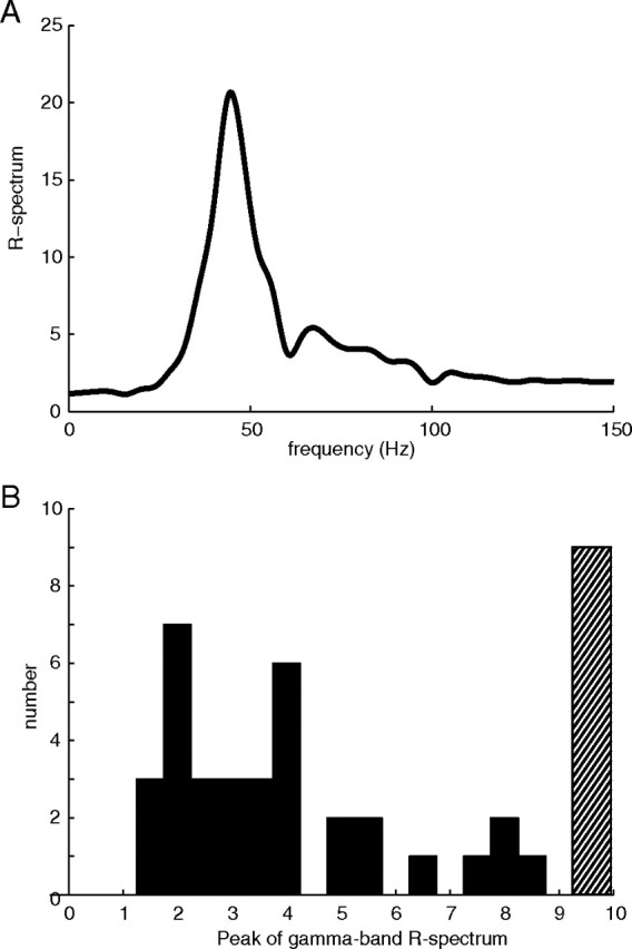
A, Population average R-spectrum (stimulated power spectrum divided by spontaneous power spectrum; see Materials and Methods); the power spectrum of the response to visual stimulation is dominated by a peak in the gamma band centered around 40 Hz. B, Histogram of population maximum gamma-band (20–90 Hz) R-spectrum (>9 placed in hatched bin above 9). All sites had maximum R-spectrum values in the gamma band greater than 1, indicating a response to the stimulus.
Coarse timescale dynamics
On coarse timescales (1–5 s), we studied the sustained properties of the LFP and the MUA relative to their peak responses during drifting grating visual stimulation. The gamma band of the LFP is the frequency range most strongly driven by a visual stimulus (Gray and Singer, 1989; Frien et al., 2000; Logothetis et al., 2001; Siegel and König, 2003; Henrie and Shapley, 2005), as is evident for our data in Figure 1A. Therefore, we compared the gamma-band power as a function of time with the MUA.
The time-dependent gamma-band power signal was derived from the extracellular raw field potential (RFP) recording shown schematically in Figure 2. The LFP was formed by low-pass filtering the RFP at 500 Hz, and the LFP gamma-band power signal was generated by computing the CGT (see Materials and Methods) with a window width of 50 ms for the length of the trial (2 or 4 s) and summing the Gabor amplitude spectrum over the frequencies 20–60 Hz. The LFP gamma-band power signal was computed for each trial, and the average LFP gamma-band power for each site was found by averaging the LFP gamma-band power from all trials at that site.
Figure 2.

Coarse timescale signal generation. MUA: Each trial is convolved with a Gaussian kernel whose width matches that used for the LFP spectrogram, and the site average is found by averaging all Gaussian kernel smoothed trial MUA recordings, RFP: For each trial, the MUA is formed by thresholding the RFP at 3 SDs and recording binary spikes in a separate file when large-amplitude transients occur, and the LFP is formed by low-pass filtering the RFP at 500 Hz. LFP: The gamma-band power time series for each trial is formed by averaging the spectrogram of the LFP over the frequencies between 20 and 60 Hz; the site average gamma-band power time series is found by averaging over all gamma-band power time series from all trials at that site.
The computation of the MUA from the RFP is also shown in Figure 2. For each trial, the MUA signal was computed by thresholding the RFP at 3 SDs. Each time the RFP exceeded the 3 SD threshold, a one was recorded in a separate file that otherwise contained zeroes in which the amplitude of the RFP was below threshold. The experimental average of the MUA signal was computed by averaging over all trial MUAs and was smoothed in time by convolving the average MUA with a temporal Gaussian the width of which matched that used in the Gabor transform of the LFP so that the MUA could be compared with the LFP gamma-band power signal.
Comparisons between MUA and LFP responses were performed at the grating orientation that gave the largest MUA response (optimal orientation stimuli) and across multiple grating orientations (all oriented stimuli). The first 2 s of the population mean MUA and LFP gamma-band power responses to optimal orientation visual stimuli (blue) and all oriented visual stimuli (red) are plotted in Figure 3. The mean raw responses with the baseline removed from each site are plotted in Figure 3, A and B (the units in these two plots are not informative but are presented to show the raw response compared with the normalized response). The responses with the baseline from each site removed and normalized by the peak response at each site are plotted in Figure 3, C and D. The response in both the raw and normalized time courses show a slight decrease in the MUA between optimal and all orientations of the stimuli and little change in the LFP, indicating that the MUA was more narrowly tuned than the LFP to the orientation angle of the stimuli. The coarse timescale similarity between the raw and normalized responses also demonstrates that our method of normalization does not strongly affect the nature of the response of the two signals.
Figure 3.

The population average MUA and LFP gamma-band power responses to optimal orientation stimuli (blue) and all oriented stimuli (red). A, Population average raw MUA responses. B, Population average raw LFP gamma-band power responses. C, Population average normalized MUA responses. D, Population averaged normalized LFP gamma-band power responses. The MUA is more narrowly tuned to angle of the drifting grating visual stimuli than the LFP gamma-band power, and the normalization of the signals does not qualitatively change the coarse timescale characteristics of the two signals.
Sustained index
The sustained nature of the responses of the LFP and MUA to visual stimulation was examined to determine whether or not the two signals show prolonged activity to visual stimulation. The features that were used to compare the LFP and MUA on coarse timescales were as follows: (1) the height of the peak response of the signal during stimulation (Peak), (2) the average elevation of the sustained response measured during the last second of the visual stimulus with the last 0.25 s excluded (μS), and (3) the mean spontaneous activity measured from the half second before stimulus onset (μB). These quantities are shown in Figure 4 for responses from one site. The SI, defined as
 |
was used to measure the size of the sustained response relative to the mean spontaneous activity.
Figure 4.
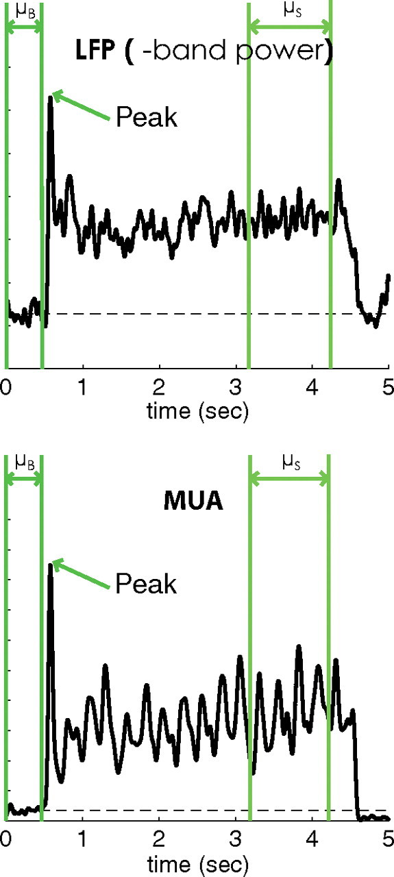
Trial average MUA and LFP gamma power from one site. Plotted in green are the features of the LFP and MUA used in the SI of the two signals. SI = (μS − μB)/(peak − μB).
Larger values of the sustained index indicated a larger sustained response during stimulation.
Coarse timescale results
The coarse timescale results revealed that, on average, MUA was more sustained than the LFP, and there was large variability from site to site across the population. In the data considered here for optimally oriented stimuli, a majority of experiments (29 of 43 sites) had a more sustained MUA response. Figure 5A is a scatter plot of the SIs for the 43 experiments examined. For each data point, both the LFP gamma-band power and smoothed MUA were averaged over all trials at that site to generate the site mean time series from which the indices were calculated according to Equation 5. Points that lie above the unity line in Figure 5A (solid blue line) indicate that the response of the MUA was more sustained than the LFP. In general, sites that produced a more sustained LFP response tended to produce more sustained MUA responses with a correlation coefficient of 0.37. The scatter plot has a linear regression (dashed blue line) with a slope of 0.46 (p = 0.014). Plotted in Figure 5B are the histograms of the sustained indices for the MUA and LFP along with their mean values and SDs. More sites had more sustained MUA responses, and the population mean MUA SI was larger than the population mean LFP SI (mean ± SD MUA SI of 0.46 ± 0.17 and mean ± SD LFP SI of 0.37 ± 0.14). A Student's t test of the distribution of SI values from the 43 sites showed that the MUA and LFP SI distributions had statistically significant different means, with p = 0.015.
Figure 5.
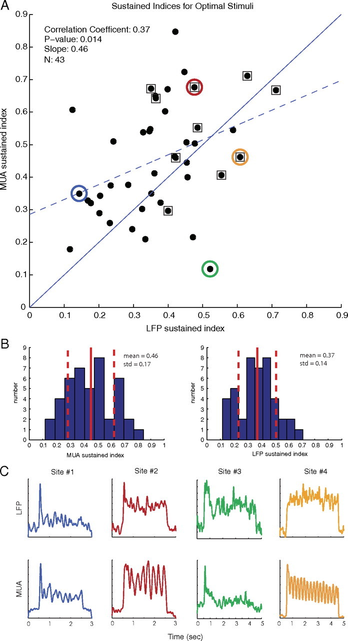
A, Scatter plot of sustained indices in response to optimally oriented stimuli with linear regression (dashed blue line) and reference unity line (solid blue line). Sites with MUAs that track the phase of the visual stimulus are surrounded by a square. There was a large amount of variability in the response of the LFP and MUA, but a majority of points lie above the unity line, indicating that more sites had MUAs that were more sustained than LFPs. B, Histograms of the population MUA and LFP sustained indices for optimal stimuli with mean and SD. On average, the MUA was more sustained then the LFP for stimuli at the optimal orientation. C, LFP and MUA responses of four example cells to optimal stimuli; the indices of these responses are color coded in the scatter plot. A wide variety of responses are seen for both the MUA and LFP at individual sites.
Examples of MUA and LFP recordings from four individual sites are plotted in Figure 5C to demonstrate the range of responses seen in the data. The time courses of the example cells are color coded with their corresponding points in the sustained indices scatter plot in Figure 5A. Sites 1 and 2 are examples of typical behavior seen in the data with an MUA response that was more sustained than the LFP. At Site 4, although the LFP was more sustained, there was still a sustained response in the MUA as well. Responses at Site 3 resembled the findings reported by Logothetis et al. (2001) and Goense and Logothetis (2008) in which the LFP was sustained and the MUA returned to baseline shortly after the stimulus onset. Another feature of the data is that, at Sites 2 and 4, the MUA tracked the 4 Hz oscillation of the drifting grating visual stimulus although the LFP did not. At 10 of the 43 sites examined, MUA signals tracked the temporal phase of the drifting grating stimulus at a level of 2 SD above the mean sustained response but, in our dataset, there were no sites with LFPs that had this property. Sites with MUAs that tracked the phase of the stimulus are denoted in Figure 5A by points surrounded by a square.
We also compared the SIs of the MUA and LFP using the orientation of the stimuli that gave the largest response in the gamma band of the LFP rather than the largest MUA response. The data were collected at the optimal orientation for the MUA response and non-optimal MUA orientation at ∼30–40° (and some sites also 90°) away from optimal MUA orientation. Of the 43 sites shown in Figure 5, 27 sites had recordings at one to two non-optimal stimulus orientations. Data were not specifically collected for the orientation that gave the optimal LFP response, but, from the orientations that were recorded, we selected that orientation that gave the largest increase in power in the gamma band of the LFP. We found that only 7 of the 43 sites studied had an LFP optimal orientation that was different from the MUA optimal orientation. An analysis of the LFP optimal orientation data, plotted in Figure 6, showed no qualitative difference compared with using the MUA optimal orientation. Using the LFP optimal orientation, a majority of sites still had a more sustained MUA than LFP (27 of 43), the mean of the MUA sustained indices was 0.46, and the mean of the LFP sustained indices was 0.39. A scatter plot of the population SI values and histograms of the MUA and LFP SI values for LFP optimal oriented stimuli are shown in Figure 6, A and B, respectively.
Figure 6.
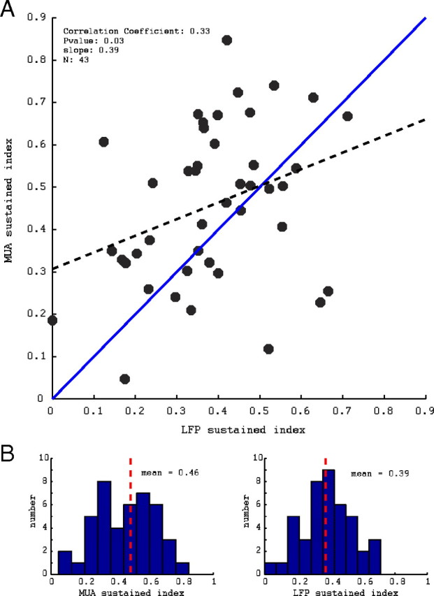
A, Scatter plot of the sustained indices of the MUA and LFP in response to stimuli oriented to give the maximum gamma-band LFP response with linear regression (dashed black line) and reference unity line (solid blue line). B, Histograms of the population MUA and LFP sustained indices for optimal LFP oriented stimuli with mean. The relationship between the sustained indices of the MUA and LFP and the population means are not qualitatively changed when optimal LFP stimuli are used rather than optimal MUA stimuli as in Figure 5.
To compare the results found here with previous studies that used more complex visual stimuli, which contained features at many orientations (such as the rotating checkerboard stimulus used by Logothetis et al., 2001; Goense and Logothetis, 2008), we also analyzed the sustained responses of the MUA and LFP at non-optimal stimulus orientations rather than only the responses to optimal orientations shown in Figures 5 and 6. The MUA and LFP SIs of the population of all optimal and non-optimal orientations (74 experiments from 43 sites) are plotted in Figure 7A. When the MUA and LFP at all oriented stimuli are compared, a majority of sites had more sustained MUA responses (42 of 74 sites), and the correlation coefficient (0.37) and slope of the regression (0.46, p = 0.002) were similar to that seen in the analysis of responses to the optimal orientation only. Plotted in Figure 7B are the histograms of the SI values for the MUA and LFP. The mean ± SD of the MUA SIs was slightly reduced (compared with the optimal-only data) to 0.44 ± 0.17, and the mean ± SD of LFP SIs was slightly larger at 0.41 ± 0.15. A Student's t test between the distributions of MUA and LFP SIs for all orientations reveals that the distributions were statistically indistinguishable, with p = 0.26. We have also analyzed only the non-optimal orientations (data not shown); these had qualitatively similar properties to the population of all orientations plotted in Figure 7. The mean ± SD non-optimal MUA SI was 0.41 ± 0.17, and the mean ± SD SI of the non-optimal LFP was 0.45 ± 0.16, with a correlation coefficient between MUA and LFP of 0.44. A Student's t test of the distribution of SI values for the MUA and LFP showed that the two distributions of sustained indices at the non-optimal sites were statistically indistinguishable, with p = 0.30.
Figure 7.
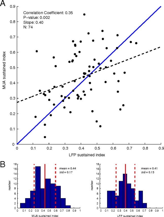
A, Scatter plot of sustained indices in response to all oriented stimuli with linear regression (dashed blue line) and reference unity line (solid blue line). B, Histograms of the population MUA and LFP sustained indices for all oriented stimuli with mean and SD. When all orientations are included, the mean MUA and LFP response are nearly equal.
At some sites, there was a spike in the power spectrum at 100 Hz, corresponding to the refresh rate of the monitor used to present the visual stimuli. To measure the strength of the 100 Hz signal present at each site, the 100 Hz power index was defined to be the value of the power spectrum at 100 Hz divided by the mean of the power spectrum over ranges of 95–98 and 102–105 Hz. The 100 Hz power index is dimensionless and, over the population of 43 sites, varied from 0.8 to 7.7. To determine whether the sustained properties of the MUA and LFP gamma-band power signals were affected by the flickering of the monitor, the sustained indices of the MUA and LFP at optimal orientation were compared with the 100 Hz power index in Figure 8. For both the MUA (Fig. 8A) and LFP (Fig. 8B), there was no structure to the scatter plots. The correlation coefficients of the MUA SI and LFP SI with the 100 Hz power index were −0.038 and −0.26, respectively, indicating that there was no correlation between the sustained properties of the MUA and LFP and entrainment to the monitor refresh rate.
Figure 8.

A, Scatter plot of the sustained indices of the MUA at the MUA optimal response orientations compared with the 100 Hz power index. B, Scatter plot of the sustained indices of the LFP at the MUA optimal response orientations compared with the 100 Hz power index.
Fine timescale dynamics
Another way to probe the relation between MUA and the LFP was to study their correlation on fine timescales (<100 ms) by computing their coherence (Mitra and Pesaran, 1999; Shumway and Stoffer, 2000; Pesaran et al., 2002) during the sustained period of their response to visual stimulation. The coherence, a measure of the correlation between two signals as a function of frequency, is the Fourier transform of the normalized cross-covariance between two signals (Mitra and Pesaran, 1999; Shumway and Stoffer, 2000; Pesaran et al., 2002). The coherence between the MUA and LFP is defined as follows:
 |
where Fa(f) is the complex-valued Fourier coefficient of signal a(t) at frequency f, and Sa(f) is the power spectrum of signal a(t). To compute the coherence, the LFP was formed by simply low-pass filtering the RFP at 500 Hz, and MUA was the same signal used in the coarse timescale analysis but without the smoothing by a Gaussian window. The coherence between the LFP and MUA was found by computing the product of the Fourier transforms of each signal (numerator of Eq. 6) and power of each signal (denominator of Eq. 6) during the period of stimulation averaged over 500 ms overlapping segments smoothed with a Hamming window to reduce spectral artifacts. The initial 0.25 s and the last 0.25 s of visual stimulation were excluded to remove onset and offset transients.
To determine the portion of the coherence that was extrinsically driven by the visual stimulus and was common to all trials, a shift-predictor coherence was computed. The shift predictor was generated by computing the coherence between the LFP from one experimental trial and MUA from the same site but from a different trial separated in time. Any coherence found between these signals was assumed to be caused by direct drive of the visual stimulus and not a result of the internal V1 network dynamics. Here we picked a shift of 10–20 trials to ensure that the shifted trials were well separated in time. The mean of the shift-predictor coherence was bootstrapped to generate a 95th percentile that was used to test the statistical significance of the nonshifted coherence. The bootstrapped 95th percentile was found by generating an ensemble of site mean shift-predictor coherences. Each bootstrapped site mean shift-predictor coherence in the ensemble was formed by taking the mean of a randomly selected with replacement subpopulation, whose number matched the number of trials at that site, of all the shift-predictor coherences at that site. An ensemble of 1000 bootstrapped mean shifted coherences was generated and sorted at each frequency from which the 95th percentile was determined.
Fine timescale results
The data indicate there was on average weak coherence between the LFP and MUA signals, and coherence was concentrated in the gamma band. The population average coherence between the LFP and the MUA is plotted in Figure 9A along with the deterministic (stimulus-driven) component of coherence measured with the population average shift predictor. The 95th percentile of the bootstrapped population average shift-predictor coherence is plotted in blue along the top of the yellow-shaded region, and the population mean shift-predictor coherence is plotted in green at the bottom of the shaded region. The regions in which the coherence exceeded the 95th percentile of the shift predictor (rises above the shaded region) were statistically significant. In Figure 9A, the average coherence is strongest and significant in the gamma band with a peak value of 0.14 at 42 Hz and a second smaller peak at 82 Hz near the second harmonic of the main peak. The peak at 100 Hz is attributable to the entrainment of the monkey's visual system to the refresh rate of the monitor used to present the visual stimulus, and the smaller peaks at 90 and 110 Hz are probably noise.
Figure 9.
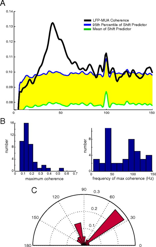
A, Coherence between the LFP and MUA with shift-predictor coherence: LFP–MUA coherence (black), mean shift-predictor coherence (green), and 95th percentile of the shift predictor coherence (blue). The regions of statistically significant coherence occur when the coherence exceeds the 95th percentile of the shift-predictor coherence. B, Histograms of the maximum coherence of each experiment (left) and of the frequency at which the maximum coherence occurs (right) C, Polar plot of the average maximum coherence as a function of frequency (angle, frequency; radius, average maximum coherence). The largest maximum coherences are associated with gamma-band frequencies (30–50 Hz), with weaker maximum coherence at 100 Hz (monitor refresh rate).
In Figure 9B, the histogram of the maximum coherence of each experiment is plotted on the left, and the histogram of the frequency at which the maximum coherence occurs is plotted on the right. The mode of the maximum coherence histogram is ∼0.15. There were eight experiments that had large coherences in the range 0.2 < coherence < 0.6. The histogram of the frequency of the peak coherence shows that most peak coherences occur either in the gamma band near 40 Hz or at the 100 Hz monitor refresh rate. A polar plot of the average peak coherence as a function of frequency (Fig. 9C) shows that the largest coherences occur in the gamma band with the secondary peak at 100 Hz, the monitor refresh rate.
Gamma-band coherence and LFP gamma-band power
The LFP exhibited elevated gamma-band power during visual stimulation and the MUA and LFP were weakly coherent in the gamma band. In this section, we address the relationship between the LFP gamma-band power and the strength of the gamma-band MUA–LFP coherence. To quantify the magnitude of the LFP gamma-band power, the R-spectrum (see Materials and Methods) was used to express the stimulated LFP power spectrum in terms of the spontaneous LFP power. The peak of the LFP gamma-band power under visual stimulation was characterized using the gamma-power index (GPI), defined as follows:
 |
In Figure 10A, a scatter plot of the maximum coherence between the LFP and MUA in the gamma band for each experiment is plotted against the GPI. The linear regression (p < 0.005) is also plotted. The correlation coefficient between the maximum gamma-band coherence and the GPI is 0.42. If we interpret as usual the LFP as the average membrane current in a local neighborhood, then the increased GPI is a an index of the degree of synchronization of nearby membrane currents around a gamma-band peak (Zeitler et al., 2006). The increased coherence of MUA and the LFP with increasing GPI therefore seems very natural because the spiking neurons that contribute to the MUA also are likely to be part of the population of cells that contribute to the LFP (Xing et al., 2009). Example sites are plotted in Figure 10B and are color coded with their corresponding points in the scatter plot (95th percentile of the shift predictor for each site plotted in black). Sites 3 and 6 lie near the regression line; they exhibited gamma-band coherence peaks that were positively correlated with GPI, as is characteristic of the population. Site 1 had a large gamma-band coherence and large GPI. The other three sites are outliers. Sites 2 and 5 had large gamma-band coherence peaks but with a smaller GPI, whereas Site 4 had no gamma-band coherence peak but did have a large GPI.
Figure 10.
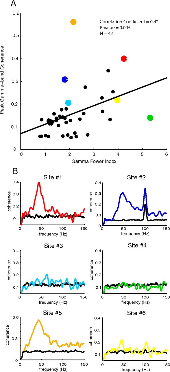
A, A scatter plot of the GPI and the maximum gamma-band coherence; the coherence in the gamma band increases as the gamma-band power increases. B, Example sites color coded with their corresponding points in the scatter plot (95th percentile of the shift predictor for each site is plotted in black).
Discussion
In this study, the MUA and LFP had similar population average sustained responses to visual stimulation, but, across the population, there was large variability in the temporal persistence of responses from site to site. For optimally oriented stimuli, the MUA had a more sustained response in a majority of experiments (29 of 43 sites), and, on average, the MUA had a significantly larger sustained index value. Furthermore, although there was a large amount of variation in the sustained index across the population of cortical recording sites, there was a substantial correlation, ∼0.4, between the amount of sustained response in the LFP and MUA.
Sustainedness of MUA and the LFP
The time courses of the responses of MUA and the LFP have implications for relating cortical activity to the BOLD signals measured with fMRI, a topic that has inspired much recent research (Logothetis et al., 2001; Almeida et al., 2002; Masino 2003; Kim et al., 2004; Sheth et al., 2004; Kayser et al., 2004; Tolias et al., 2005; Shmuel et al., 2006; Martin et al., 2006; Viswanathan and Freeman, 2007; Vakorin et al., 2007; Goense and Logothetis, 2008; Huttunen et al., 2008; Angenstein et al., 2009; Martuzzi et al., 2009). Both Logothetis et al. (2001) and Goense and Logothetis (2008) explicitly state that the BOLD signal was found to be more strongly correlated with the LFP than with the MUA as a result of the lack of sustained response in the MUA signal. Our results are at odds with the conclusions of Logothetis et al. (2001) and Goense and Logothetis (2008) in that we find that the MUA, for optimal stimuli, is often significantly more sustained than the LFP and is at least as sustained as the LFP for non-optimal stimuli.
There were a number of differences between the work by Logothetis et al. (2001) and Goense and Logothetis (2008) (hereafter referred to as L2001 and GL2008) and our study reported here. In the studies of L2001 and GL2008, a bandpass filtering technique was used to generate the different signals. We reanalyzed our data using the bandpass filtering method described by GL2008 and found that using their data analysis method did not qualitatively change our stated results but did generate more temporal smoothing of the signals compared with our analysis. Another difference is that L2001 and GL2008 used a rotating checkerboard pattern as a visual stimulus rather than the drifting grating pattern used here. To recreate the possible response to a rotating checkerboard stimulus from our data, we analyzed the sustained indices of the MUA and LFP at non-optimal as well as optimal orientations. For all orientations, we found that a majority of sites still had a slightly more sustained MUA, but the mean SIs were statistically indistinguishable. The number of recording sites examined also differed between studies. In the study by L2001, data were recorded from 29 sites and that by GL2008 from 14 sites, both of which are less than the 43 sites studied here. Based on the large variability in MUA and LFP responses seen our data (Fig. 4), it is possible that the results of L2001 and GL2008 were affected by their smaller sample size. It is difficult to determine population statistics by both L2001 and GL2008 because all plots are of individual sites or population mean responses. Furthermore, despite their reports of finding transient responses in the MUA in a minority of sites examined (⅕ of 14 sites in the study by GL2008 and ¼ of 29 sites in that by L2001), both studies concluded that the MUA was more transient than the LFP, a conclusion that we think required stronger support than the data offered.
Although we found a large variation in the sustained properties of the LFP and MUA from site to site, the population average sustained indices of the MUA is greater than the LFP (Fig. 4B). This implies that the sustained signal that the BOLD records, which is averaged over a cortical volume that is large compared with one of our recording sites, would likely receive a larger contribution from the sustained response of the MUA than the LFP. Furthermore, using a t test, we found that, for all experiments, the mean sustained activity was found to be significantly different from the spontaneous activity at the 95% confidence limit for both MUA and LFP signals. The fact that the MUA is as sustained as the LFP is significant because it suggests that, based on the arguments of L2001 and GL2008, the BOLD signal is as likely to be correlated with MUA as with the LFP. For these reasons, we conclude that MUA, the spiking activity of the population of neurons in the network, may also be correlated with the BOLD signal, and the possibility that the BOLD signal contains information about the spiking output of local networks of neurons should be reconsidered (cf. Nir et al., 2007).
Implications of coherence analysis
It has been proposed that the LFP represents the input to a neuronal network and MUA the spiking output (Logothetis, 2002). According to this hypothesis, the LFP supplies the external drive and the MUA is a response to that drive through the filtering of the thresholds of the cells and spike-firing mechanisms (Buzsáki, 2002; Logothetis and Wandell, 2004). However, although we found that the LFP and MUA were somewhat correlated on coarse timescales, on finer timescales these signals were only very weakly coherent, with a small but significant peak in coherence located in the gamma band. Despite the fact that the LFP and MUA are recorded from the same electrode and that the spikes in the MUA contain spectral components at low frequencies, there is only weak coherence between the LFP and MUA. This weak coherence indicates there is little leakage of the spiking signal down into the lower frequencies of the LFP. The coherence results suggest that the relation between MUA and the LFP may be more complex than simply the input to and output from the locally recorded network.
We also found there was a significant correlation between the amount of power in the gamma band of the LFP and the amount of gamma-band coherence present between the LFP and the MUA. This latter result fits with a picture of the local field potential as the average of local membrane currents reflecting the summed activity of hundreds of neurons, whereas MUA may be averaging the spiking of on the order of 10 neurons (Zeitler et al., 2006).
Relation between MUA and the LFP
Suppose V1 is a highly recurrent network that generates gamma-band activity dependent on the strength of stimulation (Henrie and Shapley, 2005; Kang et al., 2010) and other stimulus variables. The similarities between the population averaged sustainedness of MUA and the LFP may reflect the fact that the dynamics of both signals are strongly influenced by recurrent cortical interactions. The correlation of sustained indices we found may be accounted for by the fact that MUA and the LFP are different samples from a similar cortical population. Different sampling of the population statistics of a recurrent network by MUA and the LFP also could explain the weak gamma-band coherence between MUA and the LFP (Zeitler et al., 2006) and the growth of coherence with gamma-band power in the LFP.
Finally, it is possible that the low coherence between the LFP and MUA could be attributable to MUA undersampling the underlying LFP signal. We consider another consequence of the theoretical possibility that the cortical network is highly recurrent (Ben-Yishai et al., 1995; Chance et al., 1999; Kang et al., 2010) and that both the LFP and MUA may be strongly influenced by recurrent network connections. Recurrent networks may be highly nonlinear. In such a network, there could be correlation between coarse timescale dynamics as we have found yet the coherency could be quite weak because coherence measures the amount of output power that is generated by filtering the input through a linear filter. Nonlinear recurrent network interactions would produce weak coherence between the LFP and MUA even if the two signals were from the same network of neurons. For this reason, it might be fruitful for future analysis to investigate nonlinear measures of the relationship between the LFP and MUA as suggested by Schanze and Eckhorn (1997). There is previous evidence that the LFP and MUA may be more coupled than is revealed by coherence analysis. Leopold et al. (2003) found that the band-limited powers of the LFP recorded at different electrodes were more coherent than the signals themselves. This result suggests that nonlinearities in cortical processing might lead coherence analysis to underestimate the dependence of MUA on the LFP, reinforcing the suggestion by Schanze and Eckhorn (1997).
A nonlinear, recurrent model that would produce peaked, elevated gamma-band power spectra like those recorded in V1 and that relies on random activity in the network is a resonant stochastic filter. Kang et al. (2010) report that a stochastic, resonant, network model of V1 generates peaks of response in the gamma band as we found in V1. In the resonance model, the cortical network is viewed as a resonant stochastic system. When noise is added to the system during visual stimulation, from feedforward and recurrent inputs, the network is randomly excited into high-energy bursts of excitation at a resonant frequency centered in the gamma band (cf. Rennie et al., 2000). Because the LFP signal sums over a larger region of cortex than MUA (Katzner et al., 2009; Xing et al., 2009), the resonant filter model of Kang et al. (2010) should predict that the LFP and MUA could have low coherence even when nonlinear measures of coherence, such as band-limited power (Leopold et al., 2003), are coherent. It will be important in the future to evaluate predictions of the resonance model and other models of V1 concerning the linear and nonlinear relationship of MUA and the LFP.
Footnotes
This work was supported by the Swartz Foundation and National Institutes of Health (NIH) Training Grant T32-EY007158. R.M.S. and D.X. were also supported by NIH Grant R01 EY-01472 and National Science Foundation Grant IOS-745253. We thank Dr. Chun-I Yeh for help with the experiments and Dr. Michael Shelley for advice about mathematical data analysis.
The authors declare no competing conflicts of interest.
References
- Almeida R, Stetter M. Modeling the link between functional Imaging and neuronal activity: synaptic metabolic demand and spike rates. Neuroimage. 2002;17:1065–1079. [PubMed] [Google Scholar]
- Angenstein F, Kammerer E, Scheich H. The BOLD response in the rat hippocampus depends rather on local processing of signals than on the input or output activity. A combined functional MRI and electrophysiological study. J Neurosci. 2009;29:2428–2439. doi: 10.1523/JNEUROSCI.5015-08.2009. [DOI] [PMC free article] [PubMed] [Google Scholar]
- Belitski A, Gretton A, Magri C, Murayama Y, Montemurro MA, Logothetis NK, Panzeri S. Low-frequency local field potentials and spikes in primary visual cortex convey independent visual information. J Neurosci. 2008;28:5696–5709. doi: 10.1523/JNEUROSCI.0009-08.2008. [DOI] [PMC free article] [PubMed] [Google Scholar]
- Ben-Yishai R, Bar-Or RL, Sompolinsky H. Theory of orientation tuning in visual cortex. Proc Natl Acad Sci U S A. 1995;92:3844–3848. doi: 10.1073/pnas.92.9.3844. [DOI] [PMC free article] [PubMed] [Google Scholar]
- Burns SP, Xing D, Shelley MJ, Shapley RM. Searching for autocoherence in the cortical network with a time-frequency analysis of the local field potential. J Neurosci. 2010;30:4033–4047. doi: 10.1523/JNEUROSCI.5319-09.2010. [DOI] [PMC free article] [PubMed] [Google Scholar]
- Buzsáki G. Theta oscillations in the hippocampus. Neuron. 2002;33:325–340. doi: 10.1016/s0896-6273(02)00586-x. [DOI] [PubMed] [Google Scholar]
- Chance FS, Nelson SB, Abbott LF. Complex cells as cortically amplified simple cells. Nat Neurosci. 1999;2:277–282. doi: 10.1038/6381. [DOI] [PubMed] [Google Scholar]
- Frien A, Eckhorn R, Bauer R, Woelbern T, Gabriel A. Fast oscillations display sharper orientation tuning than slower components of the same recordings in striate cortex of the awake monkey. Eur J Neurosci. 2000;12:1453–1465. doi: 10.1046/j.1460-9568.2000.00025.x. [DOI] [PubMed] [Google Scholar]
- Gieselmann MA, Thiele A. Comparison of spatial integration and surround suppression characteristics in spiking activity and the local field potential in macaque V1. Eur J Neurosci. 2008;28:447–459. doi: 10.1111/j.1460-9568.2008.06358.x. [DOI] [PubMed] [Google Scholar]
- Goense JB, Logothetis NK. Neurophysiology of the BOLD fMRI signal in awake monkeys. Curr Biol. 2008;18:631–640. doi: 10.1016/j.cub.2008.03.054. [DOI] [PubMed] [Google Scholar]
- Gray CM, Singer W. Stimulus-specific neuronal oscillations in orientation columns of cat visual cortex. Proc Natl Acad Sci U S A. 1989;86:1698–1702. doi: 10.1073/pnas.86.5.1698. [DOI] [PMC free article] [PubMed] [Google Scholar]
- Henrie JA, Shapley R. LFP power spectra in V1 cortex: the graded effect of stimulus contrast. J Neurophysiol. 2005;94:479–490. doi: 10.1152/jn.00919.2004. [DOI] [PubMed] [Google Scholar]
- Huttunen JK, Gröhn O, Penttonen M. Coupling between simultaneously recorded BOLD response and neuronal activity in the rat somatosensory cortex. Neuroimage. 2008;39:775–785. doi: 10.1016/j.neuroimage.2007.06.042. [DOI] [PubMed] [Google Scholar]
- Kang K, Shelley M, Henrie JA, Shapley R. LFP spectral peaks in V1 cortex: network resonance and cortico-cortical feedback. J Comput Neurosci. 2009 doi: 10.1007/s10827-009-2. [DOI] [PMC free article] [PubMed] [Google Scholar]
- Katzner S, Nauhaus I, Benucci A, Bonin V, Ringach DL, Carandini M. Local origin of field potentials in visual cortex. Neuron. 2009;61:35–41. doi: 10.1016/j.neuron.2008.11.016. [DOI] [PMC free article] [PubMed] [Google Scholar]
- Kayser C, Kim M, Ugurbil K, Kim DS, König P. A comparison of hemodynamic and neural responses in cat visual cortex using complex stimuli. Cereb Cortex. 2004;14:881–891. doi: 10.1093/cercor/bhh047. [DOI] [PubMed] [Google Scholar]
- Kim DS, Ronen I, Olman C, Kim SG, Ugurbil K, Toth LJ. Spatial relationship between neuronal activity and BOLD functional MRI. Neuroimage. 2004;21:876–885. doi: 10.1016/j.neuroimage.2003.10.018. [DOI] [PubMed] [Google Scholar]
- Kruse W, Eckhorn R. Inhibition of sustained gamma oscillations (35–80 Hz) by fast transient responses in cat visual cortex. Proc Natl Acad Sci U S A. 1996;93:6112–6117. doi: 10.1073/pnas.93.12.6112. [DOI] [PMC free article] [PubMed] [Google Scholar]
- Leopold DA, Murayama Y, Logothetis NK. Very slow activity fluctuations in monkey visual cortex: implications for functional brain imaging. Cereb Cortex. 2003;13:422–433. doi: 10.1093/cercor/13.4.422. [DOI] [PubMed] [Google Scholar]
- Logothetis NK. The neural basis of the blood-oxygen-level-dependent functional magnetic resonance imaging signal. Philos Trans R Soc Lond B Biol Sci. 2002;357:1003–1037. doi: 10.1098/rstb.2002.1114. [DOI] [PMC free article] [PubMed] [Google Scholar]
- Logothetis NK, Wandell BA. Interpreting the BOLD signal. Annu Rev Physiol. 2004;66:735–769. doi: 10.1146/annurev.physiol.66.082602.092845. [DOI] [PubMed] [Google Scholar]
- Logothetis NK, Pauls J, Augath M, Trinath T, Oeltermann A. Neurophysiological investigation of the basis of the fMRI signal. Nature. 2001;412:150–157. doi: 10.1038/35084005. [DOI] [PubMed] [Google Scholar]
- Mallat S. A wavelet tour of signal processing. 2nd Ed. New York: Academic; 1999. [Google Scholar]
- Martin C, Martindale J, Berwick J, Mayhew J. Investigating neural-hemodynamic coupling and the hemodynamic response function in the awake rat. Neuroimage. 2006;32:33–48. doi: 10.1016/j.neuroimage.2006.02.021. [DOI] [PubMed] [Google Scholar]
- Martuzzi R, Murray MM, Meuli RA, Thiran JP, Maeder PP, Michel CM, Grave de Peralta Menendez R, Gonzalez Andino SL. Methods for determining frequency- and region-dependent relationships between estimated LFPs and BOLD responses in humans. J Neurophysiol. 2009;101:491–502. doi: 10.1152/jn.90335.2008. [DOI] [PubMed] [Google Scholar]
- Masino SA. Quantitative comparison between functional imaging and single-unit spiking in rat somatosensory cortex. J Neurophysiol. 2003;89:1702–1712. doi: 10.1152/jn.00860.2002. [DOI] [PubMed] [Google Scholar]
- Mitra PP, Pesaran B. Analysis of dynamic brain imaging data. Biophys J. 1999;76:691–708. doi: 10.1016/S0006-3495(99)77236-X. [DOI] [PMC free article] [PubMed] [Google Scholar]
- Nir Y, Fisch L, Mukamel R, Gelbard-Sagiv H, Arieli A, Fried I, Malach R. Coupling between neuronal firing rate, gamma LFP, and BOLD fMRI is related to interneuronal correlations. Curr Biol. 2007;17:1275–1285. doi: 10.1016/j.cub.2007.06.066. [DOI] [PubMed] [Google Scholar]
- Pesaran B, Pezaris JS, Sahani M, Mitra PP, Andersen RA. Temporal structure in neuronal activity during working memory in macaque parietal cortex. Nat Neurosci. 2002;5:805–811. doi: 10.1038/nn890. [DOI] [PubMed] [Google Scholar]
- Rasch MJ, Gretton A, Murayama Y, Maass W, Logothetis NK. Inferring spike trains from local field potentials. J Neurophysiol. 2008;99:1461–1476. doi: 10.1152/jn.00919.2007. [DOI] [PubMed] [Google Scholar]
- Rasch M, Logothetis NK, Kreiman G. From neurons to circuits: linear estimation of local field potentials. J Neurosci. 2009;29:13785–13796. doi: 10.1523/JNEUROSCI.2390-09.2009. [DOI] [PMC free article] [PubMed] [Google Scholar]
- Rennie CJ, Wright JJ, Robinson PA. Mechanisms of cortical electrical activity and emergence of gamma rhythm. J Theor Biol. 2000;205:17–35. doi: 10.1006/jtbi.2000.2040. [DOI] [PubMed] [Google Scholar]
- Schanze T, Eckhorn R. Phase correlation among rhythms present at different frequencies: spectral methods, application to microelectrode recordings from visual cortex and functional implications. Int J Psychophysiol. 1997;26:171–189. doi: 10.1016/s0167-8760(97)00763-0. [DOI] [PubMed] [Google Scholar]
- Sheth SA, Nemoto M, Guiou M, Walker M, Pouratian N, Toga AW. Linear and nonlinear relationships between neuronal activity, oxygen metabolism, and hemodynamic responses. Neuron. 2004;42:347–355. doi: 10.1016/s0896-6273(04)00221-1. [DOI] [PubMed] [Google Scholar]
- Shmuel A, Augath M, Oeltermann A, Logothetis NK. Negative functional MRI response correlates with decreases in neuronal activity in monkey visual area V1. Nat Neurosci. 2006;9:569–577. doi: 10.1038/nn1675. [DOI] [PubMed] [Google Scholar]
- Shumway RH, Stoffer DS. Time series analysis and its applications. New York: Springer; 2000. [Google Scholar]
- Siegel M, König P. A functional gamma-band defined by stimulus-dependent synchronization in area 18 of awake behaving cats. J Neurosci. 2003;23:4251–4260. doi: 10.1523/JNEUROSCI.23-10-04251.2003. [DOI] [PMC free article] [PubMed] [Google Scholar]
- Tolias AS, Sultan F, Augath M, Oeltermann A, Tehovnik EJ, Schiller PH, Logothetis NK. Mapping cortical activity elicited with electrical microstimulation using fMRI in the macaque. Neuron. 2005;48:901–911. doi: 10.1016/j.neuron.2005.11.034. [DOI] [PubMed] [Google Scholar]
- Vakorin VA, Krakovska OO, Borowsky R, Sarty GE. Inferring neural activity from BOLD signals through nonlinear optimization. Neuroimage. 2007;38:248–260. doi: 10.1016/j.neuroimage.2007.06.033. [DOI] [PubMed] [Google Scholar]
- Viswanathan A, Freeman RD. Neurometabolic coupling in cerebral cortex reflects synaptic more than spiking activity. Nat Neurosci. 2007;10:1308–1312. doi: 10.1038/nn1977. [DOI] [PubMed] [Google Scholar]
- Xing D, Yeh CI, Shapley RM. Spatial spread of the local field potential and its laminar variation in visual cortex. J Neurosci. 2009;29:11540–11549. doi: 10.1523/JNEUROSCI.2573-09.2009. [DOI] [PMC free article] [PubMed] [Google Scholar]
- Zeitler M, Fries P, Gielen S. Assessing neuronal coherence with single-unit, multi-unit, and local field potentials. Neural Comput. 2006;18:2256–2281. doi: 10.1162/neco.2006.18.9.2256. [DOI] [PubMed] [Google Scholar]