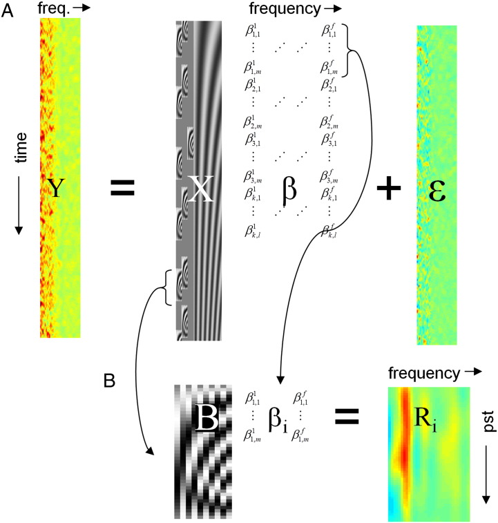
Fig. 1.

Schematic representation of the GLM approach for the analysis of time–frequency data.

A. Continuous time–frequency recording Y is modelled as the product of design matrix X and coefficients β with additive noise ε. X contains basis functions for each event and regressors modelling confounds (e.g. slow drifts). The GLM coefficients are estimated using ordinary or weighted least squares.

B. Event-type specific time–frequency images R_i are reconstructed by multiplying β_i—the GLM coefficients corresponding to the i-th event type—by the basis set B. These correspond to a least squares deconvolution of event-related responses from the original time-series.