Phase transitions in the first-passage time of scale-invariant correlated processes

Abstract

A key quantity describing the dynamics of complex systems is the first-passage time (FPT). The statistical properties of FPT depend on the specifics of the underlying system dynamics. We present a unified approach to account for the diversity of statistical behaviors of FPT observed in real-world systems. We find three distinct regimes, separated by two transition points, with fundamentally different behavior for FPT as a function of increasing strength of the correlations in the system dynamics: stretched exponential, power-law, and saturation regimes. In the saturation regime, the average length of FPT diverges proportionally to the system size, with important implications for understanding electronic delocalization in one-dimensional correlated-disordered systems.

I. INTRODUCTION

The dynamics of various complex systems are traditionally investigated by mapping them onto one-dimensional (1D) generalized random walks. The fundamental characteristics of random walks are represented by the statistical properties of first-passage time (FPT) [1], e.g., the functional form of its probability distribution and its average length. Empirical studies have reported a variety of forms for the probability distribution of FPT, including (i) pure exponential forms for random uncorrelated processes [2]; (ii) stretched exponential forms for a diverse group of natural and social complex systems ranging from neuron firing [3], climate fluctuations [4], or heartbeat dynamics [5], to Internet traffic [6,7] and stock market activity [8,9]; and (iii) a power-law form for certain on-off intermittency processes related to nonlinear electronic circuits [10] and anomalous diffusion [11–14]. Such diverse behavior is traditionally attributed to the specifics of the individual system. Identifying common factors responsible for similar behaviors of FPT across different systems has not been a focus of investigations. Indeed, these systems exhibit different scale-invariant long-range correlated behaviors, and how the degree of correlations embedded in the system dynamics relates to the statistical properties of FPT is not known. Here, we hypothesize that correlations are the unifying factor behind a class of complex systems of a diverse nature exhibiting similar statistical properties for FPT, and conversely, systems that belong to the same class of FPT properties possess a comparable degree of correlations. We investigate how the degree of correlations in the system dynamics affects key properties of FPT—the shape of the probability distribution P(ℓ) and the FPT average length 〈ℓ〉.

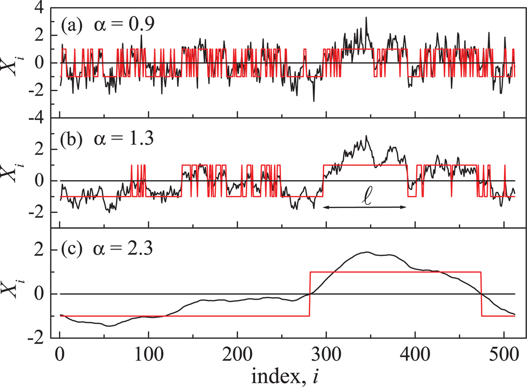
To investigate how the statistical properties of FPT depend on the degree of correlations in processes with scale-invariant dynamics, we use the inverse Fourier filtering method [15] to generate fractal signals with zero mean, unit standard deviation and the desired degree of long-range power-law correlations. The algorithm first generates a random signal in real space, then Fourier transforms it to the frequency (f) domain to obtain a white noise, multiplies this noise by a power law of the type f^{−(2α−1)/2}, and, finally, Fourier transforms the signal back into real space. Correlations in the resulting real-space signal are quantified by the exponent α, which, by construction, corresponds to the detrended fluctuation analysis (DFA) [16] scaling exponent (Fig. 1). The power spectrum S(f) of the resulting signal will be a power law of the form S(f) = 1/f^β, with β = 2α − 1. Given such a one-to-one relationship between the power spectrum exponent β and the DFA exponent α, we could have chosen any of them as our reference. However, we prefer to use as our reference the DFA exponent α, since the DFA method has become the standard when studying such long-range correlated time series [17–22], and can also be applied to real-world nonstationary signals. For uncorrelated random signals, α = 0.5; for anticorrelated signals, α < 0.5; and for positively correlated signals, α > 0.5. Processes with 0 < α < 1 are fractional Gaussian noises (fGns) and processes with 1 < α < 2 are fractional Brownian motions (fBms). In particular, α = 1.5 corresponds to the classical random walk. We will consider processes with α in the range 0 < α < 3, and for all such processes, the length ℓ of the FPT is defined as the distance between two consecutive zero crossings of the process (Fig. 1). Although, strictly speaking, the terminology of FPT is reserved for fBms (1 < α < 2), we will use it in the whole range of α (0 < α < 3) for simplicity.

FIG. 1.

(Color online) Examples of three scale-invariant processes (solid black line), each of system size N = 2⁹, and with different degree of correlations as quantified by the scaling exponent α obtained using the DFA method [16]. Increasing values of α indicate a higher degree of correlations. The first-passage time (FPT), defined as the interval ℓ between two consecutive zero crossings of the process, is indicated as segments of constant sign +1 or −1 (gray line). Note the change in the profile of the processes with increasing correlations leading to longer ℓ and to a corresponding change in the statistics of FPT.

II. FPT DISTRIBUTIONS

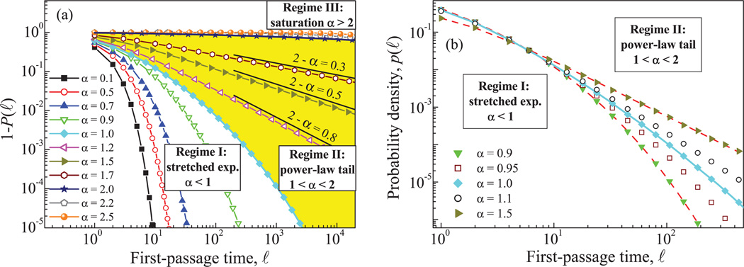
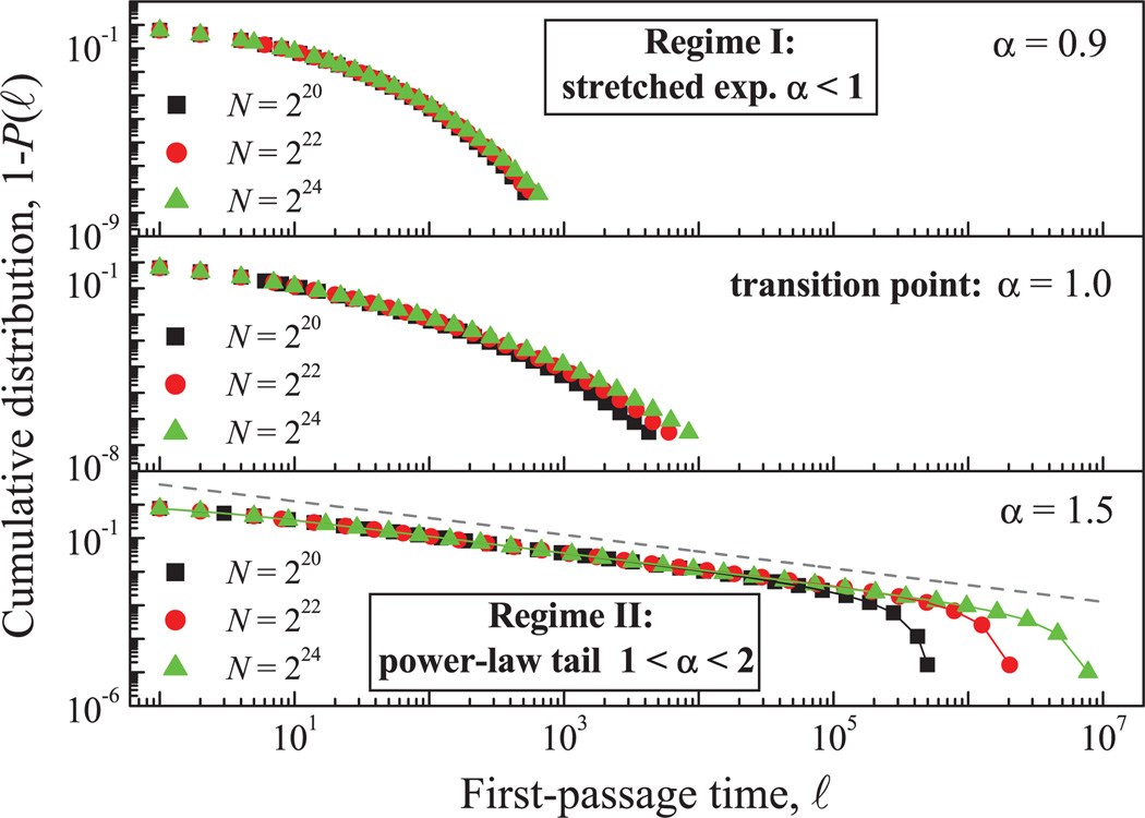
We obtain three different regimes [Fig. 2(a)] for the probability density p(ℓ) of the FPT length ℓ depending on the degree of correlations in the signal.

FIG. 2.

(Color online) (a) Cumulative probability distribution 1 − P(ℓ) of FPT intervals ℓ for scale-invariant processes with system size N = 2²⁴ and different degree of correlations quantified by the scaling exponent α. (b) Probability density p(ℓ) for small values of ℓ for processes close to the transition point α = 1. Dashed lines correspond to fittings with model (1) for α = 0.9, and with model (3) for α = 1.5.

A. Stretched exponential regime

For α < 1, we find that the probability density p(ℓ) behaves like a stretched exponential,

$$p(\ell )~\text{exp}[-{(\ell /{\ell }_0)}^{\epsilon }].$$ (1)

The stretching parameter ε depends on α: for the well-known case α = 0.5 (white noise), we find that ε = 1, corresponding to a pure exponential behavior. For α < 0.5, we find that ε > 1, and increases as α decreases. In this case, p(ℓ) decays faster than exponentially. For α > 0.5, we find that ε < 1, and decreases as α increases. In this case, p(ℓ) is a real stretched exponential and the tail of p(ℓ) becomes fatter as α increases. This result matches experimental observations for a great variety of phenomena [4,5,8,9] in this range of correlations, and is in agreement also with previous works in which fractal processes within this range of correlations are simulated and studied, as in Ref. [4], where the general result ε = 2 − 2α is numerically derived. Although the exact analytical derivation of the stretched exponential behavior in this regime is lacking, in Ref. [23], it was found that the stretched exponential form is an upper bound for the zero-level crossings (or the FPTs, as we name them here) in fGns, i.e., in the range 0 < α < 1.

B. Power-law tail regime

For 1 < α < 2, the model (1) is not valid, and we find that p(ℓ) behaves as

$$p(\ell )~\frac{f(\ell )}{{\ell }^{\delta }},$$ (2)

where the function f (ℓ) only affects the short-scale regime (small ℓ values), and tends to an unimportant constant as ℓ increases. Actually, f (ℓ) is responsible for the curvature of p(ℓ), which is appreciable at very short scales [Fig. 2(b)], and prevents the power-law divergence of (2) in the limit of small ℓ. However, the tail of the distribution behaves as a power law of exponent δ. We find numerically that the exponent δ and the correlation exponent α are related by δ = 3 − α. These results are in agreement with previous findings for the FPT distribution in this regime: although the exact analytical form of p(ℓ) is unknown, scaling arguments presented in [10], and a heuristic derivation shown in [12] based on results about the maximum value of a fBm [24], lead to a tail behavior such as the one in (2).

We find that the form of p(ℓ) and the relation between δ and α for the regime 1 < α < 2 generalize the particular well-known result corresponding to the FPT distribution of a random walk [2] (α = 1.5), where

$$p(\ell )~\frac{e^{-a/\ell }}{{\ell }^{3/2}}.$$ (3)

For α = 1, corresponding to 1/f noise, we find a transition between both regimes, where p(ℓ) presents an intermediate behavior and decays slower than (1) but faster than (2), as shown in Fig. 2(b).

C. Saturation regime

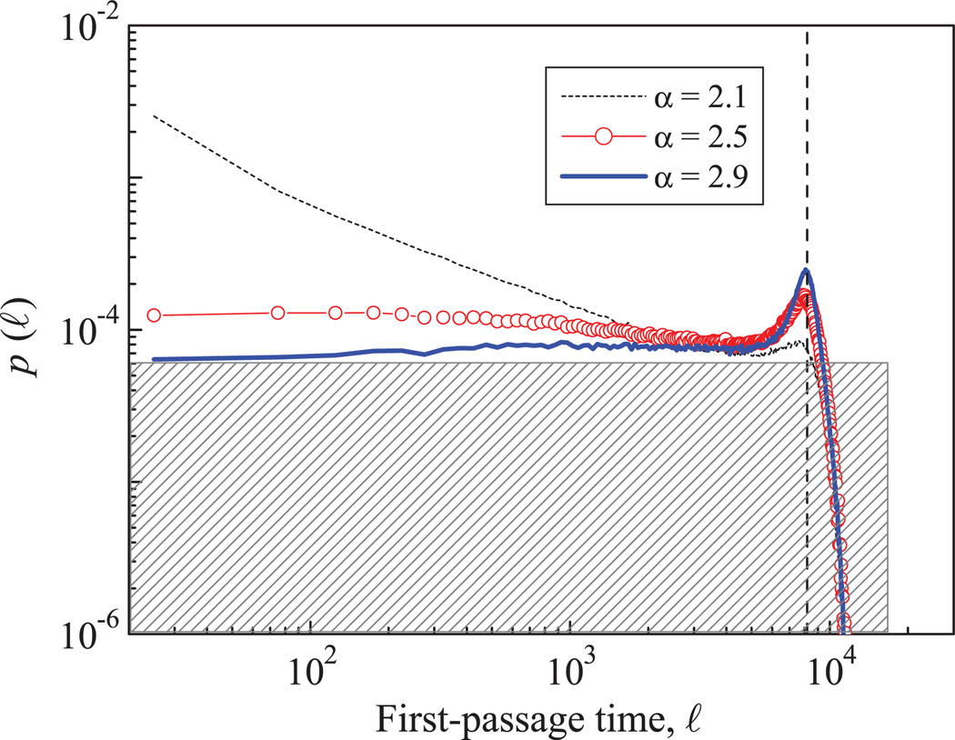
For α > 2, we should obtain δ = 3 − α < 1, and in this situation the probability density p(ℓ) cannot be normalized in the limit of large system size N. In this regime, p(ℓ) flattens for increasing α (Fig. 3) and tends to the constant probability density p(ℓ) = 1/N, shown with a shaded rectangle in Fig. 3. However, finite-size effects are very important, and a peak at ℓ = N/2 appears in p(ℓ), which becomes more pronounced as α increases. In practice, many of the FPTs are of the order of the system size and, correspondingly, the cumulative probability 1 − P(ℓ) is essentially flat independently of α [Fig. 2(a)].

FIG. 3.

(Color online) Probability densities p(ℓ) for processes with different α values in the saturation regime. The results correspond to a system size of N = 2¹⁴ and have been obtained with 10⁵ realizations for each α value. The shaded rectangle corresponds to the uniform distribution p(ℓ) = 1/N.

III. BEHAVIOR OF THE MEAN FPT

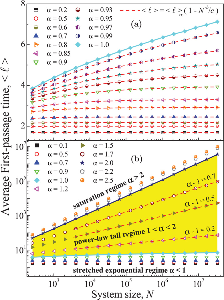
An important property that characterizes the distribution P(ℓ) is the average FPT, 〈ℓ〉. The behavior of 〈ℓ〉 as a function of the system size N is also different in the three regimes reported above (Fig. 4).

FIG. 4.

(Color online) (a)Convergent behavior of 〈ℓ〉 as a function of the system size N in the stretched exponential regime (α < 1). Dashed lines represent fittings with (4). (b) Dependence of 〈ℓ〉 on N for scale-invariant processes with different correlations for the three regimes we identified for P(ℓ) in Fig. 2. Note that panel (a) is a magnification of the bottom part of panel (b). Dashed lines in the power-law tail regime correspond to power-law fittings 〈ℓ〉 ~ N^γ, with γ = α − 1.

In the stretched exponential regime (α < 1), 〈ℓ〉 tends asymptotically to a finite constant value in the limit of large system size N [Fig. 4(a)]. In this regime, the behavior of 〈ℓ〉 as a function of N is well fitted [Fig. 4(a)] by a model of the type

$$\langle \ell \rangle ={\langle \ell \rangle }_{\mathrm{\infty }}(1-\frac{1}{{\mathit{\text{cN}}}^b})$$ (4)

where b and c are positive constants, and 〈ℓ〉_∞ represents the asymptotic value. Note that for increasing α, the convergence to the asymptotic value 〈ℓ〉_∞ is slower with the system size N, and the values of 〈ℓ〉_∞ also increase with α.

In the power-law tail regime (1 < α < 2), we find, in contrast [Fig. 4(b)], that 〈ℓ〉 diverges with the system size N as a power law,

$$\langle \ell \rangle ~N^{\gamma }.$$ (5)

This is in agreement with the fact that the tail of p(ℓ) follows a power law (2). Indeed, if (2) holds, then

$$\langle \ell \rangle ={\displaystyle {\int }_1^N}\ell p(\ell )d\ell ~{\displaystyle {\int }_1^N}\ell {\ell }^{-\delta }d\ell ~N^{2-\delta }.$$ (6)

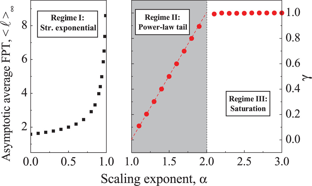
Thus, γ = 2 − δ, and since δ = 3 − α, we obtain γ = α − 1. Our numerical fits to the power laws in Fig. 4(b) provide γ values in agreement with this relation.

A phase transition from a convergent to a divergent behavior in the mean FPT 〈ℓ〉 is observed at α = 1 (Fig. 4). At this transition point, 〈ℓ〉 neither converges to a finite value, as in the stretched exponential regime, nor diverges as a power law with N, as in the power-law tail regime. We find that 〈ℓ〉 diverges logarithmically in the thermodynamic limit N → ∞: 〈ℓ〉 ~ log N.

In the saturation regime (α > 2), 〈ℓ〉 also diverges with the system size N as a power law, but with a constant exponent γ = 1 for all α values [Fig. 4(b)], i.e., 〈ℓ〉 ~ N. Note that 〈ℓ〉 cannot grow faster than the system size N, thus precluding γ > 1 values.

At the transition point between the power-law tail and the saturation regime (α = 2), we find that 〈ℓ〉 ~ N / log N. This behavior is intermediate between both regimes: 〈ℓ〉 increases faster than any power law with γ < 1, but slower than a power law with γ = 1 [Fig. 4(b)].

The behavior of 〈ℓ〉 in the thermodynamic limit can be summarized in a phase diagram as shown in Fig. 5. In the stretched exponential regime (left panel in Fig. 5), where 〈ℓ〉 converges in the thermodynamic limit, the natural choice of the order parameter is the asymptotic value 〈ℓ〉_∞, which increases with α and diverges when α → 1⁻. In the other two regimes (right panel in Fig. 5), as 〈ℓ〉 diverges with N as 〈ℓ〉 ~ N^γ, a convenient order parameter to describe the behavior of 〈ℓ〉 is the exponent γ, which tends to zero as α → 1⁺ and converges to γ = 1 as α → 2⁻. In the saturation regime α > 2, the order parameter remains constant: γ = 1. The main properties of 〈ℓ〉 and the probability density p(ℓ) in the three regimes are also summarized in Table I.

FIG. 5.

(Color online) Phase diagram of the transitions from stretched exponential to power-law tail to saturation regime. Symbols correspond to numerical results, and the dashed line corresponds to the curve γ = α − 1. For α < 1 (left panel), the order parameter is the asymptotic value 〈ℓ〉_∞ [Fig. 3(a)], while for α > 1 (right panel), the order parameter is the exponent γ of Eq. (5).

TABLE I.

Properties of the probability density p(ℓ) and the average FPT length 〈ℓ〉 in the three different regimes that we find as a function of the DFA correlation exponent α.

α	p(ℓ)	〈ℓ〉
Regime I (stretched exp.)	~exp[−(ℓ/ℓ0)2−2α]	limN→∞〈ℓ〉 = 〈ℓ〉∞, constant for fixed α
0 < α < 1		〈ℓ〉∞ increases with α
Regime II (power-law tail)	~1/ℓ3−α	~Nα−1
1 < α < 2
Regime III (saturation)	flattens with α	~N
2 < α < 3	strong size effects at ℓ = N/2

The results we obtain for the behavior of 〈ℓ〉 in the three regimes can also be understood in terms of the finite-size effects of the distribution P(ℓ) (Fig. 6). For processes with α < 1, P(ℓ) is essentially independent of the system size N. Thus, the mean FPT 〈ℓ〉 is well defined and, for large enough N, there are no appreciable size effects, giving rise to a finite asymptotic value 〈ℓ〉_∞ [Fig. 4(a)]. At the transition point α = 1, where the 〈ℓ〉 diverges logarithmically [Fig. 4(a)], the system-size effects on P(ℓ) become more pronounced (Fig. 6, middle panel). Above the transition point α > 1, for any finite realization, there is a cutoff in the power-law tail of P(ℓ) which scales with the system size N (Fig. 6, bottom panel), ensuring the power-law tail of the distribution even in the thermodynamic limit N → ∞, and thus 〈ℓ〉 diverges as a power law of N [Fig. 4(b)].

FIG. 6.

(Color online) Dependence of the cumulative distributions 1 − P(ℓ) on the system size N. The transition from the stretched exponential to the power-law regime is stable and independent of N. The distributions shown in all panels are obtained by Monte Carlo simulations with 2³²/N realizations.

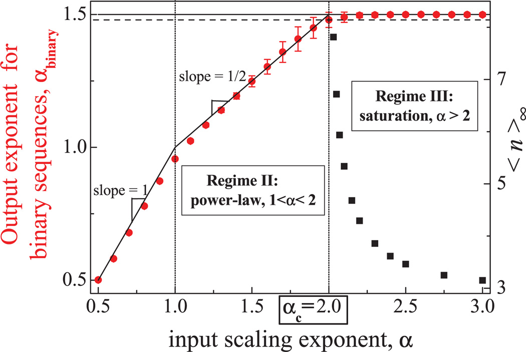
Another important quantity related to the dependence of the FPT statistics with the system size N is the average number of FPT segments, 〈n〉. Segments are defined as continuous parts of the process with constant sign, the borders of which are the zero crossings (Fig. 1). We find that the behavior of 〈n〉 in the three regimes (not shown) is essentially the inverse of 〈ℓ〉: in the stretched exponential regime, 〈n〉 diverges as 〈n〉 ~ N independently of α. In the power-law tail regime, 〈n〉 diverges more slowly 〈n〉 ~ N^λ, where the exponent λ = 2 − α decreases when α → 2⁻. Finally, in the saturation regime (α > 2), 〈n〉 converges with N → ∞ to an asymptotic constant value 〈n〉_∞, which decreases with increasing α.

In conclusion, correlations can be seen as the unifying factor controlling the statistical properties of FPTs in a large class of fractal processes, irrespective of the specifics of the particular dynamical system considered. When correlations are in the range α < 1 (such as in climate records [4] or stock market activity [8,9]), FPTs probability density p(ℓ) behaves as stretched exponentials, with a finite mean value even for diverging system sizes. In contrast, when correlations are in the range 1 < α < 2, as, for example, in anomalous diffusion processes [11–14], p(ℓ) follows a power law in the tail, p(ℓ) ~ ℓ^−δ with δ = 3 − α, generalizing the results for the classical random walk (α = 3/2), for which δ = 3/2. In this case, the FPT mean value increases as a power law of the system size with an exponent smaller than one. For the case of processes with extreme correlations (2 < α < 3), which can be seen as integrations of fBms, the probability densities p(ℓ) are essentially flat, and the FPT mean value diverges with the system size.

IV. IMPLICATIONS TO CORRELATED-DISORDERED SYSTEMS

The results obtained here are closely related to the behavior of binary signals: a standard technique to generate binary correlated fractal processes is to simply consider the sign of the underlying continuous fractal process. In this way, binary sequences are obtained that are composed of segments of only two possible values, either +1 or −1. The sizes of these segments are the FPTs of the original signal (Fig. 1). This kind of binary sequence occurs in systems of diverse nature, such as seismic signals [25], membrane transport [26], DNA chains [19,27], and disordered binary solids [28,29].

In particular, our findings for the statistical properties of FPTs can explain earlier observations for the electronic properties of correlated 1D disordered systems. It has been observed that the strength of the long-range correlations in such systems can control their electronic properties, as the localization length [30–32] or the level statistics [33]. For 1D binary systems, α = 0.5 corresponds to the random binary alloy [34], where the electronic states are exponentially localized. However, when positive correlations (α > 0.5) are introduced in binary systems, a delocalization effect is observed [29]. This latter effect can be understood in terms of our results presented here, as we explain below.

In 1D binary systems, the FPTs correspond to the sizes of ordered regions —patches with the same type of atoms. Since electrons are typically able to move within these patches, we expect the average localization length 〈λ〉 to be proportional to the average patch size 〈ℓ〉: 〈λ〉 ~ 〈ℓ〉. Therefore, in the stretched exponential regime α < 1, the localization length 〈λ〉 ~ 〈ℓ〉_∞ is essentially constant and independent of the system size N, which is a typical feature of localized electrons in disordered systems corresponding to insulating behavior [29]. In the power-law tail regime (1 < α < 2), we expect 〈λ〉 ~ N^γ, where γ = α − 1. Since the localization length increases as a power law of the system size N, there is a correlation-induced delocalization effect. However, the fraction of the system occupied by the state, 〈λ〉/N, behaves as 〈λ〉/N ~ N^α−2 and tends to zero (1 < α < 2) in the thermodynamic limit, i.e., the wave functions are still localized.

In contrast, in the saturation regime α > 2, we find ℓ ~ N [Fig. 3(b)]. In this case, the system consists of a finite number of patches 〈n〉_∞, which is independent of the system size N, and the patches are macroscopically large in the thermodynamic limit, N → ∞. In this regime, we expect 〈λ〉 ~ N, and the electronic wave function to be extended (typically within one of the macroscopic patches), giving rise to a conducting behavior. Thus, at the critical point α = 2, we expect a transition from a localized to an extended electronic behavior.

Such a localized-extended transition was presented in [29], where the localization length λ as a function of the correlations present in the binary sequence was studied. In [29], correlations were measured with the DFA scaling exponent calculated directly in the binary sequences (α_binary), and not with the scaling exponent α of the underlying continuous fractal process. The transition presented in [29] was reported to occur at α_binary ≃ 1.45, and was interpreted as a metal-insulator transition driven by the degree of correlations in disordered 1D binary systems, which is in contradiction to the Anderson localization theory that asserts that 1D disordered solids can behave only as insulators.

However, a value of α_binary ≃ 1.45 as measured by the DFA method in the binary sequence corresponds to a value of α = 2 that is embedded in the underlying continuous fractal process from which the binary sequence has been obtained (Fig. 7). Thus, the critical point reported in [29] corresponds to the transition presented here at α = 2 from the power law to the saturation regime (Fig. 5), and thus the conducting phase reported in [29] obtained for α_binary > 1.45 corresponds to the saturation regime presented here (α > 2), where the system is actually not disordered but is composed of a finite and fixed number (〈n_∞〉; see Fig. 7) of patches, which will be macroscopically large in the thermodynamic limit, giving rise to an ordered state with conducting behavior. Therefore, at the critical point α = 2 (or α_binary = 1.45), the system is not a disordered system undergoing an insulator-metal transition driven by the correlations (as claimed in [29]), but a system which undergoes a disordered-ordered transition driven by the correlations.

FIG. 7.

(Color online) We show the DFA scaling exponent α_binary (red circles) obtained in binary sequences mapped from real-valued long-range correlated processes as a function of the α values of the latter. For the case α > 2, we also show the asymptotic average number of patches (black squares) forming the system, 〈n〉_∞ (right axis). All the numerical results have been obtained for a system size of N = 2²², and with 1024 realizations. The vertical dotted lines show the transition between the three different regimes, at α = 1 and α = 2. The horizontal dashed line close to α_binary = 1.5 corresponds to α_binary = 1.45, and is the value reported in [29] at which a metal-insulator transition was observed. Note how the dependence of α_binary on α is different in the three regimes presented here.

References

- 1.Condamin S, Bénichou O, Tejedor V, Voituriez R, Klafter J. Nature (London) 2007;450:77. doi: 10.1038/nature06201. [DOI] [PubMed] [Google Scholar]
- 2.Bunde A, Havlin S, editors. Fractals in Science. Berlin: Springer-Verlag; 1995. [Google Scholar]
- 3.Schindler M, Talkner P, Hänggi P. Phys. Rev. Lett. 2004;93:048102. doi: 10.1103/PhysRevLett.93.048102. [DOI] [PubMed] [Google Scholar]
- 4.Bunde A, Eichner JF, Kantelhardt JW, Havlin S. Phys. Rev. Lett. 2005;94:048701. doi: 10.1103/PhysRevLett.94.048701. [DOI] [PubMed] [Google Scholar]
- 5.Reyes-Ramírez I, Guzmán-Vargas L. Europhys. Lett. 2010;89:38008. [Google Scholar]
- 6.Leland WE, et al. IEEE ACM Trans. Network. 1994;2:1. [Google Scholar]
- 7.Cai SM, et al. Europhys. Lett. 2009;87:68001. [Google Scholar]
- 8.Ivanov PCh, Yuen A, Podobnik B, Lee Y. Phys Rev. E. 2004;69:056107. doi: 10.1103/PhysRevE.69.056107. [DOI] [PubMed] [Google Scholar]
- 9.Wang FZ, Yamasaki K, Havlin S, Stanley HE. Phys. Rev. E. 2009;79:016103. doi: 10.1103/PhysRevE.79.016103. [DOI] [PubMed] [Google Scholar]
- 10.Ding MZ, Yang WM. Phys. Rev. E. 1995;52:207. [Google Scholar]
- 11.Shlesinger MF, Zaslavsky GM, Klafter J. Nature (London) 1993;363:31. [Google Scholar]
- 12.Rangarajan G, Ding MZ. Phys. Lett. A. 2000;273:322. [Google Scholar]
- 13.Khoury M, Lacasta AM, Sancho JM, Lindenberg K. Phys. Rev. Lett. 2011;106:090602. doi: 10.1103/PhysRevLett.106.090602. [DOI] [PubMed] [Google Scholar]
- 14.Eliazar I, Klafter J. Phys. Rev. E. 2009;79:021115. doi: 10.1103/PhysRevE.79.021115. [DOI] [PubMed] [Google Scholar]
- 15.Makse HA, Havlin S, Schwartz M, Stanley HE. Phys. Rev. E. 1996;53:5445. doi: 10.1103/physreve.53.5445. [DOI] [PubMed] [Google Scholar]
- 16.Peng C-K, Buldyrev SV, Havlin S, Simons M, Stanley HE, Goldberger AL. Phys. Rev. E. 1994;49:1685. doi: 10.1103/physreve.49.1685. [DOI] [PubMed] [Google Scholar]
- 17.Hu K, Ivanov PC, Chen Z, Carpena P, Stanley HE. Phys. Rev. E. 2001;64:011114. doi: 10.1103/PhysRevE.64.011114. [DOI] [PubMed] [Google Scholar]
- 18.Coronado AV, Carpena P. J. Biol. Phys. 2005;31:121. doi: 10.1007/s10867-005-3126-8. [DOI] [PMC free article] [PubMed] [Google Scholar]
- 19.Carpena P, Bernaola-Galvan P, Coronado AV, Hackenberg M, Oliver JL. Phys. Rev. E. 2007;75:032903. doi: 10.1103/PhysRevE.75.032903. [DOI] [PubMed] [Google Scholar]
- 20.Blázquez MT, et al. Physica A. 2009;388:1857. [Google Scholar]
- 21.Xu YL, et al. Physica A. 2011;390:4057. doi: 10.1016/j.physa.2011.05.015. [DOI] [PMC free article] [PubMed] [Google Scholar]
- 22.Ma QDY, Bartsch RP, Bernaola-Galvan P, Yoneyama M, Ivanov PC. Phys. Rev. E. 2010;81:031101. doi: 10.1103/PhysRevE.81.031101. [DOI] [PMC free article] [PubMed] [Google Scholar]
- 23.Newell GF, Rosemblatt M. Ann. Math. Stat. 1962;63:1306. [Google Scholar]
- 24.Molchan GM. Commun. Math. Phys. 1999;205:97. [Google Scholar]
- 25.Varotsos PA, Sarlis NV, Skordas ES. Phys. Rev. E. 2003;67:021109. doi: 10.1103/PhysRevE.67.021109. [DOI] [PubMed] [Google Scholar]
- 26.Varotsos PA, Sarlis NV, Skordas ES. Phys. Rev. E. 2003;68:031106. doi: 10.1103/PhysRevE.68.031106. [DOI] [PubMed] [Google Scholar]
- 27.Carpena P, Oliver JL, Hackenberg M, Coronado AV, Barturen G, Bernaola-Galvan P. Phys. Rev. E. 2011;83:031908. doi: 10.1103/PhysRevE.83.031908. [DOI] [PubMed] [Google Scholar]
- 28.Usatenko OV, et al. Physica A. 2008;387:4733. [Google Scholar]
- 29.Carpena P, et al. Nature (London) 2002;418:955. doi: 10.1038/nature00948. [DOI] [PubMed] [Google Scholar]
- 30.de Moura FABF, Lyra ML. Phys. Rev. Lett. 1998;81:3735. [Google Scholar]
- 31.Izrailev FM, Krokhin AA. Phys. Rev. Lett. 1999;82:4062. doi: 10.1103/PhysRevLett.100.126402. [DOI] [PubMed] [Google Scholar]
- 32.Esmailpour A, Esmaeilzadeh M, Faizabadi E, Carpena P, Tabar MRR. Phys. Rev. B. 2006;74:024206. [Google Scholar]
- 33.Carpena P, Bernaola-Galván P, Ivanov PCh. Phys. Rev. Lett. 2004;93:176804. doi: 10.1103/PhysRevLett.93.176804. [DOI] [PubMed] [Google Scholar]
- 34.Davids PS. Phys. Rev. B. 1995;52:4146. doi: 10.1103/physrevb.52.4146. [DOI] [PubMed] [Google Scholar]