Population Rate Dynamics and Multineuron Firing Patterns in Sensory Cortex

Abstract

Cortical circuits encode sensory stimuli through the firing of neuronal ensembles, and also produce spontaneous population patterns in the absence of sensory drive. This population activity is often characterized experimentally by the distribution of multineuron “words” (binary firing vectors), and a match between spontaneous and evoked word distributions has been suggested to reflect learning of a probabilistic model of the sensory world. We analyzed multineuron word distributions in sensory cortex of anesthetized rats and cats, and found that they are dominated by fluctuations in population firing rate rather than precise interactions between individual units. Furthermore, cortical word distributions change when brain state shifts, and similar behavior is seen in simulated networks with fixed, random connectivity. Our results suggest that similarity or dissimilarity in multineuron word distributions could primarily reflect similarity or dissimilarity in population firing rate dynamics, and not necessarily the precise interactions between neurons that would indicate learning of sensory features.

Introduction

Cortical activity, like animal behavior, has a probabilistic character (Rao et al., 2002). Recordings of single cells have shown that presentation of an identical stimulus can cause variable responses from one presentation to the next; yet the probabilistic sensory responses of any one neuron are a manifestation of a more complex distribution of activity at the population level. Furthermore, even in the absence of sensory stimuli, the cortex produces unpredictable but structured spontaneous activity that in many ways resembles sensory responses (Kenet et al., 2003; Fiser et al., 2004; DeWeese and Zador, 2006; Okun and Lampl, 2008; Luczak et al., 2009; Ringach, 2009; Tkacik et al., 2010). Characterizing the structure and function of this probabilistic activity is an essential step toward understanding how neuronal populations process information.

One of the most intriguing interpretations of the probabilistic nature of neural activity is the “sampling-based representation” hypothesis (Hoyer and Hyvarinen, 2003; Fiser et al., 2010). Psychophysical experiments indicate that the brain acquires probabilistic models of the external environment (Knill and Richards, 1996; Ernst and Banks, 2002; Kersten et al., 2004; Franklin and Wolpert, 2011; Moreno-Bote et al., 2011). The sampling hypothesis holds that these models are explicitly represented as probability distributions over neuronal spikes or membrane potentials, with the parameters of the distribution encoded in synaptic weights, and learned via experience-dependent synaptic plasticity. This internal model causes population responses to represent samples from a posterior distribution given a particular sensory input.

A recent study in primary visual cortex appeared to support this sampling hypothesis (Berkes et al., 2011). By representing population activity as N-bit binary words, this study found that word distributions during spontaneous activity are similar to those elicited by presentation of natural movie clips in adult ferrets, but not in juveniles; furthermore, in adults, spontaneous word distributions matched those of natural movies but not artificial drifting gratings. This is indeed what one would expect to find if V1 responses were generated by a sampling-based internal model of the natural visual world acquired during development.

Here we show that similarities and differences between cortical word distributions are dominated not by precise interactions between units (as would be expected from the sampling hypothesis), but by variations in the dynamics of population rate: the instantaneous summed activity of all neurons in the population. Fluctuations in population rate are one of the most prominent features of cortical activity. The strength of these fluctuations varies as a function of cortical state, from strongly fluctuating activity in synchronized states such as slow-wave sleep, to steadier activity found in more desynchronized states such as active behavior (Poulet and Petersen, 2008; Okun et al., 2010). We introduce a simple phenomenological model for word distributions (the “raster marginals model”), parameterized by measures of population rate dynamics rather than by precise interactions between units. This model accounts for similarities between multineuron word distributions in primary auditory and visual cortex of anesthetized rats and cats, as well as in artificial networks of integrate-and-fire neurons. It also captures the experimental findings that appeared to support the sampling hypothesis (Berkes et al., 2011), questioning the use of multineuron word distributions to characterize the learning of sensory features.

Materials and Methods

Recordings in rat A1.

Experiments were performed at Rutgers University in accordance with protocols approved by the Animal Care and Use Committee. The experimental details and the data used here were previously described in Marguet and Harris, 2011. Briefly, male Sprague Dawley rats were anesthetized with urethane plus supplemental doses of ketamine and xylazine. This anesthesia regime produced robust and well controlled switches between synchronized and desynchronized states, which either occurred spontaneously or were induced by tail pinch, and could be detected both in the local field potential (LFP) spectrogram and in the coefficient of variation (CV) of the population rate (see below).

Silicon probes (32 contacts) arranged in an eight tetrode configuration (NeuroNexus Technologies) were advanced into layers V and VI of the left primary auditory cortex (A1). Signals were amplified, digitized at 20 kHz, and stored for off-line analysis. The auditory stimulus consisted of 30–50 s intervals of amplitude-modulated noise. Stimulus presentations were separated by intervals of silence of equal duration, in which spontaneous activity was recorded.

Spikes were detected and visually verified using the programs NDmanager and Neuroscope (Hazan et al., 2006). In the original study by Marguet and Harris (2011) the spikes on each tetrode were sorted; here, instead, we followed the analysis methods of Berkes et al. (2011), and simply accumulated all unsorted spikes from each tetrode.

To quantify cortical state, we adopted the measure of Renart et al. (2010), based on the CV of the population rate. We considered 10 s intervals of spontaneous activity and divided them into 200 windows of 50 ms each. For each window, we determined the population rate, i.e., the total number of spikes on all the tetrodes. We took the CV of population rate over the 200 windows as the measure of cortical state in that time interval. We considered values of CV ≥ 1 to indicate synchronized states and CV ≤ 0.5 to indicate a desynchronized state (see Fig. 1C).

Figure 1.

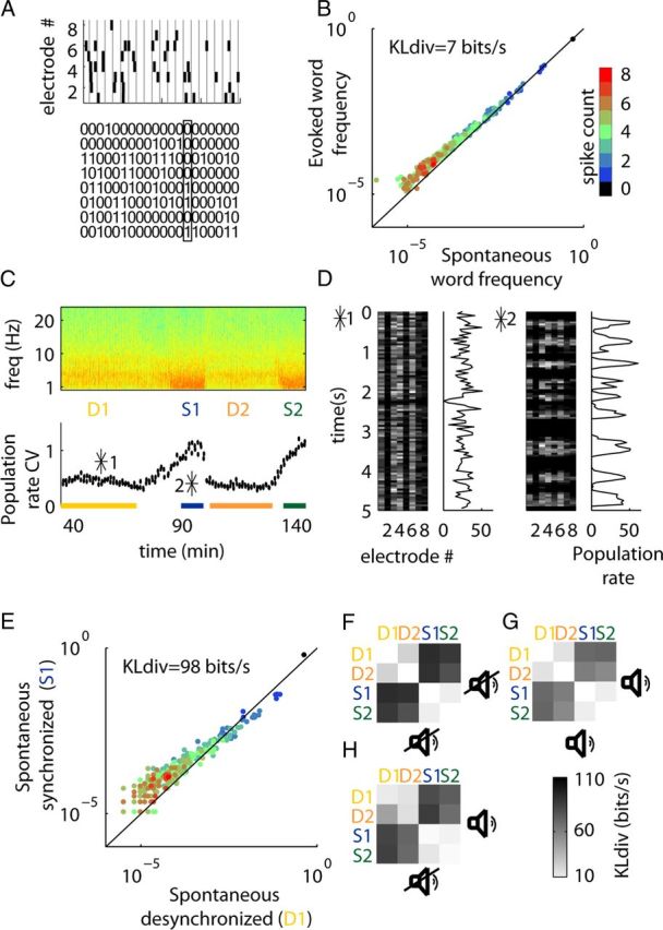
Word distributions in rat A1 are state dependent. A, The multiunit spiking activity on eight tetrodes was converted into a binary matrix whose columns represent the presence of spikes in consecutive, nonoverlapping 2 ms bins. B, Spontaneous and stimulus-evoked word distributions are similar when accumulated over the whole dataset. The plot shows the probability of every 8-bit word, with color representing the number of 1s it contains. C, Cortical states. Top, Spectrogram of LFP on one electrode. Bottom, Running CV of the population rate, computed from 10 s intervals of spontaneous activity (see Materials and Methods). The CV and low-frequency power are substantially higher in synchronized-state epochs (S1 and S2). D, Example rasters of spontaneous activity during desynchronized and synchronized states (the position of these intervals within the recording shown in C is indicated by asterisks). The corresponding population rate (spikes/50 ms bin) is shown to the right of each raster. E, The spontaneous word distribution differs between states. F, Pseudocolor matrix showing KLdiv between spontaneous word distributions in each pair of periods. The distributions are similar within states, but different across states. G, H, Same plot as in F, for evoked-evoked and spontaneous-evoked word distributions.

We analyzed data from three animals. In rats 1 and 2 we detected two stable epochs of both synchronized and desynchronized activity (Fig. 1C); extracting spontaneous and sensory-evoked data from these four epochs provided eight segments of activity for our analysis. In rat 3, the amplitude modulated noise stimulus spanned only one period of synchronized and desynchronized states; however, spontaneous activity was recorded in additional periods of both synchronized and desynchronized states, leading in total to six instead of eight segments.

Recordings in cat V1.

Experiments were conducted at the Smith–Kettlewell Eye Research Institute in accordance with protocols approved by the Institutional Animal Care and Use Committee. The experimental details and the data used here were previously described in Benucci et al., 2009 and Busse et al., 2009. Briefly, female cats were anesthetized with ketamine and xylazine for initial surgery, followed by sodium pentothal and fentanyl for electrophysiological recordings. The signals from 96-channel multi-electrode (Utah) array were recorded using the Cerebus 128-channel system (Blackrock Microsystems). The recordings were primarily from layers II and III. Spikes were detected on-line by a threshold set to ∼3–4 SD of the background noise. The spike waveforms were digitized at 30 kHz and stored for off-line analysis. Only electrodes that detected spiking activity were used in this analysis.

Estimation of the Kullback–Leibler divergence between word distributions.

The firing patterns recorded by a multi-electrode array were described by N-bit words, where a word represents the presence of a spike on each of the N electrodes (N = 8 for rat A1; N = 16 for cat V1) in a brief interval (2 ms). In this representation the match between any two kinds of activity recorded on the same electrodes is quantified by the Kullback–Leibler divergence (KLdiv, measured in bits/s) between the two distributions of 2^N values.

Throughout the paper we use the symmetrized version of KLdiv, given by D_s[P||Q] = (D[P||Q] + D[Q||P])/2, unless stated otherwise. To estimate KLdiv between two experimentally observed or synthetically generated word distributions, we used the symmetrized form of the Bayesian, bias-corrected estimator introduced in Berkes et al., 2011; Equations S12–S14 of their supplemental material. To express the KLdiv in bits, the value was normalized by a log(2) factor. To verify that this estimator provides accurate results when the number of the available samples for each of the two distributions is different, e.g., as in the case of Figure 1F–H, we used synthetic rasters drawn from pairs of word distributions whose true KLdiv was computed analytically (data not shown).

The raster marginals model.

The raster marginals model (see Fig. 2B) synthesizes a random population raster with a specified mean firing rate (MFR) for each electrode and a specified population rate distribution (PRd). To operate, the algorithm must be given: (1) the number of time bins T of the raster that is to be synthesized, (2) the total number of spikes S_i occurring on electrode i during this duration for all i between 1 and the number of electrodes N, and (3) the total number of time bins r_i for which the instantaneous Population Rate (i.e., the total spike count for that time bin, summed over all electrodes) was i, for all i between 0 and N. Note that ∑_i=0^Nr_i = T is the total number of time bins. Since it must hold that ∑_i=1^NS_i = ∑_i=0^Ni · r_i, the model is described by 2N parameters. These parameters determine the two marginals of a binary matrix of dimensions N-by-T, up to a permutation of the columns (Fig. 2B).

Figure 2.

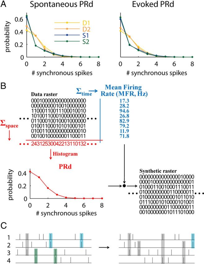
The raster marginals model. A, PRd of spontaneous and evoked activity in each of the recording intervals shown in Figure 1C. B, Illustration of the model. Summing the rows of the raster matrix provides the mean firing rate (MFR) for each electrode. Summing columns provides the population rate, whose distribution (PRd) is used by the model. MFR and PRd summarize the raster by 2N parameters, which are used to produce a synthetic raster (see Materials and Methods). C, Illustration of a correlation structure that cannot be captured by the model. Left, Spike coincidences predominantly occur between units 1–2 (blue) and 3–4 (green), whereas all other coincidences are rare (gray). Right, In the output produced by the model, coincident spikes occur between any pair of units.

In general, there are many different matrices with the given marginals. To construct one, we can begin with some random matrix that satisfies (3), and by repeatedly shifting 1s within the same column from any row i whose sum exceeded S_i into a row j whose sum fell below S_j, bring it to satisfy (2) as well. An alternative approach is to use Ryser's (deterministic) algorithm to construct the canonical matrix with such marginals (Ryser, 1957, 1960; Brualdi, 2006). Once we have a matrix with the specified marginals, it can be randomized by repeatedly picking a 2 × 2 submatrix in which each row and each column contains 0 and 1, and switching between the 0s and 1s. It is possible to move between any two 0/1 matrices having the same marginals (modulo column permutation) by a sequence of applications of this operation (Ryser, 1957). Consecutive application of a shift in a randomly chosen 2 × 2 submatrix can be used to get in the limit a uniform distribution over all matrices with given marginals (Rao et al., 1996). In our particular case of matrices that have many columns but few rows, this can be significantly sped up by applying the shift operation in parallel on multiple 2 × 2 submatrices from the same pair of rows.

To the best of our knowledge, the raster marginals model represents the first application to neuroscience of the combinatorial theory of 0/1 matrices with given marginals. The model is related to a raster shuffling method in which pairs of spikes in different trains are exchanged (Luczak et al., 2007; Grün, 2009). There is, however, an important conceptual difference between the two—unlike shuffling, the model gets no knowledge about the original raster beyond the 2N parameters. Thus, one need not be concerned with the potential problem of some structure in the original data not being destroyed by shuffling. One additional difference is that shuffling preserves the temporal dynamics of population rate of the original raster, whereas the model cannot.

For an empirically observed word distribution P, we use P̂ to denote the word distribution produced by the raster marginals model given the parameters corresponding to P. We use P̃ for the word distribution constructed by retaining the MFRs of the original data but assuming each spike train is independent of the others.

Estimating properties of the PRd.

In many recordings the PRd resembles the lognormal (see Results). As the support of the lognormal distribution is real numbers >0, whereas spike counts are integers including 0, to fit a lognormal distribution to the observed PRds, we shifted the measured spike counts upward by 1, and further added a “noise” value, uniformly distributed between 0 and 1, to the number of spikes in each bin. We evaluated the quality of the shifted lognormal fit by the KLdiv between the observed distribution and the fit. Specifically, if P(r) denotes the observed probability to have r simultaneous spikes in a 2 ms bin and Q(r) is this probability according to the fit, its quality is given by the following:

where the factor of 500 is used to obtain the units of bits/s (from a 2ms bin size), and M is the maximal number of simultaneous spikes observed at least 30 times in the given block. In our V1 data M was on average 48 ± 14. The upper limit on r is required because P(r) cannot be reliably estimated when r is close to 96: as r approaches this value, the occurrence of r simultaneous spikes becomes increasingly rare.

To estimate the KLdiv between PRds of pairs of recording segments, we used the symmetrized version of the above formula. We used this direct estimate instead of the Bayesian bias-corrected estimator (used for word distributions) because the number of different r values does not grow exponentially with N (r is distributed over N + 1 values at most, whereas w is distributed over 2^N values), hence the probabilities can be estimated accurately from the limited amount of available empirical data.

Several theoretical papers derived an analytical expression for the PRd (Amari et al., 2003; Macke et al., 2011). However, the assumptions made in these works seem too restrictive for our application. In our case an additional complication with using these results arises because the multiunit signal on each electrode consists of spike trains from an unknown number of neurons surrounding it.

To simulate ferret data according to the raster marginal model (see Fig. 7B–D), we used shifted lognormal PRds with parameters specified in Table 1. These values are within the same range as those observed in the data from cat V1 (data not shown). As these values provide PRd for rasters of 96 channels rather than 16, we downsampled the distribution by computing the expectation for the number of spikes on 16 channels given that there were i spikes in total (for every 96 ≥ i ≥ 0).

Figure 7.

Changes in population rate dynamics can explain increasing similarity of spontaneous and evoked word distributions with development. A, The key experimental findings of Berkes et al., 2011. Top, KLdiv between spontaneous spiking activity [S], and activity during presentation of natural movies [M] in juvenile and adult ferrets. Bottom, KLdiv between the word distributions in actual data [M or S] and the word distributions predicted by MFR alone [M̃ or S̃, respectively]. B, Parameters of the raster marginals model used to reproduce the data in A. Top, MFRs on 16 electrodes. The MFRs of the 16 “S” (“spontaneous”) spike trains were drawn from a normal distribution with μ = 20 spikes/s, σ = 15 spikes/s, and μ = 60 spikes/s, σ = 45 spikes/s, for “juveniles” and “adults,” respectively. The “M” (“natural movie”) rates were obtained by multiplying the spontaneous rate of each spike train by a coefficient drawn from a normal distribution with μ = 2, σ = 0.5, and μ = 1.25, σ = 0.125, for juveniles and adults, respectively. Bottom, PRds, taken to be shifted lognormal as in cat V1 (see Materials and Methods). Blue and green points indicate parameters used to create synthetic juvenile and adult rasters, respectively. C, Comparison of the spontaneous and evoked word distributions produced by the model for the juvenile (top) and adult (bottom) conditions. D, Summary statistics for the raster marginals model, shown in the same format as A. Error bars indicate SDs over 100 repeats, one of which is shown in B and C.

Table 1.

Parameters for simulated PRds

	“S”	“M”
“Juvenile”	μ = 1.5, σ = 0.6	μ = 2.05, σ = 0.6
“Adult”	μ = 2.275, σ = 0.8	μ = 2.48, σ = 0.8

Simulations of random recurrent spiking network.

To demonstrate that similarity of spontaneous and evoked word distributions can occur without learning, we simulated a network of 10,000 conductance-based integrate-and-fire neurons, of which 80% were excitatory and 20% inhibitory. The network was implemented with the NEST simulator (Gewaltig and Diesmann, 2007), accessed via the PyNN interface (Davison et al., 2008). The time step of the simulations was 0.1 ms.

The membrane potential V of the neurons followed exponential integrate-and-fire dynamics (Brette and Gerstner, 2005; Destexhe, 2009):

Here C_m is the cell's capacitance; g_e(t) and g_i(t) are the total excitatory and inhibitory conductances due to synaptic input; E_e and E_i are excitatory and inhibitory reversal potentials; g_L is the leak conductance; E_L is the resting potential; V_T is spike approach threshold; Δ controls the steepness of approach to spike threshold. Spiking was triggered at a threshold of −40 mV, following which V was clamped at −70 mV for the following 5 ms. V was prevented from going below −80 mV by a hard lower bound. The current w in the above equation models spike-frequency adaptation observed in cortical neurons, and is governed by the following:

where τ_w is the time constant of w, and a controls adaptation strength. After every spike w increases by b nA.

The neurons were randomly connected with connection probability of 2% between E-E, E-I, I-E, and I-I pairs. The synaptic conductances were represented by α functions, with excitatory synapses having a peak strength of 6 nS and time constant of τ_e, while the corresponding values for inhibitory synapses were 40 nS and τ_i. The axonal conductance delays were drawn randomly and uniformly between 0.2 and 3 ms.

To enforce heterogeneity across neurons, some of these parameters (bold in Table 2) were drawn from Gaussian distributions whose means and SDs are specified in the table. Parameters were drawn independently of all the others, i.e., there were no correlations between the different parameters across the network.

Table 2.

Parameters for recurrent spiking network simulations

Symbol	Function	Parameters
Cm	Membrane capacitance	0.2 nF
Ee	Excitatory reversal potential	0 mV
Ei	Inhibitory reversal potential	−80 mV
τm	Membrane time constant	10 ± 3.3 ms
gL	Leak conductance	Cm/τm
EL	Resting potential	−70 ± 3 mV
VT	Spike approach threshold	−50 mV
Δ	Steepness of approach to spike threshold	2.5 ± 0.8 mV
a	Adaptation strength	1.00 ± 0.33 nS
b	Postspike adaptation current (for excitatory neurons)	0.9 ± 0.3 or 0.1 ± 0.03 nA
b	Postspike adaptation current (for inhibitory neurons)	0
τw	Adaptation time constant	600 ± 200 ms
τe	Time constant of excitatory synapses	5.0 ± 1.7 ms
τi	Time constant of inhibitory synapses	10.0 ± 3.3 ms

Parameters in bold were drawn from Gaussian distributions.

We operated the network in two conditions, differing in the amount of the background excitatory drive and the strength of spike-frequency adaptation. The tonic background excitation was modeled by noise consisting of Poisson spike trains received by all the neurons (independent for each of the target neurons), with a rate of 0.33 spikes/s for the first condition and 1.5 spikes/s in the second condition, delivered via an excitatory synapse with a peak conductance of 6 nS. The spike-frequency adaptation was stronger in the first condition (average b = 0.9 nA) than in the second condition (average b = 0.1 nA).

To simulate structured sensory input, every neuron was driven by an external spike train, delivered via an excitatory synapse with a peak conductance of 6 nS. The spike trains were synthesized by an inhomogeneous Poisson process whose firing rate was a lowpass filtered (by convolving with a Gaussian with a time constant of 13.5 ms) white noise, shared by all the neurons.

To obtain 16 multiunit spike trains we randomly selected a subset of neurons and subdivided it into 16 groups. The size of each group was randomly sampled from a Gaussian distribution with μ = 20, σ = 15.

Results

In this work, we analyzed the structure of multineuron word distributions in rat and cat sensory cortex. We begin by illustrating how in rat auditory cortex these distributions depend strongly on brain state. We then introduce a simple model of firing patterns based on the dynamics of population rate, and we apply this model to the data from rat auditory cortex, and to data from cat visual cortex. We go on to simulate results that have been obtained in ferret visual cortex and have been seen as a test of the sampling hypothesis. Finally, we examine the behavior of a simple recurrent spiking network with random connectivity.

Distribution of firing patterns depends on brain state

An implicit assumption of the sampling hypothesis, at least as currently formulated, is that the activity of the network is determined solely by the interaction of its (sensory) input, and the synaptic connections of local neurons. While this assumption might apply to early sensory structures such as the retina (Pillow et al., 2008), it is not the case in cortex, where changes in brain state rapidly and reversibly change the dynamics of neural activity (Harris and Thiele, 2011). How do these changes in brain state affect word distributions?

To investigate the factors affecting word distributions in sensory cortex, we analyzed the joint structure of eight multiunit spike trains recorded in primary auditory cortex (A1) of rats, presented with amplitude-modulated frozen noise stimuli, interleaved with periods of silence of similar duration (see Materials and Methods). To experimentally quantify the probabilistic structure of cortical population activity, we used the method of multineuron word distributions. The activity of an N-unit population at any instant is captured by a binary “word,” with 0s and 1s representing silent and active units in each 2 ms time bin (Strong et al., 1998; Schneidman et al., 2006; Shlens et al., 2006; Yu et al., 2008; Roudi et al., 2009; Ohiorhenuan et al., 2010; Ganmor et al., 2011a, b; Yu et al., 2011). The structure of population activity over time can then be summarized as a probability distribution over the set of 2^N possible words (Fig. 1A), and the degree of similarity between two word distributions is quantified by the KLdiv; see Materials and Methods). Consistent with the idea that spontaneous activity shares the statistical properties of sensory-evoked responses, we found that spontaneous and evoked word distributions were similar (Fig. 1B).

We then turned to the question of how word distributions are affected by changes in cortical state. The recordings were performed under urethane anesthesia, which produces robust and clear switches between synchronized and desynchronized states (Clement et al., 2008) (Fig. 1C,D). When we examined spontaneous activity in the synchronized and desynchronized states separately, we found that word distributions were highly dissimilar (Fig. 1E). In fact, brain state was the main factor determining the similarity of word distributions. Word distributions were similar within different epochs of the same state, even if these were many minutes apart, both during spontaneous activity (Fig. 1F), and during presentation of the auditory stimulus (Fig. 1G). When we compared the ongoing and evoked word distributions in the different states, we found that the effect of state change was substantially greater than the effect of the stimulus (Fig. 1H).

These results indicate that the reason for small overall difference between the word distribution of ongoing and evoked activities that we had seen when disregarding any state changes (Fig. 1B) is that these distributions match within each state. To conclude, a period of spontaneous activity may show similar or different word distributions to a period of sensory-evoked or spontaneous activity, dependent on cortical state.

A simple model of firing patterns based on population dynamics

What could underlie the difference in word distributions in the synchronized and desynchronized states? Because the animals were anesthetized, it is implausible that the changes reflected modification of internal models of auditory statistics or any other specific synaptic weight adjustment. Nor could the similarity of spontaneous to evoked activity within a state reflect a learned model of the artificial and previously unheard stimulus.

We hypothesized that the difference in word distributions could instead be explained by a change in cortical dynamics, i.e., by the propensity of the network to exhibit globally coordinated fluctuations in activity (Fig. 1D) (Curto et al., 2009; Harris and Thiele, 2011). To measure this propensity, we considered the population rate (i.e., the total number of ones in each word), computed as a function of time in 2 ms bins. We then computed a histogram of frequencies of population rate for each data segment, which we term the population rate distribution (PRd). As with the full multiunit word distribution, the PRd showed a greater dependence on state than on the presentation of a stimulus (Fig. 2A).

Might similarities in PRd between conditions be sufficient to explain the similarities in word distributions? To test this hypothesis we developed a combinatorial algorithm to generate random spike trains that conform to the observed PRd and MFR on each electrode (Fig. 2B). Because this model uses only the summed activity of the population, rather than interactions between individual spike trains, we termed it the raster marginals model.

We then asked how well the raster marginals model captures the structure of an original word distribution. The model will provide a poor fit if there exist strong correlations between specific subgroups of units, not due to fluctuations in population rate (Fig. 2C). On the other hand, the model should provide a very good fit if population activity is determined by a single firing rate function, to which all the individual train intensities are proportional. Physiological data are likely to fall in between these two extremes, and the quality of the model predictions will depend on the extent that correlations can be predicted by fluctuations in population rate.

The raster marginals model accounts for distributions of firing patterns in rat A1

To evaluate how well the raster marginals model described empirically observed word distributions, we divided the data into two halves by randomly assigning each 2 ms bin to one of them. We used one half of the data to fit model parameters, and the other half of the data to compare the modeled word distribution to the original word distribution. Consistent with previous reports (Yu et al., 2008; Ohiorhenuan et al., 2010; Berkes et al., 2011; Yu et al., 2011), we found that MFRs alone provided a poor approximation for the observed word distributions, as on their own they do not account for the correlations between the individual spike trains. On the other hand, the word distributions produced by raster marginals model closely matched those of the original data (Fig. 3A,B). Therefore, in this dataset the fluctuations in population rate dominate the word distributions.

Figure 3.

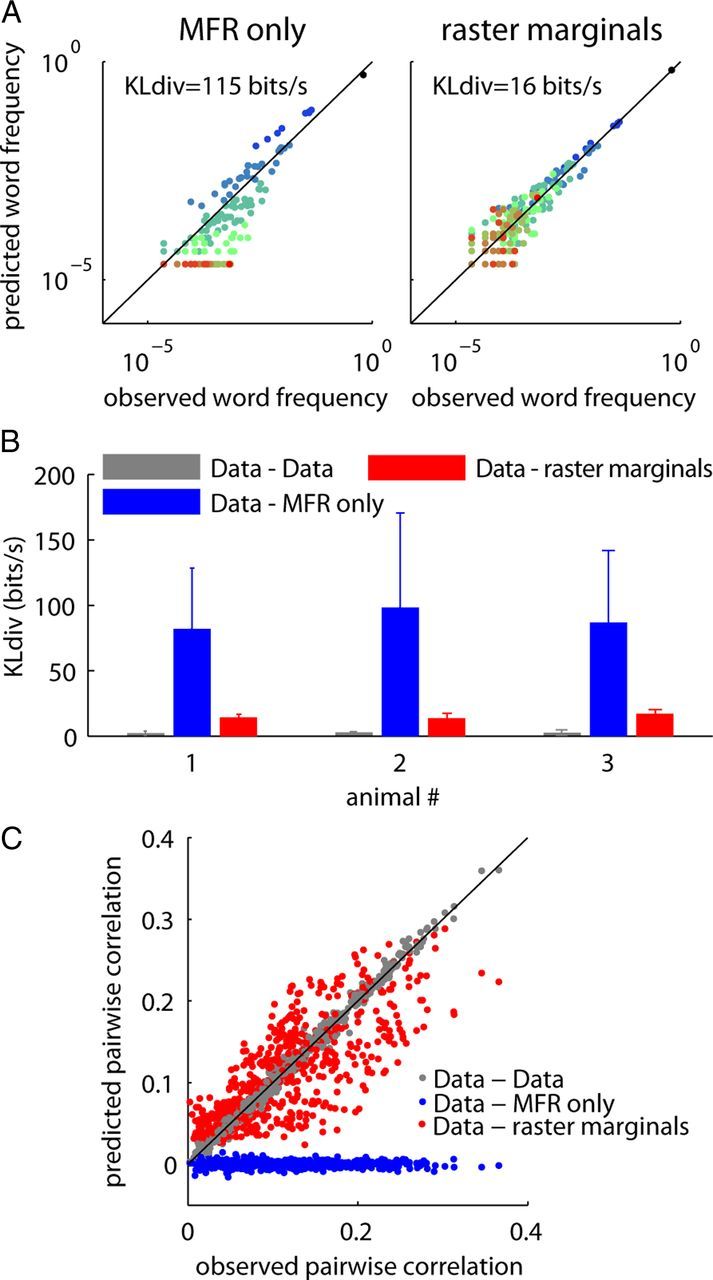
The raster marginals model accounts for the word distribution observations in rat A1. A, Fit between the MFR and raster marginals models to the word distribution in epoch S2 of Figure 1C. B, Summary data for the fit of the MFR and raster marginals models to the word distributions in the eight conditions in each animal (six in one of the rats). The bars represent the mean KLdiv. Error bars indicate SD. The gray bars indicate the KLdiv between two halves of the experimental data. C, The fit of the MFR and raster marginals models for the pairwise correlations (across all the conditions and animals). The gray points show how well the pairwise correlation measurement from one half of the experimental data describes the second half.

Although the raster marginals model greatly outperforms prediction from MFRs, it still does not provide a perfect fit to the observed word distributions (Fig. 3B, red vs gray). To gain an intuition for the quality of the fit, we examined how well the model predicted specific pairwise correlations. Figure 3C shows the correlation between each pair of spike trains in the original data plotted against the correlation predicted by the raster marginals model. The spread of the points around the diagonal indicates the extent to which factors beyond population dynamics affect pairwise correlations.

Nonetheless, the raster marginals model was sufficient to predict the observed KLdiv between pairs of word distributions. Indeed, the KLdiv measured from the synthetic rasters produced by the raster marginals model closely matched the KLdiv measured from the original data, recapitulating all the effects of cortical state and stimulus presence that we had observed in the actual data (Fig. 4A,B). To put the model to a further test, we computed the KLdiv between pairs of word distributions in which one was observed while the other was synthetic. These KLdiv values were also found to be close to the corresponding values of KLdiv between pairs of the original word distributions (Fig. 4C), with a small additive offset approximately equal to the residual distance between the original and model data (compare Fig. 3B).

Figure 4.

KLdiv between word distributions in rat A1 is captured by the raster marginals model. A, The model successfully reproduces the KLdiv measurements in Figure 1F–H. B, D_s[P||Q], the actual KLdiv between word distributions, is plotted versus D_s[P̂||Q̂], the KLdiv predicted by the raster marginals model. The plot shows data from all pairs of word distributions in the three animals superimposed. The fact that the points fall on the diagonal indicates that the actual KLdiv (Fig. 1F–H) and predicted KLdiv (A) are very close. C, D_s[P||Q] versus D_s[P||Q̂]. D, D_s[P||Q] versus D_s[P̃||Q̃], the KLdiv predicted by MFR alone, indicating a poor fit.

The raster marginals model, however, could not be further simplified. For instance, producing uncorrelated random spike trains according to MFRs alone did not provide an accurate prediction (Fig. 4D). Thus, while a model based on firing rates alone is poor at predicting KLdiv between word distributions, population rate dynamics provides a good approximation of individual word distributions and can therefore accurately predict KLdiv between pairs of distributions.

The raster marginals model accounts for distributions of firing patterns in cat V1

To further test the validity of the raster marginals model, we asked if it can also account for the firing patterns of neurons in the visual cortex. We analyzed a set of acute recordings from cat V1 made with a 96-channel multi-electrode array (Benucci et al., 2009; Busse et al., 2009). Every experiment lasted for many hours, during which blocks of specific visual stimuli were presented, including drifting and flashing gratings, plaids, random bars, natural movies, and others. In total, we analyzed data from 64 blocks of data (each lasting 14–50 min) from nine animals, yielding 200 pairs of blocks in which word distributions could be compared. For each animal we selected a random subset of 16 of the 96 electrodes, and compared the word distributions in the different blocks across these electrodes. This procedure was repeated five times, producing a total of 1000 comparisons.

In these recordings, the stimulus presentation did make a difference in terms of word distributions. We compared the activity measured during spontaneous activity with those measured during responses to gratings and natural movies (Fig. 5A). Similarly to earlier results in ferret V1 (Berkes et al., 2011), we found that spontaneous word distributions were more similar to those of natural movies than to gratings (Fig. 5B).

Figure 5.

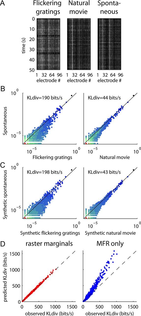
KLdiv between word distributions in cat V1 is captured by the raster marginals model. A, Example rasters from three blocks with different kinds of stimuli. B, Comparison of the word distributions during spontaneous activity with gratings and natural movies in cat V1. C, Comparison of word distributions generated by the raster marginals model using parameters derived from the same three conditions. Note the close match to the plots in B. D, Observed KLdiv for each pair of blocks versus KLdiv predicted by the raster marginals model (red) and the MFRs alone (blue), for data from nine cats. As with rat data, the raster marginals model provides an accurate prediction while MFR alone does not.

However, this dependence of word distribution on stimulus type was fully explained by the raster marginals model (Fig. 5C). In fact, the model accurately predicted the measured KLdiv across all pairs of stimuli in the dataset, not just gratings and natural movies (Fig. 5D). The success of the raster marginals model in explaining this large body of data indicates that here, as in the data from rat A1 discussed earlier, word distributions primarily reflect changes in population rate dynamics, rather than interactions between individual spike trains.

Statistical properties of the PRd

The success of the raster marginals model suggests that to understand word distributions, it is desirable to have a succinct model of the PRd. We found that a lognormal distribution, with a further shift to allow for bins of zero firing rate (see Materials and Methods), provided an accurate fit to the PRd measured in cat V1 experiments (Fig. 6A). To quantify the quality of the fit, we computed for each block the KLdiv between the shifted lognormal fit and the actual PRd (see Materials and Methods). In eight of the nine animals, we found a good fit between the two in most of the blocks (Fig. 6B).

Figure 6.

Statistical properties of the PRd. A, Example of a shifted lognormal fit to PRd of activity in one block from cat V1 dataset. In this particular example the KLdiv between the actual PRd and the fit is 20 bits/s. B, The KLdiv between the shifted lognormal fit and the observed PRd for each one of the blocks. Circles indicate the median KLdiv for each animal. In eight of the nine animals PRd is well described by a shifted lognormal distribution. C, KLdiv of word distributions is bounded from below by KLdiv of PRds. The panel shows the relationship of the KLdiv between word distributions of different blocks and the KLdiv between the corresponding PRds. As in Figure 5D, we use the 200 available pairs of blocks, with five different (random) selections of 16 of the 96 electrodes, for a total of 1000 points. Note that all points are to the right of the equality line, indicating a strict lower bound.

One of the mathematical motivations for the raster marginals model is the decomposition of the KLdiv into two parts, one of which depends only on the PRd. In more detail, let P(w) and Q(w) be two distributions of N-bit words w (for example with P representing the word distribution for spontaneous activity and Q that evoked by a particular sensory stimulus). Let r = r(w) denote the total number of spikes (i.e., 1s) in a word w. Since r is fully determined by w, it holds that

The second equality is known as the chain rule for relative entropy (Cover and Thomas, 1991). Equation 1 implies that the KLdiv is a sum of a component determined solely by the population rate dynamics (i.e., the PRd) and of a component determined by differences in the firing patterns across similar levels of population activation in P(w) and Q(w). Equation 1 has several additional implications, one of which is that D[P(r)||Q(r)] is a lower bound on D[P(w)||Q(w)]. Figure 6C shows the relationship between the (symmetrized) KLdiv of the full word distribution for blocks of cat data, and the (symmetrized) KLdiv of the PRds. As predicted, the KLdiv of the PRds forms a lower bound for the KLdiv of the full word distribution. However, the poor match seen in Figure 6C also indicates a significant contribution of the conditional KLdiv (the last term in Eq. 1). The fact that the raster marginals model makes a good prediction of KLdiv implies that it accurately approximates this conditional KLdiv term.

Explaining the apparent effect of development on word distributions

Cortical dynamics changes markedly over development: the juvenile visual cortex exhibits a state of primarily silent activity punctuated by occasional large population bursts that changes by adulthood into a more continuous pattern (Colonnese et al., 2010). These changes in cortical dynamics occur even in dark-reared animals (Golshani et al., 2009; Rochefort et al., 2009), so they cannot reflect learning of the visual environment. Could changes in cortical dynamics explain the developmental increase in similarity between spontaneous and evoked word distributions reported in ferrets by Berkes et al. (2011) (Fig. 7A)?

To answer this question, we used the raster marginals model to construct synthetic word distributions using parameters derived from previously published reports. According to Fiser et al. (2004), mean V1 firing rates in juvenile ferrets during periods of ongoing and sensory-evoked activities were 20 and 40 spikes/s, while the corresponding values for adult ferrets were 60 and 75 spikes/s. We synthesized “spontaneous” and “evoked” activity by allocating each electrode's MFR according to a Gaussian distribution with these means, with a PRd sampled from a shifted lognormal distribution as in our own V1 data (Fig. 7B; see Materials and Methods). Similarly to the ferret data, KLdiv between synthetic “juvenile” word distributions was several times higher than in synthetic “adult” data (Fig. 7C,D). As in the ferret data, comparison with synthetic trains computed from MFRs alone confirmed that these differences did not simply reflect changes in firing rates, but changes in correlation; however, the success of the raster marginals model indicated that these correlations could again be explained by population rate dynamics (Fig. 7D, bottom).

Word distributions in a randomly connected network

The above analyses suggest that changes in cortical dynamics, rather than learning-related synaptic plasticity, underlie the increased match of spontaneous to evoked word distributions in adult animals. But what could cause these changed dynamics? In adult animals, changes in cortical dynamics are believed to reflect changes in neuromodulatory and tonic glutamatergic drive (Harris and Thiele, 2011); across development, changes in cellular conductances (Kasper et al., 1994; Etherington and Williams, 2011; Guan et al., 2011) could also contribute to changed dynamics.

To demonstrate how such changes could alter word distributions even without synaptic weight modifications, we analyzed the joint structure of 16 multiunit spike trains in a simulated network of randomly connected neurons (Fig. 8A). As usual, we compared multineuron word distributions measured during spontaneous activity with those measured during driven activity. To mimic sensory stimulation, this driven activity was obtained by providing the network with an external spatiotemporally structured input (see Materials and Methods).

Figure 8.

Spontaneous and input-driven word distributions in a randomly connected recurrent spiking network can shift from a mismatch to a match upon change in intrinsic properties of the network. A, Schematic of the network, containing 80% excitatory and 20% inhibitory neurons. B, In condition 1, background depolarization is weak and firing adaptation of the excitatory neurons is strong. In this condition, the spontaneous and evoked word distributions produced by the network substantially differ. C, In condition 2, background depolarization is strong and adaptation weak. In this condition, spontaneous and evoked word distributions are similar. D, Same analysis as in Figure 7A,D (bottom) for spiking network data (S, spontaneous; Id, input driven). E, PRd for spontaneous (left) and external input driven (right) conditions in the spiking network. Note that the PRds for spontaneous and evoked activity differ greatly for condition 1, but not for condition 2. F, Same analysis as in Figure 3B for spiking network data. Error bars indicate SDs over the four conditions in which we examined the network dynamics (spontaneous and input-driven, in conditions 1 and 2).

With a fixed synaptic weight matrix, we simulated two conditions: one in which neurons exhibited strong cellular spike-frequency adaptation and received little background depolarization, and a second condition of weak adaptation and high background rate. As shown in previous computational models (Compte et al., 2003; Hill and Tononi, 2005; Holcman and Tsodyks, 2006; Destexhe, 2009), the first condition produced slow global fluctuations in activity, alternating spontaneously between active periods where recurrent excitation causes self-sustaining activity (“up states”), and silent periods that occur after sufficient adaptation has occurred to prevent their continuation (“down states”). Conversely, the second condition provided a state of more constant population activity.

The results obtained with this fixed artificial network recapitulated the main findings obtained with actual recordings: a change in the dynamics of population firing rate determined the match or mismatch between the word distributions seen in spontaneous and evoked activity. Indeed, while a mismatch between the spontaneous and evoked word distributions was found in the first condition (Fig. 8B), a close match was observed in the second (Fig. 8C).

To investigate the role of correlations in producing the KLdivs observed in these simulations, we again computed the KLdiv between word distributions of the original data and of synthetic rasters obtained using only the MFRs (Fig. 8D). As with the ferret data and raster marginals model (Fig. 7), differences between the original data and MFR-only model indicate the presence of correlations in the network, which became more pronounced in the second condition. The distinct KLdiv measures within conditions (e.g., gray vs pink bars) are qualitatively different from Figure 7, likely reflecting a difference in the shape of the PRds produced by the network, when compared with V1 (compare Figs. 8E, 6A). Finally, we note that the raster marginals model provided an accurate approximation for the structure of word distributions produced by the network (Fig. 8F) and for the KLdiv between pairs of word distributions in the different conditions (data not shown). We conclude that changes in the dynamical state of even a randomly connected network can cause a change from low to high match between spontaneous and evoked activity, without any form of synaptic plasticity.

Discussion

We assessed similarities and differences between probability distributions of cortical population activity using the KLdiv between multiunit word distributions. KLdiv depended on both cortical state and sensory stimuli. Changes in MFRs were not sufficient to predict the KLdiv between observed word distributions, indicating that correlations also contributed substantially. Nevertheless, the experimentally measured KLdiv could be accurately predicted by the raster marginals model, in which all correlations resulted from population rate dynamics, rather than precise interactions between cells. A simulated spiking network model of fixed random connectivity could exhibit either similarity or difference between spontaneous and sensory-evoked word distributions, according to its cellular parameters. We conclude that similarities and differences in KLdiv between multiunit word distributions can primarily reflect changes in population dynamics, rather than the precise interactions between spike trains that would be a hallmark of learning.

The raster marginals model

It is important to distinguish the raster marginals model from the maximum entropy models typically used to describe the word distribution structure (Schneidman et al., 2006; Shlens et al., 2006; Yu et al., 2008; Roudi et al., 2009; Ohiorhenuan et al., 2010; Ganmor et al., 2011a, b; Yu et al., 2011). In the latter, a distribution is fit that matches specific pairwise or higher order correlations, usually requiring at least an order of N² parameters for a population of N neurons. In the raster marginals model, however, correlations are only produced as a result of population rate dynamics as measured by the summed rate of all neurons, and the temporal structure of the spike trains is discarded. The simplicity of the model is reflected by the fact that it uses only 2N parameters.

Because of its simplicity, we do not expect the model to provide an entirely accurate description of multiunit word distributions: indeed, the match between the word distributions of the model and original data, while significantly better than for distributions produced by MFRs alone, was not perfect (Figs. 3B,C 8F). Nevertheless, the ability of this simple model to accurately predict the KLdiv between experimental conditions (Figs. 4B, 5D) indicates that KLdiv is dominated by changes in population dynamics as parameterized by the model. Therefore, the raster marginals model may provide a useful tool to disentangle genuine higher order interactions from correlations induced by population rate dynamics.

Sampling-based representation and learning

Theoretical support for the sampling-based representation hypothesis comes from a class of artificial neural network models (“generative networks”), which produce such a behavior (Ackley et al., 1985; Dayan et al., 1995; Hinton and Salakhutdinov, 2006; Buesing et al., 2011; Pecevski et al., 2011). A recent analysis of recordings from ferret visual cortex over the course of development found a gradual decrease in the KLdiv between the word distribution of spontaneous and evoked activity, as would be seen across training of a generative network. Moreover, the spontaneous word distribution in adult ferret V1 was similar to the distribution during the presentation of natural movies, which presumably shared statistical structure with the animal's previous experience, but not of artificial drifting gratings (Berkes et al., 2011).

Here we provide a potentially more parsimonious explanation for these findings. We show that similar results can be obtained from the raster marginals model, suggesting that they are not evidence that a probabilistic model of the environment has been learned and encoded in synaptic weights, but rather of similar population rate dynamics in the two conditions (Figs. 5A–C, 7). Without replicating the experiments with animals of different ages we cannot altogether dismiss the possibility that population rate dynamics is not the explanation for the developmental changes reported in (Berkes et al., 2011). However, if population dynamics does not account for these findings, one has to conclude that neural population dynamics in ferret V1 and in the data analyzed here differs in some profound manner. This would be an important and unexpected finding that would require further investigation.

Our results demonstrate that in auditory and visual cortices as well as simulated recurrent networks, word distributions reflect not only on the interaction of external inputs with the synaptic weight matrix, but also dynamical properties of the networks. Such dynamical properties can change rapidly and reversibly with cortical state (Fig. 1C–E), and be caused by changes in properties such as cellular adaptation and background input (Fig. 8), which are in turn controlled by neuromodulatory tone and tonic glutamatergic input (Harris and Thiele, 2011; Poulet et al., 2012), as well as changing over development (Kasper et al., 1994; Etherington and Williams, 2011; Guan et al., 2011).

Convincingly demonstrating that learning has occurred by comparing word distributions is difficult for a number of reasons. First, as the current work shows, word distribution structure is dominated by population dynamics, whereas learning would be expected to primarily manifest itself as a change in firing statistics of specific subgroups of neurons. Therefore, to unveil the effect of learning, it is necessary to quantify the specific pairwise and higher order interactions between spike trains, beyond those induced by fluctuations in population rate. Whereas several computational approaches for doing so exist (one of them being to measure deviations between observed pairwise correlations and those predicted from population rate; Fig. 3C), there is no reason to think that any one of them is of particular biological significance. The real challenge, however, is not in measuring the specific interactions, but in showing that their change across conditions is due to learning, rather than other processes. To demonstrate this point, we have presented several different examples of processes, which are not learning-related but have a profound effect on the structure of word distribution. In summary, the level of similarity between spontaneous and evoked activity must be interpreted with caution: its changes need not be a signature of learning-related modifications in synaptic strength; and high similarity does not imply that a network has learned a model of the environment.

Notes

MATLAB implementation of the raster marginals model is available at http://www.carandinilab.net/code/RasterMarginals.zip. This material has not been peer reviewed.

References

- Ackley DH, Hinton GE, Sejnowski TJ. A learning algorithm for Boltzmann machines. Cogn Sci. 1985;9:147–169. [Google Scholar]
- Amari S, Nakahara H, Wu S, Sakai Y. Synchronous firing and higher-order interactions in neuron pool. Neural Comput. 2003;15:127–142. doi: 10.1162/089976603321043720. [DOI] [PubMed] [Google Scholar]
- Benucci A, Ringach DL, Carandini M. Coding of stimulus sequences by population responses in visual cortex. Nat Neurosci. 2009;12:1317–1324. doi: 10.1038/nn.2398. [DOI] [PMC free article] [PubMed] [Google Scholar]
- Berkes P, Orbán G, Lengyel M, Fiser J. Spontaneous cortical activity reveals hallmarks of an optimal internal model of the environment. Science. 2011;331:83–87. doi: 10.1126/science.1195870. [DOI] [PMC free article] [PubMed] [Google Scholar]
- Brette R, Gerstner W. Adaptive exponential integrate-and-fire model as an effective description of neuronal activity. J Neurophysiol. 2005;94:3637–3642. doi: 10.1152/jn.00686.2005. [DOI] [PubMed] [Google Scholar]
- Brualdi RA. Algorithms for constructing (0,1)-matrices with prescribed row and column sum vectors. Discrete Math. 2006;306:3054–3062. [Google Scholar]
- Buesing L, Bill J, Nessler B, Maass W. Neural dynamics as sampling: a model for stochastic computation in recurrent networks of spiking neurons. PLoS Comput Biol. 2011;7:e1002211. doi: 10.1371/journal.pcbi.1002211. [DOI] [PMC free article] [PubMed] [Google Scholar]
- Busse L, Wade AR, Carandini M. Representation of concurrent stimuli by population activity in visual cortex. Neuron. 2009;64:931–942. doi: 10.1016/j.neuron.2009.11.004. [DOI] [PMC free article] [PubMed] [Google Scholar]
- Clement EA, Richard A, Thwaites M, Ailon J, Peters S, Dickson CT. Cyclic and sleep-like spontaneous alternations of brain state under urethane anaesthesia. PLoS One. 2008;3:e2004. doi: 10.1371/journal.pone.0002004. [DOI] [PMC free article] [PubMed] [Google Scholar]
- Colonnese MT, Kaminska A, Minlebaev M, Milh M, Bloem B, Lescure S, Moriette G, Chiron C, Ben-Ari Y, Khazipov R. A conserved switch in sensory processing prepares developing neocortex for vision. Neuron. 2010;67:480–498. doi: 10.1016/j.neuron.2010.07.015. [DOI] [PMC free article] [PubMed] [Google Scholar]
- Compte A, Sanchez-Vives MV, McCormick DA, Wang XJ. Cellular and network mechanisms of slow oscillatory activity (<1 Hz) and wave propagations in a cortical network model. J Neurophysiol. 2003;89:2707–2725. doi: 10.1152/jn.00845.2002. [DOI] [PubMed] [Google Scholar]
- Cover TM, Thomas JA. Elements of information theory. New York: Wiley; 1991. [Google Scholar]
- Curto C, Sakata S, Marguet S, Itskov V, Harris KD. A simple model of cortical dynamics explains variability and state dependence of sensory responses in urethane-anesthetized auditory cortex. J Neurosci. 2009;29:10600–10612. doi: 10.1523/JNEUROSCI.2053-09.2009. [DOI] [PMC free article] [PubMed] [Google Scholar]
- Davison AP, Brüderle D, Eppler J, Kremkow J, Muller E, Pecevski D, Perrinet L, Yger P. PyNN: a common interface for neuronal network simulators. Front Neuroinform. 2008;2:11. doi: 10.3389/neuro.11.011.2008. [DOI] [PMC free article] [PubMed] [Google Scholar]
- Dayan P, Hinton GE, Neal RM, Zemel RS. The Helmholtz machine. Neural computation. 1995;7:889–904. doi: 10.1162/neco.1995.7.5.889. [DOI] [PubMed] [Google Scholar]
- Destexhe A. Self-sustained asynchronous irregular states and Up-Down states in thalamic, cortical and thalamocortical networks of nonlinear integrate-and-fire neurons. J Comput Neurosci. 2009;27:493–506. doi: 10.1007/s10827-009-0164-4. [DOI] [PubMed] [Google Scholar]
- DeWeese MR, Zador AM. Non-Gaussian membrane potential dynamics imply sparse, synchronous activity in auditory cortex. J Neurosci. 2006;26:12206–12218. doi: 10.1523/JNEUROSCI.2813-06.2006. [DOI] [PMC free article] [PubMed] [Google Scholar]
- Ernst MO, Banks MS. Humans integrate visual and haptic information in a statistically optimal fashion. Nature. 2002;415:429–433. doi: 10.1038/415429a. [DOI] [PubMed] [Google Scholar]
- Etherington SJ, Williams SR. Postnatal development of intrinsic and synaptic properties transforms signaling in the layer 5 excitatory neural network of the visual cortex. J Neurosci. 2011;31:9526–9537. doi: 10.1523/JNEUROSCI.0458-11.2011. [DOI] [PMC free article] [PubMed] [Google Scholar]
- Fiser J, Chiu C, Weliky M. Small modulation of ongoing cortical dynamics by sensory input during natural vision. Nature. 2004;431:573–578. doi: 10.1038/nature02907. [DOI] [PubMed] [Google Scholar]
- Fiser J, Berkes P, Orbán G, Lengyel M. Statistically optimal perception and learning: from behavior to neural representations. Trends Cogn Sci. 2010;14:119–130. doi: 10.1016/j.tics.2010.01.003. [DOI] [PMC free article] [PubMed] [Google Scholar]
- Franklin DW, Wolpert DM. Computational mechanisms of sensorimotor control. Neuron. 2011;72:425–442. doi: 10.1016/j.neuron.2011.10.006. [DOI] [PubMed] [Google Scholar]
- Ganmor E, Segev R, Schneidman E. Sparse low-order interaction network underlies a highly correlated and learnable neural population code. Proc Natl Acad Sci U S A. 2011a;108:9679–9684. doi: 10.1073/pnas.1019641108. [DOI] [PMC free article] [PubMed] [Google Scholar]
- Ganmor E, Segev R, Schneidman E. The architecture of functional interaction networks in the retina. J Neurosci. 2011b;31:3044–3054. doi: 10.1523/JNEUROSCI.3682-10.2011. [DOI] [PMC free article] [PubMed] [Google Scholar]
- Gewaltig M-O, Diesmann M. NEST (NEural simulation tool) Scholarpedia. 2007;2:1430. [Google Scholar]
- Golshani P, Gonçalves JT, Khoshkhoo S, Mostany R, Smirnakis S, Portera-Cailliau C. Internally mediated developmental desynchronization of neocortical network activity. J Neurosci. 2009;29:10890–10899. doi: 10.1523/JNEUROSCI.2012-09.2009. [DOI] [PMC free article] [PubMed] [Google Scholar]
- Grün S. Data-driven significance estimation for precise spike correlation. J Neurophysiol. 2009;101:1126–1140. doi: 10.1152/jn.00093.2008. [DOI] [PMC free article] [PubMed] [Google Scholar]
- Guan D, Horton LR, Armstrong WE, Foehring RC. Postnatal development of A-type and Kv1- and Kv2-mediated potassium channel currents in neocortical pyramidal neurons. J Neurophysiol. 2011;105:2976–2988. doi: 10.1152/jn.00758.2010. [DOI] [PMC free article] [PubMed] [Google Scholar]
- Harris KD, Thiele A. Cortical state and attention. Nat Rev Neurosci. 2011;12:509–523. doi: 10.1038/nrn3084. [DOI] [PMC free article] [PubMed] [Google Scholar]
- Hazan L, Zugaro M, Buzsáki G. Klusters, NeuroScope, NDManager: a free software suite for neurophysiological data processing and visualization. J Neurosci Methods. 2006;155:207–216. doi: 10.1016/j.jneumeth.2006.01.017. [DOI] [PubMed] [Google Scholar]
- Hill S, Tononi G. Modeling sleep and wakefulness in the thalamocortical system. J Neurophysiol. 2005;93:1671–1698. doi: 10.1152/jn.00915.2004. [DOI] [PubMed] [Google Scholar]
- Hinton GE, Salakhutdinov RR. Reducing the dimensionality of data with neural networks. Science. 2006;313:504–507. doi: 10.1126/science.1127647. [DOI] [PubMed] [Google Scholar]
- Holcman D, Tsodyks M. The emergence of Up and Down states in cortical networks. PLoS Comput Biol. 2006;2:e23. doi: 10.1371/journal.pcbi.0020023. [DOI] [PMC free article] [PubMed] [Google Scholar]
- Hoyer PO, Hyvarinen A. Interpreting neural response variability as Monte Carlo sampling of the posterior. In: Becker S, et al., editors. Advances in neural information processing systems. Cambridge, MA: MIT; 2003. pp. 277–284. [Google Scholar]
- Kasper EM, Larkman AU, Lübke J, Blakemore C. Pyramidal neurons in layer-5 of the rat visual-cortex. 2. Development of electrophysiological properties. J Comp Neurol. 1994;339:475–494. doi: 10.1002/cne.903390403. [DOI] [PubMed] [Google Scholar]
- Kenet T, Bibitchkov D, Tsodyks M, Grinvald A, Arieli A. Spontaneously emerging cortical representations of visual attributes. Nature. 2003;425:954–956. doi: 10.1038/nature02078. [DOI] [PubMed] [Google Scholar]
- Kersten D, Mamassian P, Yuille A. Object perception as Bayesian inference. Annu Rev Psychol. 2004;55:271–304. doi: 10.1146/annurev.psych.55.090902.142005. [DOI] [PubMed] [Google Scholar]
- Knill DC, Richards W. Perception as bayesian inference. New York: Cambridge UP; 1996. [Google Scholar]
- Luczak A, Barth ó P, Marguet SL, Buzsáki G, Harris KD. Sequential structure of neocortical spontaneous activity in vivo. Proc Natl Acad Sci U S A. 2007;104:347–352. doi: 10.1073/pnas.0605643104. [DOI] [PMC free article] [PubMed] [Google Scholar]
- Luczak A, Barth ó P, Harris KD. Spontaneous events outline the realm of possible sensory responses in neocortical populations. Neuron. 2009;62:413–425. doi: 10.1016/j.neuron.2009.03.014. [DOI] [PMC free article] [PubMed] [Google Scholar]
- Macke JH, Opper M, Bethge M. Common input explains higher-order correlations and entropy in a simple model of neural population activity. Phys Rev Lett. 2011;106:208102. doi: 10.1103/PhysRevLett.106.208102. [DOI] [PubMed] [Google Scholar]
- Marguet SL, Harris KD. State-dependent representation of amplitude-modulated noise stimuli in rat auditory cortex. J Neurosci. 2011;31:6414–6420. doi: 10.1523/JNEUROSCI.5773-10.2011. [DOI] [PMC free article] [PubMed] [Google Scholar]
- Moreno-Bote R, Knill DC, Pouget A. Bayesian sampling in visual perception. Proc Natl Acad Sci U S A. 2011;108:12491–12496. doi: 10.1073/pnas.1101430108. [DOI] [PMC free article] [PubMed] [Google Scholar]
- Ohiorhenuan IE, Mechler F, Purpura KP, Schmid AM, Hu Q, Victor JD. Sparse coding and high-order correlations in fine-scale cortical networks. Nature. 2010;466:617–621. doi: 10.1038/nature09178. [DOI] [PMC free article] [PubMed] [Google Scholar]
- Okun M, Lampl I. Instantaneous correlation of excitation and inhibition during ongoing and sensory-evoked activities. Nat Neurosci. 2008;11:535–537. doi: 10.1038/nn.2105. [DOI] [PubMed] [Google Scholar]
- Okun M, Naim A, Lampl I. The subthreshold relation between cortical local field potential and neuronal firing unveiled by intracellular recordings in awake rats. J Neurosci. 2010;30:4440–4448. doi: 10.1523/JNEUROSCI.5062-09.2010. [DOI] [PMC free article] [PubMed] [Google Scholar]
- Pecevski D, Buesing L, Maass W. Probabilistic inference in general graphical models through sampling in stochastic networks of spiking neurons. PLoS Comput Biol. 2011;7:e1002294. doi: 10.1371/journal.pcbi.1002294. [DOI] [PMC free article] [PubMed] [Google Scholar]
- Pillow JW, Shlens J, Paninski L, Sher A, Litke AM, Chichilnisky EJ, Simoncelli EP. Spatio-temporal correlations and visual signalling in a complete neuronal population. Nature. 2008;454:995–999. doi: 10.1038/nature07140. [DOI] [PMC free article] [PubMed] [Google Scholar]
- Poulet JF, Petersen CC. Internal brain state regulates membrane potential synchrony in barrel cortex of behaving mice. Nature. 2008;454:881–885. doi: 10.1038/nature07150. [DOI] [PubMed] [Google Scholar]
- Poulet JF, Fernandez LM, Crochet S, Petersen CC. Thalamic control of cortical states. Nat Neurosci. 2012;15:370–372. doi: 10.1038/nn.3035. [DOI] [PubMed] [Google Scholar]
- Rao AR, Jana R, Bandyopadhyay S. A Markov Chain Monte Carlo Method for generating random (0, 1)-matrices with given marginals. Sankhya Series A. 1996;58:225–242. [Google Scholar]
- Rao RPN, Olshausen BA, Lewicki MS. Probabilistic models of the brain: perception and neural function. In: Rajesh PN, Rao B, Olshausen A, Lewicki MS, editors. Cambridge, MA: MIT; 2002. [Google Scholar]
- Renart A, de la Rocha J, Bartho P, Hollender L, Parga N, Reyes A, Harris KD. The asynchronous state in cortical circuits. Science. 2010;327:587–590. doi: 10.1126/science.1179850. [DOI] [PMC free article] [PubMed] [Google Scholar]
- Ringach DL. Spontaneous and driven cortical activity: implications for computation. Curr Opin Neurobiol. 2009;19:439–444. doi: 10.1016/j.conb.2009.07.005. [DOI] [PMC free article] [PubMed] [Google Scholar]
- Rochefort NL, Garaschuk O, Milos RI, Narushima M, Marandi N, Pichler B, Kovalchuk Y, Konnerth A. Sparsification of neuronal activity in the visual cortex at eye-opening. Proc Natl Acad Sci U S A. 2009;106:15049–15054. doi: 10.1073/pnas.0907660106. [DOI] [PMC free article] [PubMed] [Google Scholar]
- Roudi Y, Nirenberg S, Latham PE. Pairwise maximum entropy models for studying large biological systems: when they can work and when they can't. PLoS Comput Biol. 2009;5:e1000380. doi: 10.1371/journal.pcbi.1000380. [DOI] [PMC free article] [PubMed] [Google Scholar]
- Ryser HJ. Combinatorial properties of matrices of zeros and ones. Canad J Math. 1957;9:371–377. [Google Scholar]
- Ryser HJ. Matrices of zeros and ones. Bull Am Math Soc. 1960;66:442–464. [Google Scholar]
- Schneidman E, Berry MJ, 2nd, Segev R, Bialek W. Weak pairwise correlations imply strongly correlated network states in a neural population. Nature. 2006;440:1007–1012. doi: 10.1038/nature04701. [DOI] [PMC free article] [PubMed] [Google Scholar]
- Shlens J, Field GD, Gauthier JL, Grivich MI, Petrusca D, Sher A, Litke AM, Chichilnisky EJ. The structure of multi-neuron firing patterns in primate retina. J Neurosci. 2006;26:8254–8266. doi: 10.1523/JNEUROSCI.1282-06.2006. [DOI] [PMC free article] [PubMed] [Google Scholar]
- Strong SP, Koberle R, van Steveninck RRD, Bialek W. Entropy and information in neural spike trains. Phys Rev Lett. 1998;80:197–200. [Google Scholar]
- Tkacik G, Prentice JS, Balasubramanian V, Schneidman E. Optimal population coding by noisy spiking neurons. Proc Natl Acad Sci U S A. 2010;107:14419–14424. doi: 10.1073/pnas.1004906107. [DOI] [PMC free article] [PubMed] [Google Scholar]
- Yu S, Huang D, Singer W, Nikolic D. A small world of neuronal synchrony. Cereb Cortex. 2008;18:2891–2901. doi: 10.1093/cercor/bhn047. [DOI] [PMC free article] [PubMed] [Google Scholar]
- Yu S, Yang H, Nakahara H, Santos GS, Nikolić D, Plenz D. Higher-order interactions characterized in cortical activity. J Neurosci. 2011;31:17514–17526. doi: 10.1523/JNEUROSCI.3127-11.2011. [DOI] [PMC free article] [PubMed] [Google Scholar]