Metal artefact reduction with cone beam CT: an in vitro study

Abstract

Background

Metal in a patient's mouth has been shown to cause artefacts that can interfere with the diagnostic quality of cone beam CT. Recently, a manufacturer has made an algorithm and software available which reduces metal streak artefact (Picasso Master 3D® machine; Vatech, Hwaseong, Republic of Korea).

Objectives

The purpose of this investigation was to determine whether or not the metal artefact reduction algorithm was effective and enhanced the contrast-to-noise ratio.

Methods

A phantom was constructed incorporating three metallic beads and three epoxy resin-based bone substitutes to simulate bone next to metal. The phantom was placed in the centre of the field of view and at the periphery. 10 data sets were acquired at 50–90 kVp. The images obtained were analysed using a public domain software ImageJ (NIH Image, Bethesda, MD). Profile lines were used to evaluate grey level changes and area histograms were used to evaluate contrast. The contrast-to-noise ratio was calculated.

Results

The metal artefact reduction option reduced grey value variation and increased the contrast-to-noise ratio. The grey value varied least when the phantom was in the middle of the volume and the metal artefact reduction was activated. The image quality improved as the peak kilovoltage increased.

Conclusion

Better images of a phantom were obtained when the metal artefact reduction algorithm was used.

Introduction

Cone beam CT (CBCT) was introduced as one of the most accurate imaging modalities for dental diagnostic purposes^1-2 and as an alternative to CT in diagnosing pathologies or dysfunctions of the craniomaxillofacial complex.^3-4 CBCT utilizes a cone beam-shaped X-ray source and acquires and reconstructs a whole volume of the head and neck area. The radiation dose required for CBCT is lower than that of CT if we consider images made for the same purposes.^5-6 Metal has been shown to cause artefacts that interfere with the diagnostic quality of CT and CBCT images.⁷ The examination of metal bodies shows strong beam hardening and scattering effect artefacts which lead to unsuitable images for diagnostic purposes.⁸ Tissues through which X-rays pass to form dental images alter the energy spectrum of the beam; metallic objects are known to alter that energy the most.⁹ Metal artefacts detected by CBCT influence the image quality by reducing the contrast, obscuring structures and impairing the detection of areas of interest, thereby making the diagnosis difficult and time-consuming.^10,11 Various methods for metal artefact reduction (MAR) on CBCT have been proposed. In some studies, new algorithms were proposed and used to improve image quality through enhancing the reconstruction of the image.¹² In other studies, the effect of increasing the radiation dose was examined by increasing either the milliampere second factor or the peak kilovoltage.^11-13 Many post-processing techniques for MAR also have been proposed.^12-15 In these studies, the amounts of metal artefact was assessed visually. The Picasso Master 3D® machine (Vatech, Hwaseong, Republic of Korea) has the option of applying an algorithm to decrease the metal artefact. Additionally, the same machine offers three volume sizes, two resolutions for each volume size and two quality levels for each resolution, which leads us to twelve different possibilities from which the operator may choose when acquiring data. The objective of this study was to investigate if the Picasso Master 3D machine reduces the metal artefact and increases the contrast-to-noise ratio (CNR) which will lead to a better image.

Experimental design and methods

The phantom used in this study consisted of a bucket, a square platform with three metallic beads, three epoxy resin-based bone substitutes (ERBSs)¹⁶ and a plastic rectangular box (Figure 1). The bucket was used to contain all of the parts. The plastic rectangular box was fixed to the bottom of the bucket with boxing wax on all its surfaces. On top of the box, the square platform was fixed with methylmethacrylate (one drop in each corner). The metallic beads were fixed on the square platform with polyurethane resin. The three beads represented the vertices of an equilateral triangle. Two of the ERBSs had a square shape and were fixed with methylmethacrylate over two sides of the equilateral triangle formed by the metallic beads. The third ERBS had a rectangular shape and was fixed with the same material outside of the triangle formed by the beads (Figure 2). The bucket was filled with water and placed on a platform connected to the CBCT machine. The platform was fixed to the machine with tape and the phantom was fixed to the platform with tape. Two series of ten images each were taken. For the first series the phantom was placed in the centre of the field. For the second series the phantom was moved to the periphery. Each series was divided into two groups of five CBCT volumes each: five were taken with the MAR and the other five without it. The current was fixed at 3.4 mA and five different peak kilovoltages were used: 90 kVp, 80 kVp, 70 kVp, 60 kVp and 50 kVp. The field of view was 16 × 7 cm, the voxel was size 0.2 and high-quality scans were acquired. In each volume the axial slice showing the ERBS and metallic beads was saved as a 24-bit (bitmap) image using the same monitor. The CBCT machine had a different setting for each image in each group. There was no digital manipulation done for the images. All of the images were collected using the same method by the same operator. A total of 20 images were collected—Figures 3 and 4 are examples of two images acquired. The images were evaluated according to three variables with public domain (free) image analysis software, ImageJ (NIH Image, Bethesda, MD; available from: rsb.info.nih.gov/ij/). Using the program, the area histograms were made for each slice. There were four areas per slice: the three ERBS areas and a water area, which served as a control. For each histogram, ImageJ calculated a mean and a standard deviation. After the profile lines were drawn, we computed the coordinates of the curve using ImageJ. The vertical axis (Y) values represent the grey value. Ymax–Ymin was calculated as the grey value variation for each line. For each peak kilovoltage, phantom location and MAR, the CNR was calculated as:

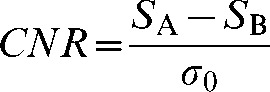Figure 1.

Phantom

Figure 2.

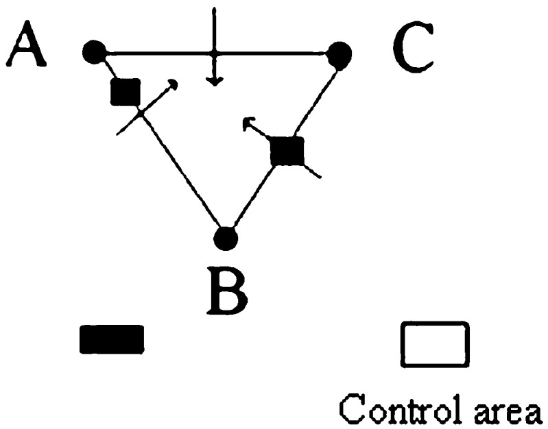
Points A, B and C represent the beads on the platform. The black rectangles represents the epoxy resin-based bone substitutes. The control area is represented by the white squre. The arrows represent where the profile lines were drawn. The area histograms were drawn over the four rectangles

Figure 3.

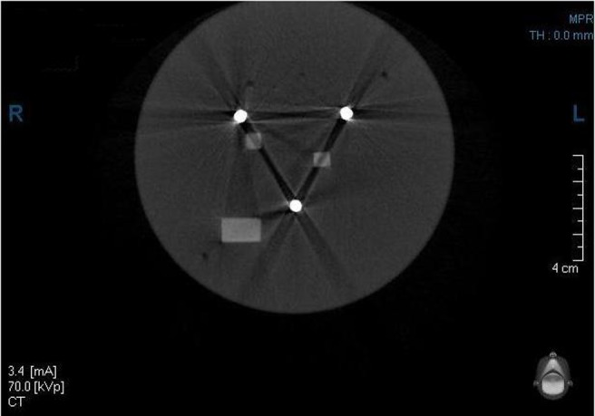
Image acquired at 70 kVp. The phantom placed in the central position. No metal artefact reduction was used

Figure 4.

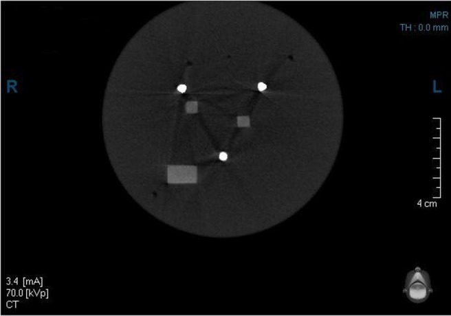
Image acquired at 70 kVp. The phantom was placed in the central position. The metal artefact reduction was used

where S_A is the mean of the area histogram of the rectangular ERBS, S_B is the mean for the area histogram of the control area and σ₀ is the standard deviation of the same control area.

Statistical methods

Data were analysed using multiple linear regression.¹⁷ A second-order model was used to investigate the effects of MAR (with or without), position (central or peripheral) and the linear trend in peak kilovoltage (50 kVp, 60 kVp, 70 kVp, 80 kVp and 90 kVp) on the three dependent variables: CNR, the grey value variation and area histogram's mean variation. Additionally, the two-factor interactions MAR by position, MAR by linear trend in peak kilovoltage and position by linear trend in peak kilovoltage as well as the quadratic trend (curvature) in peak kilovoltage were included in the statistical model. The regression equation we employed represented the peak kilovoltage level as deviations from the central value of 70 kVp and thus we present the average value (level) of the dependent variable at a peak kilovoltage of 70. Residual analyses indicated that the data were in reasonable conformity with the underlying assumptions of a normal distribution and constant variance and those terms higher than second order were not required. The squared multiple correlation coefficients (R²) indicated a good fit of this second-order model to the data. Profile lines and areas were analysed separately.

A final model for each dependent variable was selected using backward elimination.¹⁷ The effects of MAR and position were forced to be retained in the model. Interactions and curvature were retained only if p≤0.10; this choice of 0.10 was applied to prevent bias.¹⁷ For presentation of results, we show as a reference the regression equation for the peripheral position without MAR. Effects resulting from the use of MAR and central position are presented as deviations from the reference regression equation.

Results

Contrast-to-noise ratio

CNRs are given in Figure 5 and Table 1. The CNR at a peak kilovoltage of 70 was significantly higher (+7.12) with MAR than without MAR. Moreover, there was a steeper slope (+0.24) with MAR than without MAR. Also, the CNR was significantly higher in the central position (+3.44) than in the peripheral position.

Figure 5.

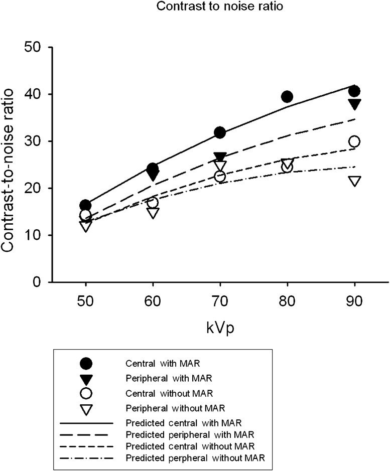
Observed and predicted contrast-to-noise ratios by metal artefact reduction (MAR&r par;) (with or without), position (central or peripheral) and peak kilovoltage

Table 1. Regression coefficients for relation of contrast-to-noise ratio to MAR, position and peak kilovoltage.

Reference (peripheral without MAR)		Regression coefficient (SE)
	Level (kVp=70)	19.03 (1.22) *
	Slope	0.34 (0.07) *
Factor	Effect
MAR	Change in level (kVp=70)	7.12 (1.41) *
	Change in slope	0.24 (0.10) ***
Central position	Change in level (kVp=70)	3.44 (1.41) ***
R2		0.89

MAR, metal artefact reduction; SE, standard error.

* p≤0.001.

** p≤0.01.

*** p≤0.05.

Grey level variation

Grey level variations are given in Figure 6 and Table 2. Grey level variation was significantly lower [changes in level of –26.63 for profile AB, –9.40 for profile BC, –43.80 for profile CA (Figure 2)] with MAR than without MAR for all three profiles. For profile CA, grey level variation was substantially lower (change of –11.90) in the peripheral position without MAR but was similar in the two positions with MAR [sum of –11.90 and 15.30, that is, a change of 3.40 (standard error =2.92, p=0.2632]. For all three profiles, the linear trend associated with peak kilovoltage had a less negative slope in the central position than in the peripheral position (changes in slope of +0.30 for profile AB, +0.39 for profile BC and +0.59 for profile CA).

Table 2. Regression coefficients for relation of grey level variation to MAR, position and peak kilovoltage.

		Regression coefficient (SE)
Reference (peripheral without MAR)		Profile AB	Profile BC	Profile CA
	Level (kVp=70)	47.61 (1.50) *	83.63 (2.09) *	64.40 (2.06) *
	Slope	−0.40 (0.09) *	−0.83 (0.12) *	−0.57 (0.10) *
Factor	Effect
MAR	Change in level (kVp=70)	−26.63 (1.73) *	−9.40 (2.41) **	−43.80 (2.92) *
Central position	Change in level (kVp=70)	−2.05 (1.73)	1.82 (2.41)	−11.90 (2.92) **
	Change in slope	0.30 (0.12) ***	0.39 (0.17) ***	0.59 (0.15) **
MAR and central position	Change in level (kVp=70)			15.30 (4.12) **
R2		0.95	0.84	0.96

MAR, metal artefact reduction; SE, standard error.

* p≤0.001.

** p≤0.01.

*** p≤0.05.

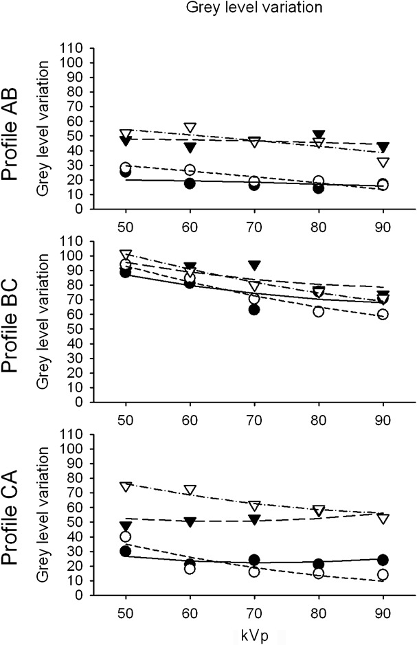
Observed and predicted grey level variation by metal artefact reduction (with or without), position (central or peripheral), profile (AB, BC or CA) and peak kilovoltage

Mean grey level

Mean grey levels are given in Figure 7 and Table 3. For all four areas, the mean grey level was significantly lower (changes in level of –6.43 for area AB, –7.82 for area BC, –13.12 for area control and –10.25 for area rectangle) with MAR than without MAR. The slope of the linear trend was less negative with MAR than without MAR (changes in slope of +0.56 for Area AB, +0.48 for Area BC, +0.49 for area control and +0.40 for area rectangle). For the control area, there was also a significant quadratic (curvature) trend in mean grey level associated with peak kilovoltage (p=0.0372).

Table 3. Regression coefficients for relation of mean grey level to MAR, position and peak kilovoltage.

		Regression coefficient (SE)
Reference (peripheral without MAR)		Area AB	Area BC	Area control	Area rectangle
	Level (kVp=70)	82.25 (1.68) *	86.99 (0.91) *	52.47 (0.29) *	102.32 (1.05) *
	Slope	−1.17 (0.08) *	−1.15 (0.05) *	−0.71 (0.01) *	−1.16 (0.06) *
	Curvature	0.0087 (0.0048)		0.0021 (0.0008) **
Factor	Effect
MAR	Change in level (kVp=70)	−6.43 (1.60) ***	−7.83 (1.05) *	−13.12 (0.27) *	−10.25 (1.21) *
	Change in slope	0.56 (0.11) *	0.48 (0.07) *	0.49 (0.02) *	0.40 (0.09) *
Central position	Change in level (kVp=70)	1.46 (1.60)	0.77 (1.05)	−0.90 (0.27) ***	1.85 (1.21)
R2		0.95	0.98	0.99	0.98

MAR, metal artefact reduction; SE, standard error.

* P≤0.001.

** P≤0.05.*** P≤0.01.

Observed and predicted mean grey level by metal artefact reduction (with or without), position (central or peripheral), area (AB, BC, control or rectangle) and peak kilovoltage

Discussion

Various methods have been proposed for MAR. The most obvious solution is to use materials such as titanium that cause fewer artefacts than other metals. The application of higher energy X-ray beams does not decrease the MAR, although the photon starvation effect may suggest this solution.¹⁸ Artificially generated projection data replace the eliminated data. Several approaches were described for data acquisition such as pattern recognition and linear or polynomial interpolation.^19-21 Some approaches used to reduce metal artefacts during image reconstruction were iterative reconstruction techniques or projection interpolation methods which consider the projection rays passing through the metal as missing projection data. Iterative reconstruction techniques are modified to ignore the missing data and they reconstruct images by use of correction algorithms such as the algebraic reconstruction technique or the maximum likelihood expectation maximization algorithm.²²

The results of this study show that changing the position significantly affects the CNR and the mean grey level of the control area. This finding suggests that the position of the same structure in a CBCT volume will have a different grey value if moved from the centre to the periphery of the scan, and the CNR is significantly better for structure acquired in the centre of the volume vs ones acquired at the periphery. Miracle and Mukherji²³ considered that the bow tie or wedge filter is the prototypical compensating filter used in CBCT systems. It modulates the beam profile by increasing photon density at the centre of the cone and reducing density at the periphery. Thus, objects placed at the centre of the volume will have images with less noise (since the number of photons is increased) and a higher quality. This is why, in the present study, when the phantom was placed in the centre of the beam, better images (as shown in the CNR, grey level variation and mean grey level) were obtained.

The increase of peak kilovoltage significantly affected all the variables. This finding suggests an increased image quality when the peak kilovoltage was increased and is in agreement with the findings of Kim et al.²⁴ When increasing the peak kilovoltage, the effect was significantly different when using the MAR for two variables: CNR and mean grey levels. This finding suggests that when the MAR was used, a better CNR was obtained and the mean grey levels differed significantly. The effect of increasing the peak kilovoltage was significantly different when comparing the central and the peripheral positions for the grey level variation category. This finding suggests that in the central position, compared with the peripheral position, the grey value variation decreases differently with increasing peak kilovoltage.

Using the MAR gave significantly different results compared with not using the MAR for all the variables. That is, the CNR was better, less grey level variation was observed and the mean grey levels were different. The ERBS used should have a stable grey level because it has a single density. Less grey level variation suggests that better images were acquired. The findings of this in vitro study show that, statistically, a better image resulted after using the MAR algorithm. Other studies may be needed in order to assess the benefits of this improved image clinically.

It is important to note that the parameters we have used are not capable of showing if the MAR algorithm actually restores the content of the images, i.e. if the corrected images more closely represent true object attenuation than the uncorrected images. The grey values obtained with the use of the MAR algorithm may be different from the ones that would be computed if the same images were acquired without any metal within the scanned volume.

Conclusion

This in vitro study showed a significantly lower grey value variation, which suggests a better looking image using the MAR. Also, the CNR was significantly higher in images obtained when the MAR was used. The MAR algorithm did reduce the effects of the beam hardening and scattering caused by a metallic structure. All the findings of this study suggest that better looking images resulted after using the MAR algorithm but the study did not prove these same enhanced images are actually what the image would have been if no metal was present within the imaged volume.

References

- 1.Ghaeminia H, Meijer GJ, Soehardi A, Borstlap WA, Mulder J, Bergé SJ. Position of the impacted third molar in relation to the mandibular canal. Diagnostic accuracy of cone beam computed tomography compared with panoramic radiography. Int J Oral Maxillofac Surg 2009;38:964–971 [DOI] [PubMed] [Google Scholar]
- 2.Chen Q, Liu DG, Zhang G, Ma XC. Relationship between the impacted mandibular third molar and the mandibular canal on panoramic radiograph and cone beam computed tomography. Zhonghua Kou Qiang Yi Xue Za Zhi 2009;44:217–221 [PubMed] [Google Scholar]
- 3.Arai Y, Tammisalo E, Iwai K, Hashimoto K, Shinoda K. Development of a compact computed tomographic apparatus for dental use. Dentomaxillofac Radiol 1999;28:245–248 [DOI] [PubMed] [Google Scholar]
- 4.Rigolone M, Pasqualini D, Bianchi L, Berutti E, Bianchi SD. Vestibular surgical access to the palatine root of the superior first molar: “low-dose cone-beam” CT analysis of the pathway and its anatomic variations. J Endod 2003;29:773–775 [DOI] [PubMed] [Google Scholar]
- 5.Bianchi S, Anglesio S, Castellano S, Rizzi L, Ragona R. Absorbed doses and risk in implant planning: comparison between spiral CT and cone beam CT. Dentomaxillofac Radiol 2001;30:S28 [Google Scholar]
- 6.Tsiklakis K, Donta C, Gavala S, Karayianni K, Kamenopoulou V, Hourdakis CJ. Dose reduction in maxillofacial imaging using low dose cone beam CT. Eur J Radiol 2005;56:413–417 [DOI] [PubMed] [Google Scholar]
- 7.Sanders MA, Hoyjberg C, Chu CB, Leggitt VL, Kim JS. Common orthodontic appliances cause artifacts that degrade the diagnostic quality of CBCT images. J Calif Dent Assoc 2007;35:850–857 [PubMed] [Google Scholar]
- 8.Draenert FG, Coppenrath E, Herzog P, Müller S, Mueller-Lisse UG. Beam hardening artefacts occur in dental implant scans with the NewTom cone beam CT but not with the dental 4-row multidetector CT. Dentomaxillofac Radiol 2007;36:198–203 [DOI] [PubMed] [Google Scholar]
- 9.Webber RL, Tzukert A, Ruttimann U. The effects of beam hardening on digital subtraction radiography. J Periodontal Res 1989;24:53–58 [DOI] [PubMed] [Google Scholar]
- 10.Barrett JF, Keat N. Artifacts in CT: recognition and avoidance. Radiographics 2004;24:1679–1691 [DOI] [PubMed] [Google Scholar]
- 11.Vande Berg B, Malghem J, Maldague B, Lecouvet F. Multi-detector CT imaging in the postoperative orthopedic patient with metal hardware. Eur J Radiol 2006;60:470–479 [DOI] [PubMed] [Google Scholar]
- 12.Mahnken AH, Raupach R, Wildberger JE, Jung B, Heussen N, Flohr TG, et al. New algorithm for metal artifact reduction in computed tomography: in vitro and in vivo evaluation after total hip replacement. Invest Radiol 2003;38:769–775 [DOI] [PubMed] [Google Scholar]
- 13.Robertson DD, Weiss PJ, Fishman EK, Magid D, Walker PS. Evaluation of CT techniques for reducing artifacts in the presence of metallic orthopedic implants. J Comput Assist Tomogr 1988;12:236–241 [DOI] [PubMed] [Google Scholar]
- 14.Kalender WA, Hebel R, Ebersberger J. Reduction of CT artifacts caused by metallic implants. Radiology 1987;164:576–577 [DOI] [PubMed] [Google Scholar]
- 15.Fishman EK, Magid D, Robertson DD, Brooker AF, Weiss P, Siegelman SS. Metallic hip implants: CT with multiplanar reconstruction. Radiology 1986;160:675–681. [DOI] [PubMed] [Google Scholar]
- 16.White DR, Martin RJ, Darlison R. Epoxy resin based tissue substitutes. Br Dent J Radiol 1977;50:814–821 [DOI] [PubMed] [Google Scholar]
- 17.Draper NR, Smith H. Applied regression analysis. 3rd edn New York, NY: John Wiley & Sons; 1998 [Google Scholar]
- 18.Haramati N, Staron RB, Mazel-Sperling K, Freeman K, Nickoloff EL, Barax C, et al. CT scans through metal scanning technique versus hardware composition. Comput Med Imaging Graph 1994;18:429–434 [DOI] [PubMed] [Google Scholar]
- 19.Glover GH, Pelc NJ. An algorithm for the reduction of metal clip artifacts in CT reconstructions. Med Phys 1981;8:799–807 [DOI] [PubMed] [Google Scholar]
- 20.Kalender WA, Hebel R, Ebersberger J. Reduction of CT artifacts caused by metallic implants. Radiology 1987;164:576–577 [DOI] [PubMed] [Google Scholar]
- 21.Zhao S, Robertson DD, Wang G, Whiting B, Bae KT. X-ray CT metal artifact reduction using wavelets: an application for imaging total hip prostheses. IEEE Trans Med Imaging 2000;19:1238–1247 [DOI] [PubMed] [Google Scholar]
- 22.Wang G, Snyder DL, O'Sullivan JA, Vannier MW. Iterative deblurring for CT metal artifact reduction. IEEE Trans Med Imaging 1996;1:657–664 [DOI] [PubMed] [Google Scholar]
- 23.Miracle AC, Mukherji SK. Conebeam CT of the head and neck, part 1: physical principles. AJNR Am J Neuroradiol 2009;30:1088–1095 [DOI] [PMC free article] [PubMed] [Google Scholar]
- 24.Kim S, Yoo S, Yin FF, Samei E, Yoshizumi T. Kilovoltage cone-beam CT: comparative dose and image quality evaluations in partial and full-angle scan protocols. Med Phys 2010;37:3648–3659 [DOI] [PubMed] [Google Scholar]