The modulation transfer function and signal-to-noise ratio of different digital filters: a technical approach

Abstract

Objectives

The aim of this study was to illustrate the influence of digital filters on the signal-to-noise ratio (SNR) and modulation transfer function (MTF) of digital images. The article will address image pre-processing that may be beneficial for the production of clinically useful digital radiographs with lower radiation dose.

Methods

Three filters, an arithmetic mean filter, a median filter and a Gaussian filter (standard deviation (SD) = 0.4), with kernel sizes of 3 × 3 pixels and 5 × 5 pixels were tested. Synthetic images with exactly increasing amounts of Gaussian noise were created to gather linear regression of SNR before and after application of digital filters. Artificial stripe patterns with defined amounts of line pairs per millimetre were used to calculate MTF before and after the application of the digital filters.

Results

The Gaussian filter with a 5 × 5 kernel size caused the highest noise suppression (SNR increased from 2.22, measured in the synthetic image, to 11.31 in the filtered image). The smallest noise reduction was found with the 3 × 3 median filter. The application of the median filters resulted in no changes in MTF at the different resolutions but did result in the deletion of smaller structures. The 5 × 5 Gaussian filter and the 5 × 5 arithmetic mean filter showed the strongest changes of MTF.

Conclusions

The application of digital filters can improve the SNR of a digital sensor; however, MTF can be adversely affected. As such, imaging systems should not be judged solely on their quoted spatial resolutions because pre-processing may influence image quality.

Introduction

The modulation transfer function (MTF) is a graphical description of the spatial resolution characteristics of an imaging system or its individual components. It is generally useful for separating individual causes of image degradation. Another related term is the contrast transfer function (CTF). MTF describes the response of an optical system to an image decomposed into sine waves and CTF describes the response of an optical system to an image decomposed into square waves (for example, an image of line pairs).^1,2 The term MTF will be used in this article. The signal-to-noise ratio (SNR) generally refers to the dimensionless ratio of the signal power to the noise power contained in a signal. It parameterizes the performance of signal processing systems when noise is contained in a recording (or an image).^3,4

Low-pass filters are often used to remove noise from images obtained using digital sensors. They can be described as image algorithms that remove sudden discontinuities of grey levels in small local areas of the image. These low-pass filters, generally designated as linear filters, use convolution to compute images with a lower amount of noise. They are generally realized as spatial smoothing using convolution of the image and a smoothing kernel.⁵ Low-pass filters attenuate high frequencies, while low frequencies remain unchanged. This means that high spatial frequency components are removed from an image resulting in a smoother image in the spatial domain. Linear low-pass filters can be realized as an arithmetic mean filter, which smoothes an image by averaging all pixels within the convolution kernel and equal contribution of all pixels within that kernel. Another approach for a low-pass filter is the Gaussian filter. This filter works in a similar way to an arithmetic mean filter. The degree of smoothing is determined by the standard deviation (SD) of the Gaussian, which is used to compute the entries of the convolution kernel. The effect of a Gaussian filter is similar to that of a pyramid filter⁵ with more contribution of central pixels because of weighting through the entries of the convolution kernel. With a larger SD, Gaussian filters require larger convolution kernels to be represented accurately. This can lead to inadequate blurring while using larger convolution masks. Most smoothing filters based on convolution act as low-pass frequency filters. Another effective approach to noise reduction are rank order statistic filters usually referred to as non-linear filters, of which the median filter is one of the most commonly used.^5,6 Non-linear filters are generally based on sorting algorithms in an attempt to determine median values that minimize local grey variance.^5-7 A median filter removes drop-out noise more efficiently and preserves the edges and small details of an image better than an arithmetic mean filter. The purpose of a median filter is to eliminate intensity spikes, speckles or salt and pepper noise. Broadly, rank order filters are more effective for overcoming impulse noise.^5-7

Image processing is used for all digital images including digital radiographs. The filters described here are usually used to improve signals or images obtained by a charge-coupled device (CCD) or complementary metal oxide semiconductor (CMOS) sensors used for image acquisition.⁷ Structures like noise or edges contain many high frequencies; thus, low-pass filters blur images while possibly improving the SNR. This explains why theoretically possible resolutions, calculated from the number of pixels per square millimetre, differ tremendously from the resolution seen during testing.⁸ The use of digital filters is believed to result in a reduction of exposure dose, and the use of a filter could potentially compensate for losses in image quality caused by underexposure or noise.^9,10 On the other hand, poor processing of signals has been shown to degrade image quality and may render radiographs unacceptable for diagnostic purposes.¹¹

The aim of this study is to illustrate the influence of digital filters on the SNR and MTF of digital images.

Materials and methods

Synthetic images and filter design

A 300 × 300 pixel synthetic test image with a uniform grey level (l = 20) was created to examine the noise- suppression ability of the different filters. This image was overlaid with synthetic Gaussian noise at SD of 10, 20, 30 and 40 according to the algorithm described by Parker¹² (Figure 1). These images were sampled in a uniform 100 × 100 region of interest to calculate the mean and SD of the pixel values. The added Gaussian noise modifies grey levels by adding a random level of pixel values according to the normal Gaussian distribution.⁵ The Gaussian distribution can be defined by its mean and SD.

Figure 1.

(a) Stripe patterns with defined amount of line pairs per mm and (b) test image with a uniform grey level of 20 and a defined amount of Gaussian noise (σ = 40)

Artificial stripe patterns were created with increasing stripe sizes to create defined test patterns for resolutions tests and MTF (Figure 1). The width of the stripes ranged from 1 pixel to 5 pixels (between 20 line pairs per millimetre and 4 line pairs per millimetre calculated upon the defined pixel size given in the synthetic image).

The filters were realized in image processing software programmed in Borland C-Builder 6.0 (Borland GmbH, Langen, Germany) according to the filter algorithms found in the literature.^5,13,14 For this study we chose the most common noise-suppression filters^5,6 that are popular in current imaging software: two arithmetic mean filters with kernel sizes of 3 × 3 pixels and 5 × 5 pixels (mean 3 × 3, mean 5 × 5), two median filters with kernel sizes of 3 × 3 pixels and 5 × 5 pixels (median 3 × 3, median 5 × 5) and two Gaussian filters with kernel sizes of 3 × 3 pixels and 5 × 5 pixels (Gauss 3 × 3/0.4, Gauss 5 × 5/0.4) and an SD of 0.4. Test images were processed with each filter.

SNR and MTF measurements

The noise in the radiographs is characterized by the SNR. A common definition of SNR is the ratio of the mean to the SD of a signal or measurement (Equation 1):

(1)

where μ denotes the mean value of some measure of signal strength (the grey level in this case) and σ is the SD of the noise or an estimate thereof (the grey level's SD). To calculate SNR, mean grey values in four test images containing defined increasing amounts of Gaussian noise (SD = 10; SD = 20; SD = 30; SD = 40, respectively) were measured and documented using an Excel 2007 spreadsheet (Microsoft, Redmond, WA). SDs were also measured. SNR was plotted for all SDs. The modulation transfer function m can be defined as:

(2)

where I_max denotes the maximum intensity (grey level) and I_min denotes the minimum intensity found in the region of interest.¹⁵ If we take a line profile of the pattern in Figure 1 we get a graph from which m can be calculated (Figure 2). For the raw set of black and white bars, the plot ranges from 0 to 255. This corresponds to the performance of an ideal sensor system without noise or applied image improvement. For the set of patterns obtained by filtering the test image, it is noted that the plot no longer reaches either 0 or 255 in the region of small bars. Thus, the modulation of the source is no longer faithfully reproduced in the filtered image. Modulation m was measured independently for all stripe patterns. For finer patterns with narrow black and white bars, m can reach 0. A uniform grey patch can result owing to image blurring. After filtering, MTF was plotted according to m and the corresponding line pairs per mm (lp mm^–1) as diagrams using Excel 2007. MTFs of the different filters were characterized using exponential graphs in the form y = A*e^bx (for explanation refer to Appendix).^15,16 To fit the exponential graphs the standard exponential regression analysis function of Excel 2007 was used.

Figure 2.

Line profile of stripe patterns filtered with a 3 × 3 Gaussian filter. The corresponding intensities I_max and I_min are gathered according to the spatial resolution as denoted by the size of the stripe pattern

Results

The Gaussian filter with a 5 × 5 kernel produced the highest noise suppression based on SNR. The SNR increased from 2.22 in the synthetic image (with Gaussian noise amount of SD = 10) to 11.31 in the filtered image (for a synthetic noise amount of SD = 10). The 5 × 5 arithmetic mean filter and the 5 × 5 median filter followed closely (Table 1). The smallest noise reduction was found using the 3 × 3 median filter (Table 1). The median filters showed no changes in MTF at the different resolutions (the approximated graph was y = 1). Application of the 5 × 5 Gaussian filter and the 5 × 5 arithmetic mean filter resulted in the strongest changes in MTF (Figure 3). Approximated graphs were y = 0.68e^−0.76x for the 5 × 5 arithmetic mean filter and y = 1.015e^−0.98x for the 5 × 5 Gaussian filter. The graph found for the 3 × 3 Gaussian filter and the 3 × 3 arithmetic mean filter was y = 1.277e^−0.76x (Table 2). With an unchanged MTF the application of median filters resulted in a deletion of small structures (Figure 4). Single lines on the outside of the 20 lp mm^–1 stripe pattern were deleted and the overall size of all stripes was reduced.

Table 1. Calculated signal-to-noise ratio data from examined filters according to artificial Gaussian noise (standard deviation (SD)) in synthetic images.

Image/filter	Gaussian noise
	SD = 10	SD = 20	SD = 30	SD = 40
Unprocessed	2.22	1.36	1.09	0.94
Gauss 3 × 3/0.4	6.88	4.16	3.3	2.83
Gauss 5 × 5/0.4	11.31	6.87	5.38	4.62
Mean 3 × 3	6.67	4.03	2.91	2.73
Mean 5 × 5	11.13	6.76	5.33	4.56
Median 3 × 3	5.84	2.81	1.9	1.46
Median 5 × 5	10.18	4.7	3.01	2.19

Figure 3.

Modulation transfer function according to the resolution of measured line pattern. Frequency of line patterns was recorded as line pairs per mm (lp mm^–1). The approximation of the graphs is only representative for the evaluated range. MTF, modulation transfer function

Table 2. Calculated modulation transfer function data from examined filters and equations of the resulting functions.

Image/filter		MTF					Graph
	Resolution (lp mm–1)	4	4.44	6.67	10	20
Unprocessed, median		1	1	1	1	1	y = 1
Mean 3 × 3		1	1	1	0.333	0.333	y = 1.277e−0.76x
Gauss 3 × 3/0.4		1	1	1	0.333	0.333	y = 1.277e−0.76x
Gauss 5 × 5/0.4		0.833	0.707	0.539	0.241	0.169	y = 1.015e−0.98x
Mean 5 × 5		1	0.6	0.2	0.2	0.2	y = 0.68e−0.76x
Median 3 × 3		1	1	1	1	1	y = 1
Median 5 × 5		1	1	1	1	1	y = 1

Figure 4.

Stripe patterns after application of digital filters. The results of filters with 3×3 kernels are shown in the upper row with the larger 5×5 kernels below

Discussion

Image quality can be influenced by many factors. As demonstrated in this study, the use of noise filters can change SNR and MTF. The MTF describes how well an imaging system performs in depiction of fine structures with minimal blur. Image quality can be improved with increased signal strength and reduced noise levels as expressed in the SNR. Imaging theory decrees that the highest SNR will result in higher image quality and more accurate images.⁴ This article demonstrates that the simple application of small convolution filters can improve SNR significantly (Table 1). However, the use of noise filters led to a change of the MTF. Contrast and resolution changes of the filters can be directly read from the graphs because the MTF describes the ability of a system to depict small structures. The fitted functions follow the form y = A*e^bx. Thus, the effects of the filters on blur can be construed directly. The filters resulting in a graph of the form y = 1 (like the unprocessed images) showed no change of resolution (besides known side effects¹⁷ and deletion of the bar’s edge pixels). The initial value of the function was A = 1 in this case. The term bx degraded to 0 (Appendix). This means MTF did not change for any resolution. The strongest MTF changes were found for the 5 × 5 arithmetic mean filter. The found graph has the expression y = 0.68e^−0.76x. This means changes in contrast are even found for larger stripe patterns (A = 0.68). The graph y = 1.015e^−0.98x calculated for the 5 × 5 Gaussian filter shows that the filter will preserve contrast better for larger stripe patterns. However, a stronger decrease in contrast (and an increase in blur) will result for higher spatial resolutions, as denoted by a value of b = −0.98. The linear filters with the 3 × 3 convolution kernels performed between the median filters and the linear filters with bigger kernels.

Although MTF can be calculated in different ways, the approach presented here is straightforward and can be easily replicated. Experimentally determined MTFs can be reasonably modelled by simple analytical approximations. The earliest of these to be used were simple exponential.¹⁵ Advantages of exponential fits are that they are easily calculated using least square fit methods¹⁶ and their direct interpretation. Exponentially fitted graphs relate relatively accurately to the sampled MTF in the evaluated range and the performance of the filters used towards blur can be read directly from the resulting terms. However the fits are not accurate to the sampled data at the end points of the approximated MTF curves.¹⁵ Therefore, combinations of Gaussian and exponential functions or other fitting methods have been introduced to model MTF curves.^15,18 The exponential approximation of MTF allows good estimates of the resolution changes caused by digital filters.

MTF analysis found that there is a change in the depiction of small structures caused by digital filters. This is why spatial resolution estimates based on picture element size are not able to consistently provide useful information regarding the actual spatial resolution of an imaging system. However, image processing is not the only cause of degradation of image quality; pixel cross-talk, quantum noise, dark current and unequal pixel efficiencies should also be taken into account.^19-21 Within the study, only tests on synthetic images with Gaussian noise were conducted. However, there are numerous types of noise including fixed pattern noise, the type found on digital images acquired by CCD sensors where particular pixels are responsible for creating intensities brighter than the general background noise; and salt and pepper noise, which is typically found in images acquired by sensors containing pixels that have malfunctioned. These types of noise are optimally removed using median filters.

Image processing is commonly used for different applications,^5,22,23 but only a few pre-processing steps are obvious to users of digital radiograph systems. This is often owing to unknown signal processing possibly implemented in the sensor or the proprietary software (Figure 5). Actually manufacturers are using many kinds of image processing (besides smoothing, binning and histogram adaptation) in pre-processing procedures, such as sharpening and gamma correction, without any regulation or standard. Higher spatial resolution leads to an increase of sensor elements per millimetre or inch. This can increase in quantum noise, thereby lowering SNR and image quality. This decrease in image quality can be improved by pre-processing. A high-sensor SNR combined with high resolution might be obtained by undocumented pre-processing and could change the quality of the resulting images. An example is seen in pixel binning, which is used by some manufacturers and reduces spatial resolution of a sensor.²⁴ This study shows that MTF is not the optimal measure by which to characterize the effects of a median filter because small structures of fine-line patterns may be deleted (Figure 5). This can result in the deletion of fine image structures such as tips of endodontic files or small trabecular patterns. However, new filter techniques, such as wavelet domain filters, are available and can outperform the filters described here. These new filters may have less harmful effects on MTF.

Figure 5.

Flowchart of common image processing steps in a system using a charge-coupled device sensor. The rounded rectangles in grey denote optional measures that can be used in the pre-processing steps to improve image quality before displaying it

In conclusion, the simple application of digital filters can improve the SNR of a digital sensor tremendously (Table 1; Figure 3). However, the MTF can be altered in an unfavourable manner, mainly by linear filters with larger convolution kernels (Table 2; Figure 4). Owing to a lack of any standard when using pre-processing, which can change resolution characteristics and image quality, imaging systems can lead to unknown loss of information.

Appendix

A common definition of SNR is the ratio of the mean to the SD of either a signal or measurement Equation 1.

(1)

Where denotes the mean value of some measure of signal strength the grey level in this case, defined as mean grey level _g in the following, is the SD of the noise, or an estimate thereof the grey level SD defined as _g.

Consider the grey level density function or image histogram Pg

(2)

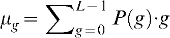
Here hg denotes the number of pixels with grey level g and M denotes the total number of pixels in the image. The mean grey level _g can be calculated using the grey level density function Pg Equation 3 where L denotes the number of grey levels present in the image.

(3)

Further, the SD of grey levels _g can be calculated from the grey level density function Pg

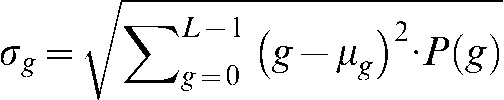(4)

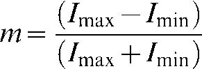
The modulation m or MTF is defined as

(5)

where I_max denotes the maximum intensity or grey level found in region of interest g_max and I_min denotes the minimum intensity or grey level g_min found in the region of interest.

A common definition of an exponential function to describe MTF is a graph of the form

(6)

Here A denotes the initial value at position x0, while y denotes the value of the function found in position x and e^b describes the growth of the function, which means a decrease for negative values of b.

References

- 1.Farman T, Vandre R, Pajak JC, Miller S, Lempicki A, Farman AG. Effects of scintillator on the modulation transfer function (MTF) of a digital imaging system. Oral Surg Oral Med Oral Pathol Oral Radiol Endod 2005;99:608–611 [DOI] [PubMed] [Google Scholar]
- 2.Workman A, Brettle D. Physical performance measures of radiographic imaging systems. Dentomaxillofac Radiol 1997;26:139–146 [DOI] [PubMed] [Google Scholar]
- 3.Farman T, Vandre R, Pajak JC, Miller S, Lempicki A, Farman A. Effects of scintillator on the detective quantum efficiency (DQE) of a digital imaging system. Oral Surg Oral Med Oral Pathol Oral Radiol Endod 2006;101:219–232 [DOI] [PubMed] [Google Scholar]
- 4.Vandre R, Pajak JC, Abdel-Nabi H, Farman TT, Farman AG. Comparison of observer performance in determining the position of endodontic files with physical measures in the evaluation of dental X-ray imaging systems. Dentomaxillofac Radiol 2000;29:216–222 [DOI] [PubMed] [Google Scholar]
- 5.Analoui M. Radiographic digital image enhancement. Part II: transform domain techniques. Dentomaxillofac Radiol 2001;30:65–77 [DOI] [PubMed] [Google Scholar]
- 6.Davies E. On the noise suppression and image enhancement characteristics of the median, truncated median and mode filters. Pattern Recognit Lett 1988;7:87–97 [Google Scholar]
- 7.Jähne B. Digital image processing (6th edn) Berlin, Heidelberg, New York: Springer, 2005 [Google Scholar]
- 8.Farman AG, Farman TT. A comparison of 18 different X-ray detectors currently used in dentistry. Oral Surg Oral Med Oral Pathol Oral Radiol Endod 2005;99:485–489 [DOI] [PubMed] [Google Scholar]
- 9.Haiter-Neto F, Casanova MS, Frydenberg M, Wenzel A. Task-specific enhancement filters in storage phosphor images from the Vistascan system for detection of proximal caries lesions of known size. Oral Surg Oral Med Oral Pathol Oral Radiol Endod 2009;107:116–121 [DOI] [PubMed] [Google Scholar]
- 10.Koob A, Sandern E, Hassfeld S, Staehle HJ, Eickholz P. Effect of digital filtering on measurements of the depth of approximal caries under different exposure conditions. Am J Dent 2004;17:388–393 [PubMed] [Google Scholar]
- 11.Tyndall D, Ludlow JB, Platin E, Nair M. A comparison of Kodak Ektaspeed Plus film and the Siemens Sidexis digital imaging systems for caries detection using receiver operating characteristic analysis. Oral Surg Oral Med Oral Pathol Oral Radiol Endod 1998;85:131–138 [DOI] [PubMed] [Google Scholar]
- 12.Parker JR. Algorithms for image processing and computer vision. New York: John Wiley & Sons Inc, 1999 [Google Scholar]
- 13.Davies E. Design of optimal Gaussian operators in small neighbourhoods. Image Vis Comput 1987;5:199–205 [Google Scholar]
- 14.Hodgson R, Bailey D, Naylor M, Ng A, McNeil S. Properties, implementations and applications of rank filters. Image Vision Comput 1985;3:4–14 [Google Scholar]
- 15.Jennings JAM, Charman WN. Analytic approximation of the off-axis modulation transfer function of the eye. Vision Res 1997;37:697–704 [DOI] [PubMed] [Google Scholar]
- 16.Patterson H. A further note on a simple method for fitting an exponential curve. Biometrika 1960;47:177–180 [Google Scholar]
- 17.Davies E. Median and mean filters produce similar shifts on curve boundaries. Electron Lett 1991;28:199–201 [Google Scholar]
- 18.Yin F-F, Giger ML, Doi K. Measurement of the presampling modulation transfer function of film digitizers using a curve fitting technique. Med Phys 1990;17:962–966 [DOI] [PubMed] [Google Scholar]
- 19.Kitagawa H, Farman A. Effect of beam energy and filtration on the signal-to-noise ratio of the Dexis intraoral X-ray detector. Dentomaxillofac Radiol 2004;33:21–24 [DOI] [PubMed] [Google Scholar]
- 20.Yoshioka T, Kobayashi C, Suda H, Sasaki T. Correction of background noise in direct digital dental radiography. Dentomaxillofac Radiol 1996;25:256–262 [DOI] [PubMed] [Google Scholar]
- 21.Yoshiura K, Stamatakis H, Welander U, McDavid W, Shi X-Q, Ban S, et al. Physical evaluation of a system for direct digital intra-oral radiography based on a charge-coupled device. Dentomaxillofac Radiology 1999;28:277–283 [DOI] [PubMed] [Google Scholar]
- 22.Analoui M. Radiographic image enhancement. Part I: spatial domain techniques. Dentomaxillofac Radiol 2001;30:1–9 [DOI] [PubMed] [Google Scholar]
- 23.Farman AG. Fundamentals of image acquisition and processing in the digital era. Orthod Craniofac Res 2003;6:S17–S22 [DOI] [PubMed] [Google Scholar]
- 24.Li H, Zhang H, Guo X, Hu G. Image restoration after pixel binning in image sensors. Tsinghua Sci Technol 2009;14:541–545 [Google Scholar]