

Abstract
Objectives
An algorithm and software to reduce metal artefact has been developed recently and is available in the Picasso Master 3D® (VATECH, Hwaseong, Republic of Korea), which under visual assessment produces better quality images than were obtainable previously. The objective of this in vitro study was to investigate whether the metal artefact reduction (MAR) algorithm of the Picasso Master 3D machine reduced the incidence of metal artefacts and increased the contrast-to-noise ratio (CNR) while maintaining the same gray value when there was no metallic body present within the scanned volume.
Methods
20 scans with a range of 50–90 kVp were acquired, of which 10 had a metallic bead inserted within a phantom. The images obtained were analysed using public domain software (ImageJ; NIH Image, Bethesda, MD). Area histograms were used to evaluate the mean gray level variation of the epoxy resin-based substitute (ERBS) block and a control area. The CNR was calculated.
Results
The MAR algorithm increased the CNR when the metallic bead was present; it enhanced the ERBS gray level independently of the presence of the metallic bead. The image quality also improved as peak tube potential was increased.
Conclusion
Improved quality of images and regaining of the control gray values of a phantom were achieved when the MAR algorithm was used in the presence of a metallic bead.
Keywords: cone beam computed tomography, artefact, noise
Introduction
Cone beam CT (CBCT) was introduced as an alternative to CT in diagnosing bone pathologies or dysfunctions in the maxillofacial complex.1,2 CBCT is considered to be an accurate imaging modality for dental diagnosis purposes.3,4 CBCT uses a cone-shaped beam X-ray source to collect attenuated photons on the detector and reconstruct a three-dimensional (3D) volume of the subject being imaged. The dose from CBCT is lower than that of CT when the scan is used for the same diagnostic purpose.5,6
It is well established that metallic structures cause artefacts to appear on radiographic images that interfere with the diagnostic quality of CT and CBCT images.7 The presence of metallic bodies within the maxillofacial complex of the patient causes beam hardening and streak artefacts,8 and ultimately leads to a limited diagnostic field of the images by obscuring anatomical structure, reducing the contrast between adjacent objects and impairing the detection of areas of interest.9-11
Strategies described for scatter management in CBCT include selection of object-to-detector gap,12 limiting the field of view,13 use of an antiscatter grid14-16 and use of algorithms to correct the X-ray scatter.17-19 Various methods for metal artefact reduction (MAR) on CBCT have been tested in previous studies. In one study, in which patients with metallic devices in their bodies were scanned, use of a pre-processing MAR algorithm resulted in better-quality images.20 In another, the milliampere second factor or the peak tube potential levels were increased, which led to higher-quality images because the increased beam energy was not absorbed totally by metallic structures.21,22 Many post-processing techniques for MAR, such as the use of the multiplanar reconstruction algorithm that leads to fewer artefacts on images and increases the diagnostic quality of scans, have also been tested.23,24 In these studies, the amount of metal artefact was assessed visually.
The Picasso Master 3D® (VATECH, Hwaseong, Republic of Korea) is a CBCT machine that has the option of applying an algorithm to reduce metal artefacts. The objective of this study was to investigate whether the Picasso Master 3D reduced metal artefacts and increased the contrast-to-noise ratio (CNR) while maintaining the same gray value of the structure being imaged when there was no metallic body next to it.
Experimental design and methods
The phantom used in this experiment was made of a plastic bucket filled with water, a plastic cover used as a platform and an epoxy resin-based substitute (ERBS)25 block measuring 20 × 8 × 8 mm. A hole was drilled into the middle of the ERBS block, which was fixed on a platform. The platform was fixed to the floor of the bucket, which was filled with water (Figure 1).
Figure 1.
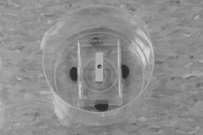
Phantom
20 scans were acquired during 1 session without moving the phantom. The scans were divided into four groups. In each group, five settings were used: 50 kVp, 60 kVp, 70 kVp, 80 kVp and 90 kVp. The level was fixed at 3 mA. For two groups, the hole made within the ERBS block was empty and filled with water; images were acquired with and without MAR. For two other groups, a metallic bead was placed within the hole of the ERBS block; images again were acquired with and without MAR. The images obtained were analysed using public domain software ImageJ (NIH Image, Bethesda, MD).
For each scan, an axial slice was saved using the same image capture tool, the same contrast and at the same axial level (Figures 2, 3). The saved images were opened with the ImageJ software, and two area histograms were computed using a macro so that all the histograms were acquired in the same location on all the images. On each analysed image, the first area histogram was acquired on the ERBS block close to the metallic bead and the second histogram was acquired over the water at a distance of 6 cm from the metal and served as a control; Figure 4 shows the areas covered by the two histograms. The mean gray level and a standard deviation (SD) were computed from the area histograms. The CNR was calculated as the difference between the mean gray levels of the ERBS portion and the control area divided by the SDs of the gray levels in the control area. A profile line covering 17 pixels was computed. The line started at the centre of the metallic bead, covered the beam hardening image and stopped on the ERBS. For each peak tube potential image, a profile line was drawn. Only two groups were considered: the scans acquired with a metallic bead without MAR and the scans acquired with a metallic bead with MAR.
Figure 2.
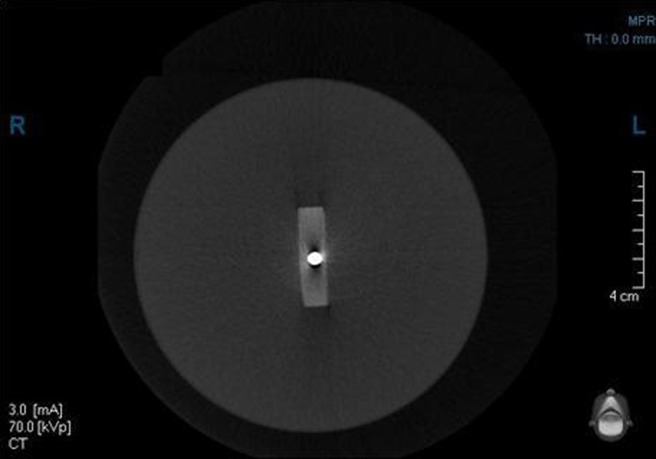
Image analysed at 70 kVp, with a metallic bead within the volume and without the use of metal artefact reduction
Figure 3.
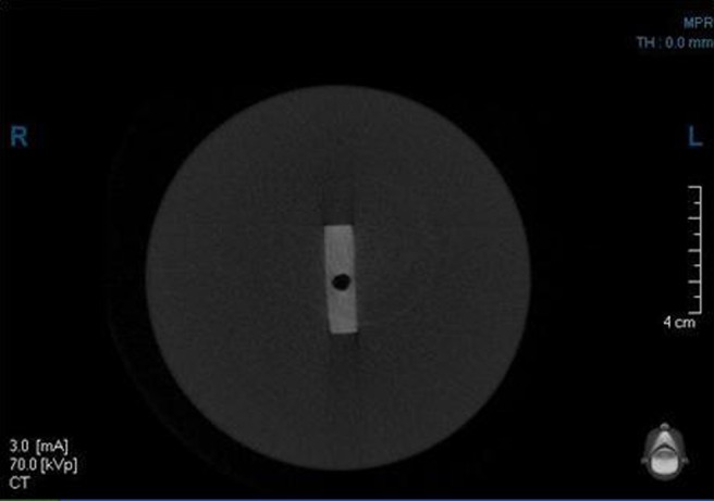
Image analysed at 70 kVp, without a metallic bead within the volume and with the use of metal artefact reduction
Figure 4.
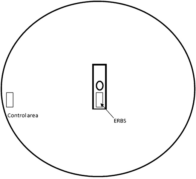
Emplacement of area histograms on the captured axial slices. The rectangles represent the areas in which the histograms were computed for each image. ERBS, epoxy resin-based substitute
Statistical methods
Variables were analysed using multiple linear regression analysis.26 A second-order model was used; that is, the model included the effects of MAR (with or without), metal (with or without), the linear and quadratic trends in tube potential (50 kVp, 60 kVp, 70 kVp, 80 kVp and 90 kVp) and the two-factor interactions MAR by metal, MAR by linear trend in peak tube potential and metal by linear trend in peak tube potential. Residual analyses indicted that the data were in reasonable conformity with the underlying assumptions of normal distribution and constant variance. The squared multiple correlation coefficient (r2) ranged from 0.95 to > 0.99, indicating a good fit of this model to the data. Profile lines were divided into 2 sets of pixel numbers: 4–6 and 8–17, based on a visual assessment. The gray level for pixels 4–6 was analysed for the effects of MAR and peak tube potential using multiple linear regression analysis. The gray level for pixels 8–17 was analysed for the effects of MAR, peak tube potential and pixel number using multiple linear regression analysis. The association with pixel number was described by the gray level at pixel number 8 and a linear trend with increasing pixel numbers. A p-value of ≤ 0.005 was considered statistically significant.
Results
Contrast-to-noise-ratio
When metal was absent, there was no difference in CNR with and without MAR (Figure 5; Table 1). Without MAR, the presence of metal was associated with a significant reduction in CNR. When metal was present, MAR significantly increased CNR, such that CNR was similar to that observed for the condition of no metal and without MAR. There was a significant linear trend in CNR with peak tube potential under all combinations of metal and use of MAR (Table 1); the CNR increased with increasing peak tube potential (Figure 5). Neither the presence of metal nor the use of MAR significantly altered the trend with peak tube potential (Table 1).
Figure 5.
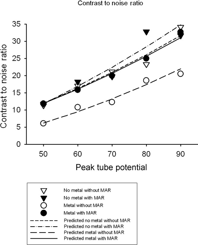
Observed and predicted contrast-to-noise ratios by metal artefact reduction (MAR; with or without), presence of metal (with or without) and peak tube potential
Table 1. Average CNR at 70 kVp and slope of the trend in CNR at 70 kVp, under the conditions “with” and “without metal” and “with” and “without MAR”.
| Ratio at 70 kVp |
Slope at 70 kVp |
||
| Metal | MAR | Mean ± SE | Slope ± SE |
| Without | Without | 21.0 ± 1.2 | 0.49 ± 0.06 |
| With | 22.4 ± 1.2 | 0.57 ± 0.06 | |
| With | Without | 13.2 ± 1.2a,b | 0.40 ± 0.06 |
| With | 20.7 ± 1.2c | 0.48 ± 0.06 |
CNR, contrast-to-noise ratio; MAR, metal artefact reduction; SE, standard error.
aSignificantly (p ≤ 0.05) different from without metal and without MAR.
bSignificantly (p ≤ 0.05) different from without metal and with MAR.
cSignificantly (p ≤ 0.05) different from with metal and without MAR.
Epoxy resin-based substitute
Mean gray value
There was a significant interaction of MAR and metal (p = 0.0001); ERBS mean was higher with than without MAR when metal was present, but lower with than without MAR when metal was absent (Figure 6; Table 2). There was a significant linear trend in ERBS mean with peak tube potential under all combinations of metal and use of MAR (Table 2); the ERBS mean decreased with increasing peak tube potential (Figure 6). Furthermore, the slope was less negative with than without MAR (interaction of MAR and linear trend with peak tube potential, p = 0.0001), and less negative when metal was present than when it was absent (interaction of metal and linear trend with peak tube potential, p = 0.0009).
Figure 6.
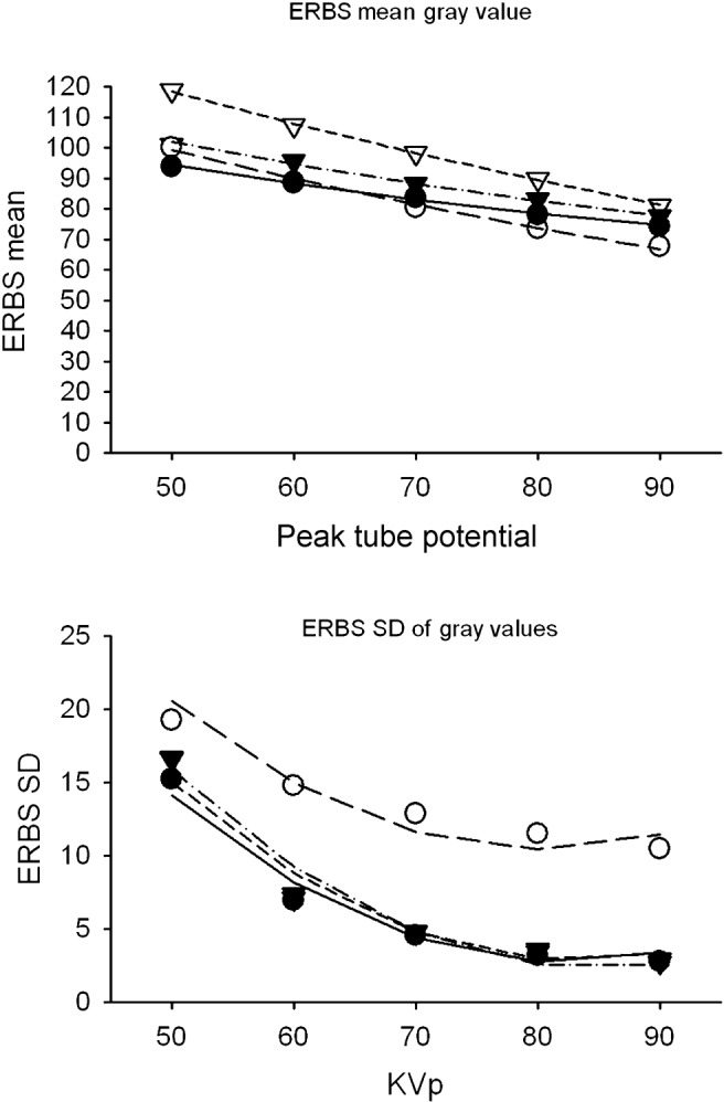
Observed and predicted epoxy resin-based substitute (ERBS) mean gray value (upper panel) and ERBS SD of gray values (lower panel), by metal artefact reduction (with or without), presence of metal (with or without) and peak tube potential. SD, standard deviation
Table 2. Average ERBS mean Gy value at 70 kVp and slope of the trend in ERBS mean at 70 kVp, under the conditions “with” and “without metal” and “with” and “without MAR”.
| Metal | MAR | ERBS mean at 70 kVp |
Slope at 70 kVp |
| Mean ± SE | Slope ± SE | ||
| Without | Without | 98.1 ± 0.4 | −0.92 ± 0.02 |
| With | 88.2 ± 0.4a | −0.60 ± 0.02a | |
| With | Without | 81.3 ± 0.4a,b | −0.81 ± 0.02a,b |
| With | 82.9 ± 0.4a–c | −0.49 ± 0.02a–c |
ERBS, epoxy resin-based substitute; MAR, metal artefact reduction; SE, standard error.
aSignificantly (p ≤ 0.05) different from without metal and without MAR.
bSignificantly (p ≤ 0.05) different from without metal and with MAR.
cSignificantly (p ≤ 0.05) different from with metal and without MAR.
SD of gray value
When metal was absent, there was no difference in ERBS SD of gray values with and without MAR (Figure 6; Table 3). Without MAR, the presence of metal was associated with a significant increase in ERBS SD. When metal was present, MAR significantly decreased ERBS SD, such that ERBS SD was similar to that observed for the condition of no metal and without MAR. There was a significant linear trend in ERBS SD with peak tube potential under all combinations of metal and use of MAR (Table 3).
Table 3. Average ERBS SD of gray values at 70 kVp and slope of the trend in ERBS SD at 70 kVp, under the conditions “with” and “without metal” and “with” and “without MAR”.
| ERBS SD at 70 kVp |
Slope at 70 kVp |
||
| Metal | MAR | Mean ± SE | Slope ± SE |
| Without | Without | 4.8 ± 0.7 | −0.29 ± 0.04 |
| With | 4.8 ± 0.7 | −0.33 ± 0.04 | |
| With | Without | 11.6 ± 0.7a,b | −0.23 ± 0.04 |
| With | 4.4 ± 0.7c | −0.27 ± 0.04 |
ERBS, epoxy resin-based substitute; MAR, metal artefact reduction; SD, standard deviation.
aSignificantly (p ≤ 0.05) different from without metal and without MAR.
bSignificantly (p ≤ 0.05) different from without metal and with MAR.
cSignificantly (p ≤ 0.05) different from with metal and without MAR.
Control
Mean gray value
The control mean was significantly lower with than without MAR (p = 0.0001), whether metal was present or absent (Figure 7; Table 4). There was a significant linear trend in control mean with peak tube potential under all combinations of metal and use of MAR (Table 4), and the slope was less negative with than without MAR (interaction of MAR and linear trend with peak tube potential; Figure 7). There was also significant curvature to the trend in control mean with peak tube potential (quadratic trend, p = 0.0001).
Figure 7.
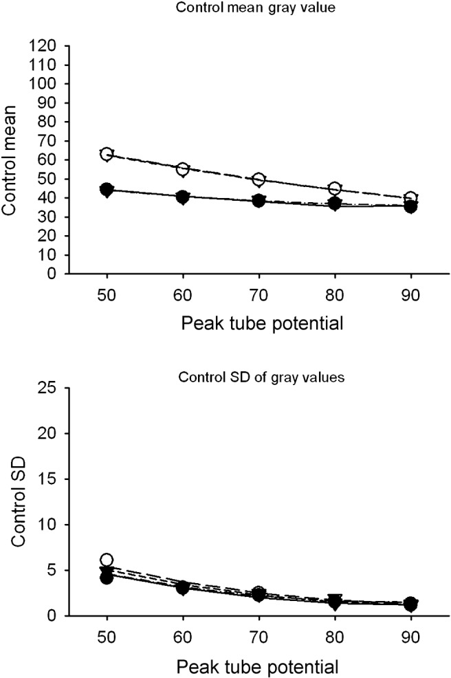
Observed and predicted control mean gray value (upper panel) and control SD of gray values (lower panel) by metal artefact reduction (with or without), presence of metal (with or without) and peak tube potential. SD, standard deviation
Table 4. Average control mean Gray value at 70 kVp and slope of the trend in control mean at 70 kVp, under the conditions “with” and “without metal” and “with” and “without MAR”.
| Control mean at 70 kVp |
Slope at 70 kVp |
||
| Metal | MAR | Mean ± SE | Slope ± SE |
| Without | Without | 49.4 ± 0.3 | −0.56 ± 0.01 |
| With | 38.3 ± 0.3a | −0.20 ± 0.01a | |
| With | Without | 49.5 ± 0.3b | −0.57 ± 0.01b |
| With | 38.2 ± 0.3a,c | −0.21 ± 0.01a,c |
MAR, metal artefact reduction; SE, standard error.
aSignificantly (p ≤ 0.05) different from without metal and without MAR.
bSignificantly (p ≤ 0.05) different from without metal and with MAR.
cSignificantly (p ≤ 0.05) different from with metal and without MAR.
SD of gray value
There were no significant effects of MAR or metal on control SD (Figure 7; Table 5). There was a significant linear trend in control SD with peak tube potential under all combinations of metal and use of MAR (Table 5), as well as a significant curvature (quadratic trend, p = 0.0001).
Table 5. Average control SD of gray values at 70 kVp and slope of the trend in control SD at 70 kVp, under the conditions “with” and “without metal” and “with” and “without MAR”.
| Control SD at 70 kVp |
Slope at 70 kVp |
||
| Metal | MAR | Mean ± SE | Slope ± SE |
| Without | Without | 2.3 ± 0.2 | −0.10 ± 0.01 |
| With | 2.2 ± 0.2 | −0.08 ± 0.01 | |
| With | Without | 2.5 ± 0.2 | −0.10 ± 0.01 |
| With | 2.0 ± 0.2 | −0.08 ± 0.01 |
MAR, metal artefact reduction; SD, standard deviation; SE, standard error.
Profile lines
The profile lines with the metallic beads without and with MAR are shown in Figure 8. The profile lines obtained for the scans acquired without MAR showed a low gray value for pixel 8, with the gray value gradually increasing with increasing pixel numbers. The profile lines obtained for the scans acquired with MAR did not show any pixel with the very low gray value. The gray values dropped from around 251 (owing to the white image of the metallic bead) to around 74 (Table 6). There was no significant change in gray value for pixel numbers 8–17 for the images with MAR (Table 6).
Figure 8.

Gray values along the profile lines for five different peak tube potential levels without and with use of the metal artefact reduction (MAR) algorithm in the presence of the metallic bead
Table 6. Gray levels along profile line without and with MAR.
| Pixel numbers 4–6 |
Pixel numbers 8–17 |
||
| Condition | Mean ± SE | Intercept (Pixel 8) ± SE | Slope ± SE |
| Metal (without MAR) | 250.9 ± 0.66 | 12.3 ± 2.4 | 6.28 ± 0.41a |
| Metal (with MAR) | 250.9 ± 0.66 | 74.2 ± 2.4b | 0.35 ± 0.41b |
MAR, metal artefact reduction; SE, standard error.
aSignificantly different from zero (p ≤ 0.005).
bSignificantly different from metal (without MAR) (p ≤ 0.005).
Discussion
The results obtained in this study show that the MAR algorithm increases the CNR significantly when used in the presence of the metallic bead. Bechara et al27 reported a similar observation using a phantom where metal was present in all scans. However, when no metal was incorporated within the ERBS, the CNR was not affected significantly with the use of the MAR algorithm. The CNR when the MAR algorithm was used in the presence of metal was similar to the control image made when the metallic bead was not present. An increase in CNR was also noted when the peak tube potential was increased. This observation is consistent with the findings of Robertson et al.22
ERBS mean gray value was higher with than without MAR when the metallic bead was present, which suggests that the noise, beam hardening and metal spray artefact result in a darker image when combined. The effects of beam hardening and noise are greater than the effect of the metal scattering that tends to increase the gray value. Similar gray value variation was found by Schulze et al,28 who used a phantom that incorporated titanium implants. They found that the gray values of the implants surrounding structures were drastically decreased.28
The ERBS mean gray value was significantly lower with than without MAR when metal was absent. The CNR was not significantly different when the metallic bead was absent. These observations indicate that the MAR algorithm did reduce the mean gray level of the ERBS material significantly but did not improve the CNR significantly; still, the CNR numbers obtained after the use of the algorithm were better compared with those obtained without it. These findings show that the noise caused an increase in the gray value of the ERBS block when metal was absent.
The ERBS was darkened with increasing peak tube potential, which is normal with increasing beam energy; the higher energy photons are absorbed less and reach the detector, causing a darker image.28 The slope of the decreasing ERBS mean gray level was less negative with than without MAR when the metallic bead was placed within the volume; the reverse was the case when the metallic body was not placed within the volume. These findings indicate that the overall noise in the images may cause the ERBS gray value to increase or decrease depending on whether or not the metallic bead is present.
The control mean gray level was significantly lower with than without MAR, whether or not the metallic bead was present. The control area was chosen to be an area occupied by water; it was not affected by the artefacts, owing to the metallic bead. These findings suggest that the noise on the image increases the gray values of the structures if those are not affected by artefacts caused by the presence of metallic structures.
The gray level variation due to noise, represented by the SD of the areas chosen, was reduced significantly only for the ERBS block when the MAR was used and the metallic bead inserted. Otherwise, the variation was not affected: for the same peak tube potential, the MAR or the presence of metal did not affect the gray level variation measured in the control area, and the same variable measured in the ERBS block area was not affected by the MAR algorithm if there was no metal used. These findings suggest that the introduction of the metallic bead within the ERBS block caused a significant increase in gray value variation, owing mainly to the addition of the beam hardening and metal scatter artefact effects. Schulze et al,28 who used a phantom that incorporated dental implants, found that the gray values of the regions adjacent to the implant images and situated in the beam hardening path varied considerably. The gray values varied most when they were computed close to the implant bodies.
The profile lines showed clearly that the beam hardening effect described by Schulze et al28 was effectively eliminated. The low gray value corresponding to a black image represents the beam hardening. The increasing gray value indicates that the beam hardening effect extended to several pixels. When the MAR was used, the transition between the metal and the ERBS gave two different groups of numbers, which were statistically the same in each group (Table 6). That fact supposes that the first one represented the gray values of the metal and the second the gray values of the ERBS without any beam hardening around the metallic bead when the MAR was used (Figure 8), and the visual comparison between Figures 2 and 9 clearly supports the results.
Figure 9.
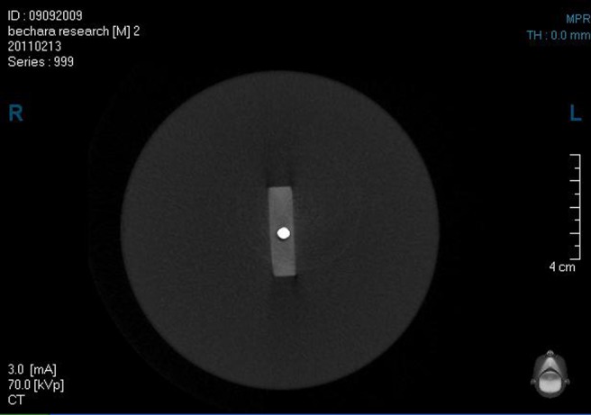
Image analysed at 70 kVp, with a metallic bead within the volume and with the use of metal artefact reduction
Clinically, the algorithm will be useful to minimize artefacts and increased noise, if any metallic structure is present within the scanned volume. However, the reconstruction time is increased whenever the MAR is used.
Conclusion
The MAR algorithm significantly reduced the noise measured on the images when a metal body was included in the phantom. Although the metal quantity was limited in the scan and a phantom was used in this in vitro study, the results appear promising. More research is needed to define the use of the algorithm clinically and to determine if it will be a reliable clinical tool to eliminate artefacts caused by high-density bodies. Despite the fact that use of the MAR algorithm involves an increased reconstruction time, it is still a useful tool in reducing metal artefacts in scans, for patients with braces undergoing orthodontic treatment or who have extensive metal-based fixed restorations in their oral cavities.
References
- 1.Arai Y, Tammisalo E, Iwai K, Hashimoto K, Shinoda K. Development of a compact computed tomographic apparatus for dental use. Dentomaxillofac Radiol 1999;28:245–248 [DOI] [PubMed] [Google Scholar]
- 2.Rigolone M, Pasqualini D, Bianchi L, Berutti E, Bianchi SD. Vestibular surgical access to the palatine root of the superior first molar: “low-dose cone-beam” CT analysis of the pathway and its anatomic variations. J Endod 2003;29:773–775 [DOI] [PubMed] [Google Scholar]
- 3.Ghaeminia H, Meijer GJ, Soehardi A, Borstlap WA, Mulder J, Bergé SJ. Position of the impacted third molar in relation to the mandibular canal. Diagnostic accuracy of cone beam computed tomography compared with panoramic radiography. Int J Oral Maxillofac Surg 2009;38:964–971 [DOI] [PubMed] [Google Scholar]
- 4.Chen Q, Liu DG, Zhang G, Ma XC. Relationship between the impacted mandibular third molar and the mandibular canal on panoramic radiograph and cone beam computed tomography. Zhonghua Kou Qiang Yi Xue Za Zhi 2009;44:217–221 [PubMed] [Google Scholar]
- 5.Bianchi S, Anglesio S, Castellano S, Rizzi L, Ragona R. Absorbed dose and risk in implant planning: comparison between spiral CT and cone beam CT. Dentomaxillofac Radiol 2001;30:S28 [Google Scholar]
- 6.Tsiklakis K, Donta C, Gavala S, Karayianni K, Kamenopoulou V, Hourdakis CJ. Dose reduction in maxillofacial imaging using low dose cone beam CT. Eur J Radiol 2005;56:413–417 [DOI] [PubMed] [Google Scholar]
- 7.Sanders MA, Hoyjberg C, Chu CB, Leggitt VL, Kim JS. Common orthodontic appliances cause artefacts that degrade the diagnostic quality of CBCT images. J Calif Dent Assoc 2007;35:850–857 [PubMed] [Google Scholar]
- 8.Draenert FG, Coppenrath E, Herzog P, Müller S, Mueller-Lisse UG. Beam hardening artefacts occur in dental implant scans with the NewTom cone beam CT but not with the dental 4-row multidetector CT. Dentomaxillofac Radiol 2007;36:198–203 [DOI] [PubMed] [Google Scholar]
- 9.Webber RL, Tzukert A, Ruttimann The effects of beam hardening on digital subtraction radiography. J Periodontal Res 1989;24:53–58 [DOI] [PubMed] [Google Scholar]
- 10.Barrett JF, Keat N. Artefacts in CT: recognition and avoidance. Radiographics 2004;24:1679–1691 [DOI] [PubMed] [Google Scholar]
- 11.Niu T, Sun M, Star-Lack J, Gao H, Fa Q, Zhu L. Shading correction for on-board cone-beam CT in radiation therapy using planning MDCT images. Med Phys 2010;37:5395–5406 [DOI] [PubMed] [Google Scholar]
- 12.Siewerdsen JH, Jaffray DA. Optimization of x-ray imaging geometry (with specific application to flat-panel cone-beam computed tomography). Med Phys 2000;27:1903–1914 [DOI] [PubMed] [Google Scholar]
- 13.Siewerdsen JH, Jaffray DA. Cone-beam computed tomography with a flat-panel imager: magnitude and effects of X-ray scatter. Med Phys 2001;28:220–231 [DOI] [PubMed] [Google Scholar]
- 14.Wiegert J, Bertram M, Schaefer D, Conrads N, Timmer J, Aach T, et al. Performance of standard fluoroscopy antiscatter grids in flat-detector-based cone-beam CT. Proc SPIE Medical Imaging 2004;5368:67–68 [Google Scholar]
- 15.Siewerdsen JH, Moseley DJ, Bakhtiar B, Richard S, Jaffray DA. The influence of antiscatter grids on soft-tissue detectability in cone-beam computed tomography with flat-panel detectors. Med Phys 2004;31:3506–3520 [DOI] [PubMed] [Google Scholar]
- 16.Endo M, Tsunoo T, Nakamori N, Yoshida K. Effect of scattered radiation on image noise in cone beam CT. Med Phys 2001;28:469–474 [DOI] [PubMed] [Google Scholar]
- 17.Seibert JA, Boone JM. X-ray scatter removal by deconvolution. Med Phys 1988;15:567–575 [DOI] [PubMed] [Google Scholar]
- 18.Spies L, Evans PM, Partridge M, Hansen VN, Bortfeld T. Direct measurement and analytical modeling of scatter in portal imaging. Med Phys 2000;27:462–471 [DOI] [PubMed] [Google Scholar]
- 19.Spies L, Ebert M, Groh BA, Hesse BM, Bortfeld T. Correction of scatter in megavoltage cone-beam CT. Phys Med Biol 2001;46:821–33 [DOI] [PubMed] [Google Scholar]
- 20.Mahnken AH, Raupach R, Wildberger JE, Jung B, Heussen N, Flohr TG, et al. New algorithm for metal artefact reduction in computed tomography: in vitro and in vivo evaluation after total hip replacement. Invest Radiol 2003;38:769–775 [DOI] [PubMed] [Google Scholar]
- 21.Vande Berg B, Malghem J, Maldague B, Lecouvet F. Multi-detector CT imaging in the postoperative orthopedic patient with metal hardware. Eur J Radiol 2006;60:470–479. [DOI] [PubMed] [Google Scholar]
- 22.Robertson DD, Weiss PJ, Fishman EK, Magid D, Walker PS. Evaluation of CT techniques for reducing artefacts in the presence of metallic orthopedic implants. J Comput Assist Tomogr 1988;12:236–241 [DOI] [PubMed] [Google Scholar]
- 23.Kalender WA, Hebel R, Ebersberger J. Reduction of CT artefacts caused by metallic implants. Radiology 1987;164:576–577 [DOI] [PubMed] [Google Scholar]
- 24.Fishman EK, Magid D, Robertson DD, Brooker AF, Weiss P, Siegelman SS. Metallic hip implants: CT with multiplanar reconstruction. Radiology 1986;160:675–81 [DOI] [PubMed] [Google Scholar]
- 25.White DR, Martin RJ, Darlison R. Epoxy resin based tissue substitutes. Br J Radiol 1977;50:814–21 [DOI] [PubMed] [Google Scholar]
- 26.Draper NR, Smith H. Applied Regression Analysis. 3rd edn John Wiley & Sons: New York, NY; 1998 [Google Scholar]
- 27.Bechara BB, Moore WS, McMahan CA, Noujeim M. Metal artefact reduction with cone beam computed tomography: an in vitro study. Dentomaxillofac Radiol 2012;41:248–253 [DOI] [PMC free article] [PubMed] [Google Scholar]
- 28.Schulze RK, Berndt D, d'Hoedt B. On cone-beam computed tomography artefacts induced by titanium implants. Clin Oral Implants Res 2010;21:100–7 [DOI] [PubMed] [Google Scholar]