Modulation transfer function evaluation of cone beam computed tomography for dental use with the oversampling method

Abstract

Objectives

The aim was to investigate the possibility of evaluating the modulation transfer function (MTF) of cone beam CT (CBCT) for dental use using the oversampling method.

Methods

The CBCT apparatus (3D Accuitomo) with an image intensifier was used with a 100 μm tungsten wire placed inside the scanner at a slight angle to the plane perpendicular to the plane of interest and scanned. 200 contiguous reconstructed images were used to obtain the oversampling line-spread function (LSF). The MTF curve was obtained by computing the Fourier transformation from the oversampled LSF. Line pair tests were also performed using Catphan®.

Results

The oversampling method provided smooth and reproducible MTF curves. The MTF curves revealed that the spatial resolution in the z-axis direction was significantly higher than that in the axial direction. This result was also confirmed by the line pair test.

Conclusions

MTF analysis was performed successfully using the oversampling method. In addition, this study clarified that the 3D Accuitomo had high spatial resolution, especially in the z-axis direction.

Introduction

The cone beam CT (CBCT) technique has been widely introduced into dental practice and is accepted as a useful method in diagnosing dentomaxillofacial lesions1, 2 and planning dental implants.3 One of the advantages of CBCT is its high spatial resolution; however, there have been few reports that have evaluated the spatial resolution of the CBCT systems.4, 5

The modulation transfer function (MTF), which is calculated from the line-spread function (LSF), is the established method of characterizing the spatial response of an imaging system. To obtain the LSF, there are several techniques, including using a fine wire, narrow slits or an edge phantom. However, because CBCT systems are designed to use lower radiation doses than medical CT instruments,6 they provide relatively noisy images.7 Thus, it has been difficult to obtain stable and robust LSF values. In addition, there is a problem due to aliasing from the finite sampling in digital imaging systems.8 Recently, to overcome these issues, oversampling has typically been used.9

The aim of this study was to investigate the possibility of evaluating the MTF of CBCT using an oversampling method. This study was formulated under the hypothesis that this method could provide precise and reliable data of spatial resolution in both the x- (or y-) and the z-axis directions.

Materials and methods

CBCT and data acquisition

A 3D Accuitomo CBCT apparatus with an image intensifier (Morita Corp., Kyoto, Japan) and a minute voxel size of 0.125 mm3 was used. The imaging area was a cylinder with a diameter of 40 mm (320 voxels) and a height of 30 mm (240 voxels).

A 100 μm tungsten wire phantom (Morita Corp., X001-99520-400) was placed inside the scanner at a central position and scanned. For measurement of the axial and z-axis MTFs, the phantom was located with the wire parallel and perpendicular, respectively, to the rotation axis of the CBCT. In this phantom, the wire had a slight angle and was off-centre from the phantom axis, and the measurements of the MTF were obtained at an off-centre position (the radial distance was approximately 7.2 mm). The scans were performed at a tube voltage of 60 kV and a tube current of 1–2 mA for an exposure time of 17 s. Five scans were performed for each acquisition configuration. After scanning, 200 contiguous sectional images in the axial and z-axis directions with a slice width of 0.5 mm and an increment of 0.125 mm were reconstructed with a default reconstruction filter. The image data were exported as digital imaging and communications in medicine (DICOM) image files using dedicated iView software (Morita Corp.), and used for the MTF evaluation.

To visually determine the spatial resolution, the high-resolution insert of the Catphan® 500 (Phantom Laboratories, Salem, NY) was also scanned. The scans were performed at 80 kV, 10 mA and for 17 s. Sectional images were reconstructed in the axial and z-axis directions with a slice width of 0.5 mm, the bar patterns and the corresponding spatial frequencies were assessed in lp cm⁻¹ that could be resolved.

Oversampling method

Once the image data were obtained, the MTF was first computed by integrating a region of interest (ROI), (30×30 pixels) surrounding the wire to produce the LSF, as shown in Figure 1. Next, the base of the LSF was normalized to zero and, finally, the MTF was determined by computing the fast Fourier transformation of the normalized LSF. Because the MTF from one CT slice is neither stable or robust, owing to image noise and/or the finite sampling of the wire,10 an oversampling method was used in this study.9 Namely, the tungsten wire was placed at a slight angle to the plane perpendicular to the plane of interest and was scanned. The 200 contiguous images were then reconstructed with a default reconstruction filter, and LSFs were computed for each slice. The centre of mass for each LSF was computed as described previously9 and plotted as a function of the slice number (S), as shown in Figure 2a. Linear regression was calculated to fit these points, and the resulting regression parameters were used to determine the LSF centres along the CT slices, which were then used for the oversampling of LSFs. The oversampled LSFs were rebinned to one-tenth (or one-fifth in the case of the z-axis direction) of a pixel width and averaged, as shown in Figure 2b. From the resultant LSF, the MTF was calculated. To set the ROI on the images and crop the ROI images, a DICOM viewer, OsiriX, and plug-in software, CMIV_CTA_TOOLS, were used (http://www.osirix-viewer.com/index.html). For conversion from cropped images to text image files, ImageJ software was used (http://rsb.info.nih.gov/ij/). The oversampling processes of LSFs were performed with a special program made by R,11 and the oversampled LSF normalization and the Fourier transformation were calculated using Microsoft Excel (Microsoft Corp., Redmond, WA).

Figure 1.

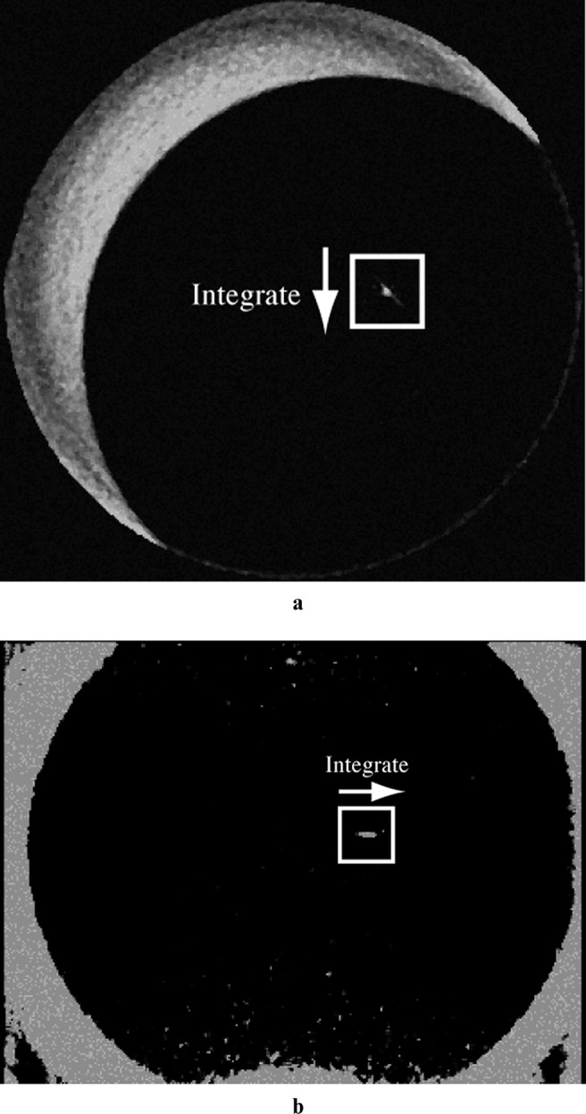
Reconstructed images of the 100 μm tungsten wire. (a and b) Images in the axial and z-axis directions, respectively. The white squares surrounding the wire represent the region of interest, the size of which is 30×30 pixels. For the modulation transfer function determination, the line-spread function was obtained by integrating in the direction illustrated by the arrows

Figure 2.

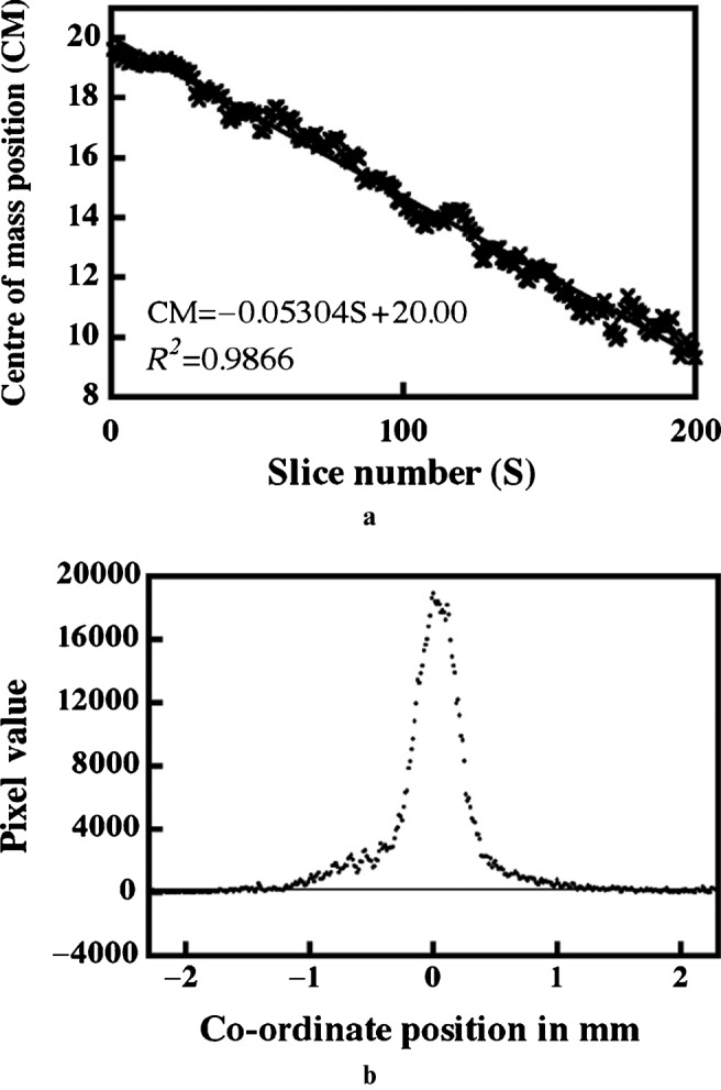
The oversampling method and its result. (a) A relationship between slice number (S) and the centre of mass position of 200 contiguous images, which enabled the determination of the linear regression parameters. Based on these parameters, the 200 line-spread functions (LSFs) were rebinned to one-tenth of a pixel width (0.0125 mm), and the averaged LSFs obtained are shown in (b)

Statistical analysis

The unpaired Student's t-test was used and P-values less than 0.01 were considered significantly different.

Results

The MTF curves in the axial and z-axis directions are shown in Figure 3. The data are represented as the mean and standard deviation (SD). Although there were some variations for the points in the axial direction, the MTF in the z-axis direction was higher than that in the axial direction. The values of ρ₅₀ and ρ₁₀ were determined, at which the MTF dropped to 50% and 10%, respectively, of its value at 0 lp cm⁻¹, as listed in Table 1. With either ρ₅₀ or ρ₁₀, the spatial frequencies in the z-axis direction were significantly greater (P-values were 0.00000061 and 0.0000046, respectively) than those in the axial direction.

Figure 3.

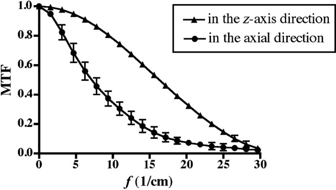
Modulation transfer function curves of cone beam CT in the axial and z-axis directions are illustrated. The data are represented as the mean and SD of five independent measurements

Table 1. Spatial frequencies in the axial and the z-axis modulation transfer functions (MTFs).

	Spatial frequency
	ρ50 in 1 cm−1	ρ10 in 1 cm−1
In the axial direction	7.1 ± 0.8 (6.4–8.3)	17.5 ± 1.3 (15.8–16.7)
In the z-axis direction	16.3 ± 0.4∗ (16.5–19.7)	26.4 ± 0.8∗ (25.6–27.8)

∗P < 0.01

ρ₅₀ and ρ₁₀ are the spatial frequencies at which the MTF has dropped to 50% and 10% of its value at 0 lp cm⁻¹

The values in parentheses represent the range

The images of the line pair test using Catphan® are shown in Figure 4. As predicted by the analysis of the MTF curves, 19–21 lp cm⁻¹ (Figure 4b: A, B and C) could be differentiated in the z-axis direction image, which reflected the high MTF in the z-axis direction; 21 lp cm⁻¹ (Figure 4a: C) could not be resolved in the axial image.

Figure 4.

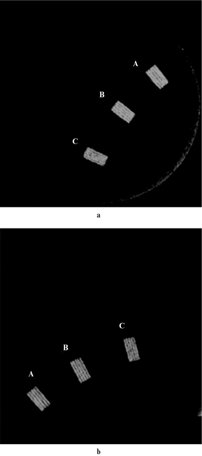
Axial (a) and z-axis (b) images of the high-resolution insert of Catphan®. The window width and window level were set to 3600 and 2400, respectively, in both images. (A), (B) and (C) represent 19, 20 and 21 lp cm⁻¹, respectively. In (b), 19–21 lp cm⁻¹ can be resolved, whereas, in (a), 21 lp cm⁻¹ cannot be resolved. These results are consistent with those by the analysis of the MTF curves shown in Figure 3

Discussion

To evaluate the spatial resolution of a CBCT system for dental use, this study applied the oversampling method and determined MTF curves. The obtained MTF curves were smooth and suggested high reproducibility for five independent measurements. There were some variations in the MTF in the axial direction, which was considered to be due to metal artefacts around the wire. In Figure 1a, artefacts could be found as 2 spindles radiating from the wire and arose irregularly through the 200 images. Generally, to reduce the number of artefacts, it is effective to increase the radiation dose for scanning and/or compile contiguous images.7 In this study, the wire in the axial direction was scanned with 60 kV and 2 mA, which was the maximum radiation dose (34 mAs), to obtain the wire images, and the oversampling method was used. Therefore, it was considered a limitation to obtain the best MTF curve with this method. The maximum variation was approximately 11% at the parameter of ρ₅₀ in the axial direction. On the other hand, Figure 1b shows that there were metal artefacts spreading in the horizontal (axial) direction but never in the vertical (z-axis) direction. This finding explains the better reproducibility in the z-axis direction than that in the axial direction. As shown in Figure 3, the SD bars in the z-axis direction were very small. The variations in ρ₅₀ and ρ₁₀ were within 0.02–0.03%. This study presents the MTF results obtained at only specific positions. It is generally said that CT is often subject to space-variance, as Kwan et al9 indicated. However, the present study could not find any significant differences at the different locations in the field of view of the 3D Accuitomo. It was considered that this is because the 3D Accuitomo has a limited field of view, with a diameter of 4 cm and a height of 3 cm.

In this study, a phantom using a 100 μm tungsten wire was used, and the authors did not deconvolve the wire from the MTF. Thus, the potential error rate should be considered, and this was estimated by calculation of a 100-μm-wide rectangle that would be the projection image of a 100 μm wire. When the MTF was normalized to 1 at a frequency (f) of 0, the calculated MTFs were 0.9986, 0.99, 0.978 and 0.962 at 7.8. 15.6, 23.4 and 31.2 cm⁻¹, respectively. Namely, there is a maximum of only 4% underestimation for MTF measurements using this method. It was considered that the errors were negligible.

The results of the MTF analysis suggested that the spatial resolution in the z-axis direction was higher than that in the axial direction. This fact was confirmed by the line pair test using Catphan®. The value of ρ₁₀ in 1 cm⁻¹ was 17.5 ± 1.3 in the axial direction, which was nearly consistent with the results of the line pair test showing a resolution up to 19–20 lp cm⁻¹. In the z-axis direction, the value of ρ₁₀ in 1 cm⁻¹ was 26.4 ± 0.8, suggesting that at least 25 lp cm⁻¹ should be resolved theoretically. However, Catphan® does not contain a high-resolution insert, so this method was not able to verify this hypothesis.

There have been few reports evaluating the MTF of CBCT systems. Arai et al4 developed CBCT for dental use, Ortho-CT, and reported that the spatial resolution limit of the apparatus was about 20 lp cm⁻¹ in both the vertical and horizontal directions on the basis of MTF analysis. However, their MTF curves did not seem to be as smooth because they were probably determined from only one CT slice image, which might result in equal spatial resolution in two directions, and this result should be validated further. Araki et al5 evaluated the MTFs of another CBCT apparatus, CB MercuRay, and reported similar results. They used the presampled MTF method with a thin metal foil and yielded smooth MTF curves. This method is technically difficult in the respect that the geometrical settings of the foil phantom must be placed perfectly vertical to the measurement planes. When the phantom declines slightly, the resultant MTF curve is lower than that in the precise settings. Kwan et al9 evaluated the MTF with a cone beam breast CT scanner using the oversampling method. They concluded that the MTF in the z-axis direction was better than the axial plane MTF, and proposed that the axial image was affected by the reconstructed filter, but hardly in the z-direction as an explanation. In principle, because CBCT is a cluster scanning system and the data are obtained by a single rotation of a two-dimensional sensor, so the spatial resolution in the z-axis could be potentially close to the physical resolution in the longitudinal direction. In contrast, the axial images need a reconstruction filter algorithm, so the spatial resolution should be reduced because of the algorithm, and not only because of the physical resolution.

In this study, the MTF of a CBCT system was analysed successfully using the oversampling method. This is the first definitive evaluation of CBCT for dental use because the obtained MTF curves were smooth and reproducible, which enabled the comparison of spatial resolutions in different directions. It was clarified that the 3D Accuitomo instrument had high spatial resolution, especially in the z-axis direction. Although further studies with other CBCT instruments may be required, it may be one of the peculiar characteristics of CBCT for dental use that the MTF in the z-axis direction is higher than that in the axial direction.

References

- 1.Tantanapornkul W, Okouchi K, Fujiwara Y, Yamashiro M, Maruoka Y, Ohbayashi N., et al A comparative study of cone-beam computed tomography and conventional panoramic radiography in assessing the topographic relationship between the mandibular canal and impacted third molars. Dentomaxillofac Radiol 2007;103:253–259 [DOI] [PubMed] [Google Scholar]
- 2.Momin MA, Okouchi K, Watanabe H, Imaizumi A, Omura K, Amagasa T, et al. Diagnostic accuracy of cone-beam CT in the assessment of mandibular invasion of lower gingival carcinoma: comparison with conventional panoramic radiography. Eur J Radiol 2009;72:75–81 [DOI] [PubMed] [Google Scholar]
- 3.Loubele M, Guerrero ME, Jacobs R, Suetens P, van Steenberghe D. A comparison of jaw dimensional and quality assessments of bone characteristics with cone-beam CT, spiral tomography, and multi-slice spiral CT. Int J Oral Maxillofac Implants 2007;22:446–454 [PubMed] [Google Scholar]
- 4.Arai Y, Tammisalo E, Hashimoto K, Shinoda K. Development of a compact computed tomographic apparatus for dental use. Dentomaxillofac Radiol 1999;28:245–248 [DOI] [PubMed] [Google Scholar]
- 5.Araki K, Maki K, Seki K, Sakamaki K, Harata Y, Sakaino R, et al. Characteristics of a newly developed dentomaxillofacial X-ray cone beam CT scanner (CB MercuRay): system configuration and physical properties. Dentomaxillofac Radiol 2004;33:51–59 [DOI] [PubMed] [Google Scholar]
- 6.Ludlow JB, Ivanovic M. Comparative dosimetry of dental CBCT and 64-slice CT for oral and maxillofacial radiology. Oral Surg Oral Med Oral Pathol Oral Radiol Endod 2008;106:106–114 [DOI] [PubMed] [Google Scholar]
- 7.Hanson KM. Noise and contrast discrimination in computed tomography. In: Newton TH, Potts G (eds). Radiology of the skull and brain. Technical aspects of computed tomography. St. Louis: CV Mosby, 1981, pp 3941–3955 [Google Scholar]
- 8.Fujita H, Tsia D, Itoh K, Doi J, Morishita K, Ueda K, et al. A simple method for determining the modulation transfer function in digital radiography. IEEE Trans Med Imaging 1992;11:34–39 [DOI] [PubMed] [Google Scholar]
- 9.Kwan AL, Boone JM, Yang K, Huang SY. Evaluation of the spatial resolution characteristics of a cone-beam breast CT scanner. Med Phys 2007;34:275–281 [DOI] [PubMed] [Google Scholar]
- 10.Nickoloff EL, Riley R. A simplified approach for modulation transfer function determinations in computed tomography. Med Phys 1985;12:437–442 [DOI] [PubMed] [Google Scholar]
- 11.R DevelopmentCoreTeam R: A language and environment for statistical computing. Vienna: R Foundation for Statistical Computing, 2008. http://www.R-project.org. [Google Scholar]