Non-parametric estimation of a time-dependent predictive accuracy curve

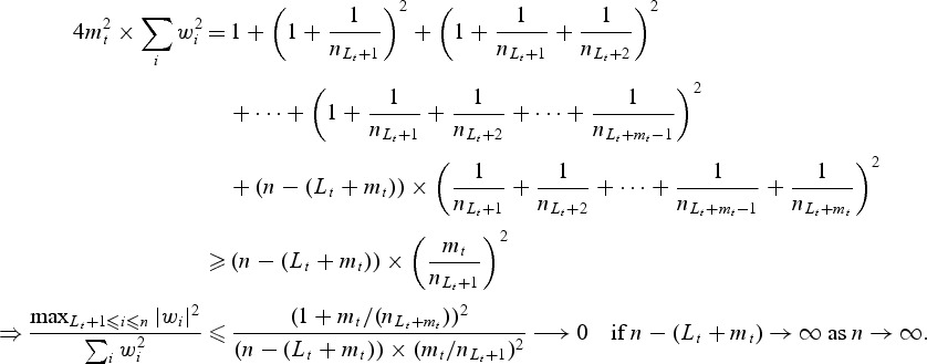
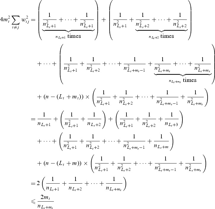
Abstract

A major biomedical goal associated with evaluating a candidate biomarker or developing a predictive model score for event-time outcomes is to accurately distinguish between incident cases from the controls surviving beyond t throughout the entire study period. Extensions of standard binary classification measures like time-dependent sensitivity, specificity, and receiver operating characteristic (ROC) curves have been developed in this context (Heagerty, P. J., and others, 2000. Time-dependent ROC curves for censored survival data and a diagnostic marker. Biometrics 56, 337–344). We propose a direct, non-parametric method to estimate the time-dependent Area under the curve (AUC) which we refer to as the weighted mean rank (WMR) estimator. The proposed estimator performs well relative to the semi-parametric AUC curve estimator of Heagerty and Zheng (2005. Survival model predictive accuracy and ROC curves. Biometrics 61, 92–105). We establish the asymptotic properties of the proposed estimator and show that the accuracy of markers can be compared very simply using the difference in the WMR statistics. Estimators of pointwise standard errors are provided.

1. Introduction

In order to choose among candidate management options and to make medical decisions, the prediction of an individual’s future health status is often necessary. The predictive objective can frequently be evaluated by quantifying how well a set of potential biomarkers or a model score can predict those subjects who subsequently experience a primary transition of health status such as the onset of disease or progression to death. One area of clinical management where predictive models or markers are used to guide treatment decisions is the general area of organ transplantation. For example, in staging patients for lung transplantation, the lung allocation score is used to prioritize transplantation candidates (Gries and others, 2010). In this setting, a good predictive model or marker would accurately identify those subjects who are still under study but otherwise likely to die in the near future (imminent “cases”), yet not falsely identify subjects who will not have an urgent need for transplantation (near term “controls”). A second example comes from liver disease where the model for end-stage liver disease (MELD) score is used for treatment decision making. As reviewed by (Coombes and Trotter (2005 p. 87) “The MELD score has emerged as an excellent predictor of short-term mortality in patients with advanced liver disease, and patients listed for liver transplantation are now ranked on their respective MELD scores.” One useful descriptive summary of the potential performance of the MELD score would be to use cohort data and show where incident death cases actually rank among their corresponding risk-set members. If the MELD score were an ideal marker, then incident cases at any time would always rank higher than all of their corresponding risk-set members. The goal of this manuscript is to show that such an empirical risk-set ranking of incident cases is directly linked to previously proposed time-dependent accuracy concepts, and also to show that risk-set ranking provides the basis for non-parametric estimation of time-dependent accuracy summary measures.

To incorporate time into predictive classification criterion, time-dependent versions of sensitivity and specificity have been proposed (Heagerty and others, 2000; Heagerty and Zheng, 2005). Time-dependent receiver operating characteristic (ROC) curves and area under the ROC curve (AUC) functions can characterize how well candidate markers can distinguish between those cases who experience a clinical transition from those subjects who remain event-free. Time-dependent measures describe the accuracy of a model score sequentially over time as opposed to simply providing an overall summary measure of the predictive accuracy like the C-index (Harrell and others, 1982) or some of its recent extensions (Antolini and others, 2005; Gonen and Heller, 2005). Heagerty and Zheng (2005) proposed a semi-parametric estimator for the time-dependent summary curve AUC(t). However, their estimation was “indirect” in that first estimates of time-dependent ROC curves for all observed event times are obtained. Each time-dependent ROC curve can then be integrated to provide an estimate of AUC(t).

The goal of this manuscript is to propose an alternative direct non-parametric estimator of the time-dependent accuracy curve, AUC(t). Relative to the semi-parametric estimators proposed by Heagerty and Zheng (2005), a non-parametric estimator has the major advantage of not requiring specification of a conditional hazard regression model linking the marker to the event time, and therefore the proposed methods provide valid inference for AUC(t) under minimal assumptions. In addition, we provide analytic approximations for point-wise standard errors and thus permit inference without needing to employ resampling methods.

To motivate the proposed non-parametric approach, we first note that an estimator of AUC that is commonly used in case–control studies is the empirical proportion of concordant case–control pairs (C-index). Specifically, concordance counts the pairs whose marker orderings correctly reflect the ordering of their outcomes. Such a non-parametric approach can be considered for each riskset in a time-to-event setting with incident cases. However, frequently only a small number of subjects experience an event at any given time, t, and therefore some smoothing is warranted to provide function estimation with desirable statistical properties. In this article, we propose the local rank-based concordance estimation using weighted U-statistics. We introduce the notation and motivate the estimation of the time-dependent AUC curve as a locally weighted concordance measure. We detail the large-sample properties of the proposed non-parametric estimator and discuss the estimation of asymptotic standard errors in Section 2. We also propose methods for comparison of correlated markers using difference in AUC curves. Finally, we examine the finite sample properties of the proposed AUC function estimator as well as the difference estimator via simulation studies in Section 4. In Section 5, we apply the method to Mayo PBC data and Breast cancer mortality data. We conclude the article with a brief discussion (Section 6).

2. Estimation of a time-dependent accuracy function

2.1. Notation

Let n denote the total number of subjects in the study. Let T_i and C_i denote the survival time and censoring time for subject i. We assume that T₁,T₂,…,T_n are independent and identically distributed and so are C₁,C₂,…,C_n. For each subject, T_i is assumed to be independent with C_i. Let denote the indicator function. We observe the follow-up time Z_i = min{T_i,C_i} and the censoring indicator . Let denote the at-risk indicator. Let M₁,M₂,…,M_n denote independently distributed baseline markers for the subjects. Note that the marker may be a single covariate X or based on a set of (time-independent or time-dependent) covariates X₁,X₂,…,X_p, via a possibly time-dependent score generated through any regression or predictive model such as the proportional hazard model. Higher marker values are assumed to be more indicative of disease and therefore shorter survival time. Let denotes the subjects that are in the riskset at time t. Among the subjects in , we denote by the subjects who had an event at t or cases: . The subjects who did not have an event by t are the controls: . We denote by n_t the size of the control set at time t: and . 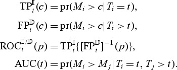Thus, cases are incident () cases and controls are dynamic () controls Heagerty and Zheng (2005). In the next subsection, we introduce non-parametric, time-dependent, concordance measures for a baseline marker and motivate the modification for a longitudinal marker. The following definitions of time-dependent accuracy are adopted:

2.2. Weighted mean rank: a local concordance measure

We first consider a baseline marker M and introduce a new approach to evaluate the predictive accuracy of this marker for a time-to-event outcome T by extending the standard binary diagnostic accuracy summaries. Note that the risk-set at time t can be represented as . A non-parametric estimator of AUC that is frequently used in case–control studies is the proportion of concordant case–control pairs, i.e. proportion of case–control pairs where the marker value for the case is higher than the marker value for the control. This statistic can be adapted in this situation using the incident case and dynamic control definition:

Note that at a given event time t, A(t) can be considered as an estimator of a time-dependent concordance measure AUC(t) = pr(M_i>M_j|T_i = t,T_j>t), which represents the area under the incident/dynamic time-dependent ROC curve defined by Heagerty and Zheng (2005). However, frequently, there are only a few cases at t and often d_t = 1. In this situation, the information within a neighborhood around t can be utilized to estimate marker concordance at t. When d_t = 1, is the rank of the case marker value among the control markers. We propose using the locally weighted mean rank (WMR) for the case markers among the available controls as an estimator of the local concordance:

where denotes a neighborhood around t. This is a nearest-neighbor estimator of the AUC and can be generalized to

where K_hn is a standardized kernel function such that .

2.3. Asymptotic distribution of WMR estimator

For simplicity, we assume that no two subjects fail at the same time and no subjects are censored. We denote the ordered observed failure times as t₍₁₎<t₍₂₎<⋯t_(M). In this section we focus on the estimation of AUC(t) at a fixed t using WMR(t). Given a bandwidth h_n, such that and , we restrict our attention to a neighborhood around t: and . Furthermore, we assume that, for any fixed t, the observed number of subjects at risk, n_t+1, is O(n) (proportional to the sample size) and therefore . This assumption results when a fixed censoring distribution is assumed, and when t is within the support of the event time and censoring time distributions.

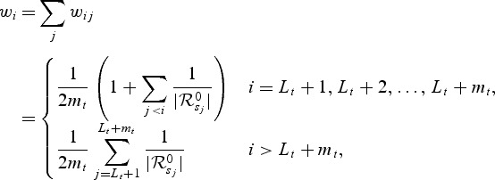
In order to detail the large sample properties of the proposed local estimator, we define the indices of ordered event times that fall within the neighborhood . Let L_t = |{t_(j):t_(j)<t − h_n}| denote the number of failures that are observed before the start of the neighborhood of interest (e.g. before time t − h_n). The indices of the observed failure times within the neighborhood are then L_t+1,L_t+2,…,L_t+m_t and that t_(Lt+1)<t_(Lt+2)<⋯<t_(Lt+mt) are the corresponding unique event times within .

For the estimation of AUC(t) based on information specific to the neighborhood , any failure time that is observed after the right boundary of the neighborhood (e.g. >t_(Lt+mt)) is only used as a “control” for all of the observed events in the neighborhood. Therefore, we effectively censor subjects surviving past t_(Lt+mt) at this time.

First, we also assume that all event times are reordered such that for the ith subject with event time T_i and marker M_i this individual corresponds to the ordered time T_i = t_(i). Secondly, for local estimation at time t, all subjects with event times beyond the right edge of the window contribute only as local “control” observations and we use only the information that they have T_i>t_(Lt+mt). We can therefore equivalently represent the WMR estimator in terms of the locally censored observations :

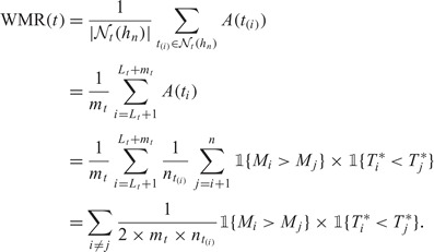Note that for two subjects i and j with i,j>L_t+m_t, we cannot order the failure times, Hence, we assume that and .

From the above representation of the WMR(t), it can be seen that WMR(t) is a linear transformation of weighted U-statistic: WMR defined as

where sgn(x) = 1 if x>0 and sgn(x) = − 1 if x<0, R_i is the rank of the marker M corresponding to the ith-ordered observed failure time and . Since higher marker values are more indicative of a shorter survival time, the definition of U is slightly different than the standard U-statistic.

Conditioning on the event times, we can show that standardized WMR(t) has an asymptotic normal distribution since, in this case, the weights w_ij can be treated as constants. We state the result in the following theorem, and explicitly denote the sample size for the proposed estimator using the notation WMR_n(t):

Theorem 1 —

Suppose when where n − (L_t+m_t) denotes the number of subjects surviving past t_(Lt+mt) or equivalently, surviving past t+h_n and let , . Then

where V_n = var[WMR_n(t)] given below, and b_n(t) denotes the bias: E[WMR_n(t)] = AUC(t)+b_n(t).

Proof —

See Appendix for details.

Since the WMR using a nearest-neighbor kernel is equivalent to the Nadaraya–Watson estimator, at an interior point t WMR_n(t) has a bias of for a given bandwidth h_n (Hardle 1992). Here , where AUC⁽¹⁾(t) (AUC⁽²⁾(t)) denotes the first (second) derivative of the AUC, f(⋅) denotes the probability density function of the survival time and f⁽¹⁾(⋅) denotes the first derivative. Characterization of the finite-sample bias can be used to correct confidence interval estimates to ensure proper coverage rates. Each of the elements of bias can be estimated using standard smoothing techniques. It can be shown that for a bandwidth h_n satisfying h_n = o(n^−2/5), the bias will be asymptotically negligible relative to , but using a bandwidth O(n^−1/5) is optimal for minimizing integrated mean squared error (IMSE), yet then requires the bias correction for proper confidence interval construction.

2.4. Estimation of variance

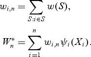
Because WMR(t) is an average of random variables, we can write

We propose the following as estimators of the variance of A(t) and covariance between A(t) and A(s), t<s:

Q_⋅(⋅) is defined in Appendix. So, . Further, , etc. are obtained using a normal approximation for the case and control markers after a rank-based Z-score transformation and then empirically estimating the parameters of the approximating normal distributions. Ultimately, our implementation of variance estimation is based solely on the marginal ranks of the marker measurements and survival times since, as we describe in the appendix, we first rank the raw marker values and then apply a Z-score transformation to these ranks. Secondly, we use a normal approximation to the conditional distributions, M*|T = t and M*|T>t, where M* denote the transformed marker values. Although the normal approximation is not an exact characterization, we have found that the approximation, coupled with the rank-based Z-score transformation, provides accurate standard error estimates for even highly skewed marginal marker distributions. Details of our simulation evaluations are presented in the next section.

2.5. Selection of bandwidth

We note that estimation of AUC via WMR is similar in spirit with several smoothing techniques that are widely used in practice and selection of a bandwidth, h_n for is important to the estimation of WMR. The optimal bandwidth balances bias and variance, and optimizes the estimation of time-dependent concordance. Since we want to estimate the time-dependent concordance, we focus on a criterion directly related to it. We adopt a bandwidth that minimizes the asymptotic IMSE of WMR:

In practice, cross-validation or a data-driven method can be employed to estimate the asymptotically optimal bandwidth.

Replacing the integration over time by a sum over k unique event times, the optimal bandwidth is a minimizer of

where

Similar to other smoothing techniques, alternative types of neighborhood selection can also be employed. For example, instead of a fixed bandwidth for the entire support, we can employ a nearest-neighbor method with fixed number of “neighbor” or failure times. Fixing the number of “neighbors” instead of a fixed bandwidth will especially be useful when either the events are sparse or the sizes of risksets are small. A cross-validation method based on IMSE can be employed to estimate the optimal number of “neighbors” as before.

3. Comparison of markers

Suppose that it is of interest to compare the two markers A (M^A) and B (M^B) for their predictive accuracy. Comparison of the AUCs for these two markers is one simple approach to determine whether marker A is more accurate than marker B in correctly classifying the incident cases and dynamic controls at t. This can be done via the difference in the WMR statistic for the respective markers. For the marker-specific AUCs at t, define dAUC(t) = AUC^A (t) − AUC^B (t) and dWMR(t) = WMR^A (t) − WMR^B (t). Then dWMR(t) can be used as an estimator of dAUC(t).

The estimation of the variance of dWMR(t) is straightforward for two uncorrelated markers since, in this case,

This is true when markers are measured on different sub-groups. However, frequently, both the markers are assessed on the same set of subjects and hence the covariance between the two WMR statistics cannot be ignored in general. For correlated markers, the variance of dWMR(t) can be written as

For estimating the covariance, one needs to evaluate terms of the form

where , etc. The estimation of these covariance terms parallels the approach for variance estimation for single marker.

An optimal bandwidth may be selected for marker comparison as before. In particular, an optimal bandwidth for marker comparison is a minimizer of

where

4. Simulation study

4.1. Single marker

To demonstrate the use of the WMR to estimate time-dependent concordance and the rank-based variance estimator, we conducted a set of simulation studies. Suppose that T denotes the (log) time until failure and M denotes the marker. We assumed that (T, M) jointly follows a bivariate normal distribution with means 0, variances 1, and correlation ρ = − 0.7. For each of N = 1000 simulated datasets, a sample of n = 200 marker values M and survival times T were generated. An additional independent censoring (log) time was generated such that either 20% or 40% subjects are censored. To estimate that WMR, a bandwidth of n ^−1/5 (b = 1) was considered. For each simulated dataset, we estimated that WMR at t = − 2.0, − 1.5,…,1.0. The average WMR over 1000 simulations, the Monte-Carlo standard deviation (MCSD), the estimated SD (EstSD) using the proposed variance estimator and the coverage can be found in Table 1. For comparison purposes, we also cite the maximum likelihood estimate (MLE) and semi-parametric estimates of time-dependent AUC as in Heagerty and Zheng (2005). Additionally, simulation results for comparison of two markers can be found in Table 2.

Table 1.

Simulation results for WMR and comparison with semi-parametric method. We assumed (log(T),M)∼N₂(0,0,1,1, − 0.7). An independent censoring time was generated such that either 20% or 40% subjects were censored. The results are based on 1000 such simulations. The MLE and semi-parametric estimates are cited from Heagerty and Zheng (2005). MCSD denotes the Monte-Carlo SD. The nominal coverage is 95.0. Estimate of integrated AUC (iAUC) and its variance is based on 10 equi-spaced quantiles of time. The variance of integrated AUC is estimated assuming a constant weight

		MLE		Semi-parametric		WMR (n = 200)
Log time	AUC(t)	Mean	SD	Mean	SD	Mean	MCSD	EstSD	Coverage
20% censoring
− 2.0	0.884	0.884	0.018	0.881	0.044	0.876	0.055	0.050	90.2
− 1.5	0.833	0.834	0.019	0.829	0.035	0.828	0.040	0.041	93.4
− 1.0	0.782	0.782	0.019	0.771	0.033	0.780	0.037	0.036	93.2
− 0.5	0.734	0.734	0.019	0.720	0.033	0.734	0.035	0.034	94.1
0.0	0.693	0.693	0.018	0.686	0.034	0.695	0.037	0.037	94.0
0.5	0.660	0.660	0.016	0.657	0.040	0.664	0.047	0.045	94.9
1.0	0.634	0.634	0.015	0.637	0.041	0.638	0.066	0.064	93.0
iAUC	0.741	0.741	0.016	0.740	0.018	0.738	0.020	0.017	89.6
40% censoring
− 2.0	0.884	0.884	0.019	0.875	0.048	0.876	0.056	0.050	89.9
− 1.5	0.833	0.834	0.021	0.827	0.037	0.828	0.041	0.042	92.9
− 1.0	0.782	0.782	0.021	0.772	0.035	0.781	0.038	0.037	92.7
− 0.5	0.734	0.734	0.020	0.722	0.039	0.735	0.039	0.038	94.3
0.0	0.693	0.693	0.019	0.687	0.041	0.696	0.044	0.043	93.5
0.5	0.660	0.660	0.018	0.655	0.043	0.666	0.061	0.059	92.6
1.0	0.634	0.635	0.016	0.637	0.048	0.640	0.108	0.100	91.8
iAUC	0.741	0.741	0.017	0.742	0.021	0.739	0.023	0.019	88.3

Table 2.

Simulation results for comparison of two markers via the difference in respective WMR estimators. We assumed follows a multivariate normal distribution with , , and cor(M_A,M_B) = 0.8. An independent censoring time was generated such that either 20% or 40% subjects were censored. We show the difference between the theoretical AUC for marker A versus marker B (dAUC(t)), the difference between the corresponding estimated WMR statistics (dWMR(t)), the Monte-Carlo SD (MCSD) and the SD estimated using the proposed variance estimator (EstSD) and the coverage (nominal: 95.0)

Log time	dAUC(t)	dWMR(t)	MCSD	EstSD	Coverage
20% censoring
− 2.0	0.101	0.099	0.062	0.054	88.8
− 1.5	0.098	0.096	0.040	0.040	94.5
− 1.0	0.091	0.090	0.032	0.032	94.6
− 0.5	0.080	0.078	0.029	0.029	94.8
0.0	0.070	0.069	0.030	0.029	94.9
0.5	0.060	0.060	0.037	0.035	93.2
1.0	0.051	0.053	0.054	0.051	93.3
40% censoring
− 2.0	0.101	0.099	0.062	0.054	88.8
− 1.5	0.098	0.096	0.041	0.040	94.7
− 1.0	0.091	0.090	0.033	0.033	95.0
− 0.5	0.080	0.079	0.031	0.031	94.8
0.0	0.070	0.071	0.035	0.035	94.5
0.5	0.060	0.061	0.048	0.047	94.8
1.0	0.051	0.053	0.100	0.089	93.3

We find that when 20% observations are censored, the relative bias of WMR is < 1%. For example, at , the mean WMR is 0.638 while the true concordance is 0.634 with a relative bias of 0.6%. The relative bias is reduced with an increasing sample size. The estimated standard deviation is comparable with the MCSD with a coverage close to the nominal level except for the edges. This kind of edge behavior is typical of many other scatter plot smoothing techniques like LOWESS. Thus, the variance estimator can be used in practice for inference instead of a resampling-based variance estimator since the variance estimator may be less computationally intensive than, say, bootstrap.

4.2. Comparison between semi-parametric and non-parametric approaches

To demonstrate the potential robustness advantage of the proposed non-parametric rank-based estimators over the semi-parametric estimator of Heagerty and Zheng (2005) (henceforth HZ2005), we carried out additional simulations. Here we focus on an underlying heterogeneous population where one subset has a normal (low) value of the marker, yet is likely to die relatively quickly, while a second major subset of the population does have the marker predictive of time until death. Biologically this scenario is plausible in situations where the disease group under study is not homogeneous, and the marker of interest correlates only with the outcome for one disease subgroup. Specifically, we assumed that the (log) time until failure T and the marker M comes from a mixture distribution where

with T^(I)∼N( − 1.5,1), independent of M^(I)∼N( − 1.5,1), (T^(N),M^(N))∼N₂(0,0,1,1,ρ), and Z∼Bernoulli(p).

Further, ρ = − 0.8 and p = 0.2. An independent censoring time was generated such that 20% of the subjects were censored. For each of the N = 1000 simulated datasets, a sample of n = 1000 marker values M and survival time T were generated. For both HZ2005 and WMR, a bandwidth of 0.1 was considered. For each simulated dataset, we estimated WMR and HZ2005 at t = − 2.5, − 2.0,…,1.0. The average WMR, HZ2005, MCSD for both the estimators and EstSD and coverage of WMR can be found in Table 3. We found that, for such a scenario, the relative bias for WMR is < 1% at all times while the relative bias for HZ2005 can be as high as 54% and the relative absolute bias for HZ2005 was greater than that of WMR at all times. The WMR estimator in general was less efficient than HZ2005, but not terribly so. However, the bias in HZ2005 remained substantial when compared with WMR at all times.

Table 3.

Simulation results for comparison of semi-parametric approach of Heagerty and Zheng (2005) (HZ2005) and non-parametric approach WMR. We assumed follows a mixture of two multivariate normal distributions: if Z = 1 and if Z = 0, where Z∼ Bernoulli (0.2). An independent censoring time was generated such that 20% of the subjects were censored. We show the estimated HZ2005, WMR, MCSDs, and the SD estimated using the proposed variance estimator (EstSD) and the coverage (nominal: 95.0) for WMR

Log time	AUC(t)	HZ2005	MCSD	WMR	MCSD	EstSD	Coverage
− 2.5	0.378	0.173	0.069	0.376	0.109	0.097	87.7
− 2.0	0.481	0.346	0.087	0.477	0.083	0.075	91.1
− 1.5	0.591	0.551	0.071	0.595	0.062	0.057	92.0
− 1.0	0.673	0.660	0.048	0.674	0.048	0.043	91.6
− 0.5	0.709	0.689	0.032	0.708	0.035	0.034	93.7
0.0	0.709	0.684	0.023	0.710	0.030	0.030	94.8
0.5	0.691	0.666	0.022	0.692	0.034	0.033	92.5
1.0	0.669	0.646	0.022	0.669	0.042	0.041	93.9

5. Examples

5.1. Example 1

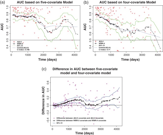
We now illustrate the proposed methods using data from 312 randomized subjects from the Mayo primary biliary cirrhosis (PBC) study, a randomized, placebo-controlled trial of the drug D-penicillamine (DPCA) for the treatment of PBC conducted at the Mayo clinic between 1974 and 1984 (Fleming and Harrington 1991). Among these subjects, 125 died by the end of the follow-up. We demonstrate AUC curves associated with four-covariate and five-covariate model, their difference and the associated point-wise 95% confidence interval.

We consider a score from Cox model with covariates: log(bilirubin), log(prothrombin time), edema, albumin, and age. The log hazard ratios under PH assumption can be found in Heagerty and Zheng (2005, Table 3). The prognostic score from this model has been used previously (Costa and Shaw 2009; Fleming and Harrington 1991). Here, we address the question: how well does this score discriminate between subjects who are at risk of an imminent failure from those who are not. We plot the WMR curve and associated point-wise 95% confidence interval (Figure 1(a)). A bandwidth of 504 days was used such that the IMSE is minimized (h = 0.8). Another WMR curve based on a four-covariate model (bandwidth = 504 days) (log(prothrombin time), edema, albumin, and age) with point-wise 95% confidence interval is plotted in Figure 1(b). This modified Mayo score is less predictive than the score from the five-covariate model and the time-specific accuracy decreases steadily over time. We further compared the predictive accuracy of the five-covariate and four-covariate model scores using the difference in the respective WMR curves. We plotted the difference in the WMRs in Figure 2 along with the point-wise 95% confidence interval for the difference using the proposed variance estimator of the dWMR(t) (see Section 3). Throughout the entire time period considered here, the predictive accuracy of the five-covariate model is generally better than the four-covariate model.

Figure 1.

(a) and (b) The WMR curve and point-wise confidence interval for Mayo PBC data (bandwidth = 504 days). (c) The dWMR curve for the difference in AUC from five-covariate and four-covariate models and point-wise confidence interval for Mayo PBC data (bandwidth = 504 days). (a) Five-covariate model. (b) Four-covariate model. (c) Difference between five- and four-covariate models.

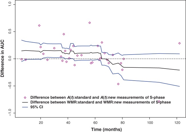
Figure 2.

The dWMR curve for the difference between AUC (solid, middle line) from the new and standard percent S-phase measurements and point-wise confidence interval (solid, top and bottom lines) among young-onset breast cancer patients. The raw differences are indicated by diamonds.

In Figure 1(a), we show the proposed estimator, and show the result of using a simple LOWESS smoother (solid, blue line) that tends to dampen the fluctuation observed after 2000 days. We do not have any biological explanation for the late increase, and expect this to likely reflect variability and/or be the result of cross-validation choosing a relatively small bandwidth. One additional analysis that could explain the observed pattern would be to consider bandwidth estimation based on IMSE separately over the first 2000 days and the later times—this would likely allow a larger bandwidth at later times and therefore tend to smooth this part of the curve in more agreement with the LOWESS estimator. We have introduced IMSE as one objective method for choosing the bandwidth, but other options are worth consideration. Figure 1(b) uses a different composite marker (excludes bilirubin) and shows a similar yet dampened pattern after 2000 days. The WMR curves, dWMR curve and the associated confidence intervals based on leave-one-out cross-validation were very similar to those estimated without cross-validation.

5.2. Example 2

In the second example, we focus on comparison of a new pathology measurement with a standard one as predictors of mortality among young breast cancer patients. A cohort of young (onset before age 45) subjects had primary tumor samples analyzed for the percent of cells in the S-phase of the replication cycle. A standard measurement of S-phase (in %) was obtained in addition to a new measurement (in %) based exclusively on epithelial cells that were sorted using flow cytometry. Survival subsequent to disease diagnosis was recorded on n = 253 subjects with a median observed follow-up time of 62 months. A prior analysis of the data (Heagerty and others 2000) using cumulative events inferred that the new marker was only superior during the first 60 months. Our proposed WMR methods allow us to directly compare the riskset rank based on the standard measure versus the new measure to see whether improvement is obtained, and to see whether improvement is uniform across time. Figure 2 shows the difference in the WMR as a function of time and clearly shows an advantage for the new marker but only during the first 60 months where cases ranked using the new measurement had an average percentile that was 12% higher. Thus, the use of the new graphical method allows a direct evaluation of both how much of an improvement is obtained, and of when improvement is obtained.

6. Discussion

In this article, we introduce a non-parametric estimator of a time-dependent predictive accuracy function that is useful for characterizing the accuracy of a predictive score or scalar marker for a survival time that may be censored. For the entire study duration, we look at the ability of the score to discriminate between subjects who are at risk of an impending failure (incident cases) from those who are not (dynamic controls). We use AUC(t) as a measure of predictive accuracy at t and show that a non-parametric estimator of AUC, namely the locally weighted average of the proportion of concordant case–control pairs, can be used to estimate this time-dependent concordance. The proposed estimator, WMR at t, is a smoothed version of time-specific AUCs within a neighborhood around each t and is similar to other smoothing approaches, yet is based on local U-statistic summaries. Furthermore, we showed that under certain conditions on the size of the control set when compared with the number of failures, the standardized estimator WMR(t) asymptotically follows a normal distribution. We provide an estimator of the asymptotic variance. Both the estimator and the variance can be easily estimated. We examined the estimator WMR(t) and the variance estimator via simulation studies and showed that both perform satisfactorily under realistic censoring proportions. We introduced a simple approach for comparing the predictive accuracy of two correlated markers using the difference in the respective WMR estimates. We proposed a variance estimator for this difference and evaluated the properties of the estimator via simulation. We applied the methods to the well-known Mayo PBC dataset, and compared the results with a semi-parametric estimator and drew similar conclusions.

For any given time point t, construction of a confidence interval for WMR(t) is straight-forward using the asymptotic properties presented here. In many applications, however, it may be desirable to obtain simultaneous confidence bands for the function WMR(t), so that a single probability statement can be made regarding the predictive accuracy curve over the entire time span of interest. While estimation of simultaneous confidence band (e.g. for cumulative hazard, survival curve, etc.) has received a wide attention in the survival analysis literature (Hall and Wellner 1980; Parzen and others 1997), the associated theory may not be applicable in our case (since the limiting process of WMR(⋅) may not possess an independent increment structure). When an estimator in such situations does not possess independent incremental structure, a well-known approach is to simulate a Gaussian process while keeping the observations fixed to approximate the distribution of the process and to estimate the appropriate quantiles based on the perturbed distribution. This approach has been used in the literature for the estimation of subject-specific cumulative hazard and survival function (Lin and others 1994), the difference in two survival functions (Parzen and others 1997), and contrast in two hazard functions (Gilbert and others 2002) and may be applicable for the estimation of simultaneous confidence bands for the WMR curve. Computationally simpler Bonferroni-type bands may also be useful in our setting. A third approach, stemming from literature on kernel smoothing (Wu and others 1998), first establishes simultaneous confidence intervals for a set of grid points and then bridges the gap between the grid points via smoothness conditions of the curve. However, additional careful work is needed to extend simultaneous methods to our application and is an important direction for future research.

For the basic development, we assume that the censoring time, C_i, is independent of the survival time, T_i. Estimation that allows this assumption to be relaxed to permit the weaker assumption of conditional independence between the failure and censoring times given the marker would be appropriate in certain settings and therefore warrants further development.

7. Acknowledgments

Conflict of Interest: None declared.

8. Funding

This research was supported in part by the Intramural Research Program of the NIH, National Institute of Environmental Health Sciences (PSC) and by grants R01 HL072966 and U54 RR024379.

Appendix A

A.1. Asymptotic Normality of WMR

Suppose that we are interested in characterizing the predictive accuracy of the marker at t using , where . We assume that denotes the unique failure times with . We first assume that no subjects were censored in (s_Lt+1,s_Lt+mt) and the subjects surviving s_Lt+mt are considered censored at s_Lt+mt, so that the event times of these subjects cannot be ordered.

We first restate the following theorem from Lee (1990).

Theorem A1 —

Let be a weighted U-statistic of order k = 2 and define

Suppose that the following conditions hold when :

1. 
2. 

3. for some δ>0.

Then .

Here ψ_i(x) = E(ψ(X_i,X_j)|X_i = x) is the conditional expectation given X_i = x.

For asymptotic normality of WMR, consider X = (T,M*) = (T, − M). We define a U-statistic with event time T and a baseline marker M* as

where R_i is the rank of the marker value M* for a subject a(i) who experienced the ith ordered failure: T_a(i) = s_i. Also

Note that, the event times T_l1,T_l2 for two subjects surviving past s_Lt+mt cannot be ordered; we assume that sgn(l₁ − l₂) = 0 for those subjects. Finally, we assume that the weights are as follows:

if s_i and s_j can be ordered and w_ij = 0 when the event times s_i and s_j cannot be ordered. We now state the asymptotic normality of WMR as in the following theorem.

Theorem A2 —

Suppose when , where n − (L_t+m_t) denotes the number of subjects surviving past t_(Lt+mt) or equivalently, surviving past t+h_n and let , . Then

where V_n = var[WMR_n(t)] and b_n(t) denotes the bias: E[WMR_n(t)] = AUC(t) + b_n(t).

Proof —

To prove the asymptotic normality of WMR(t), we note that WMR and simply verify conditions (i)–(iii).

Note that the assumption (iii) holds for ψ(X_i,X_j) = sgn(i − j) sgn(R_i − R_j) since |ψ(X_i,X_j)|≤1.

Dropping subscript n from w_i,n to simplify the notation, we see

so that

where . Also,

Thus, condition (i) is satisfied. If subjects were censored between s_Lt+1 and s_Lt+mt, the inequality above will still hold. Finally,

and hence condition (ii) is also satisfied (whether subjects were censored between s_Lt+1 and s_Lt+mt) if as .

Appendix B

B.1. Variance of WMR

As before, we want to characterize the predictive accuracy of the marker at t using , where . Suppose, . Note that

where

The variance is the same as the variance of an AUC estimator using the proportion of concordant case–control pairs as obtained from a case-control study (Pepe 2003). When there are d_t events at t,

where

However, the expression for cov{A(t),A(s)} remains the same.

To estimate the variance, we use the empirical normal quantiles of the rank of the markers instead of the markers themselves. Finally, the quantities of interest are estimated assuming normality of the transformed marker:

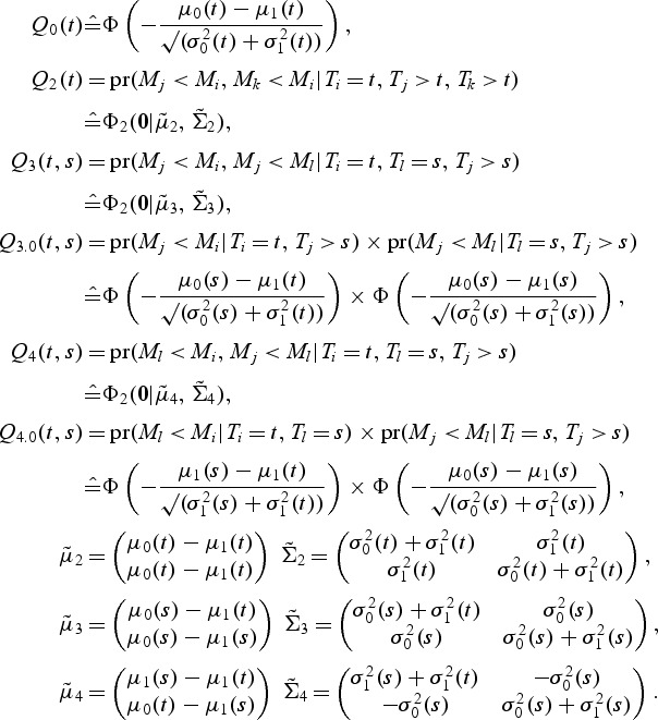If there are more than one case at t, μ₁(t) and can be estimated as the mean and variance of the (transformed) marker of the cases at t, while μ₀(t) and are estimated as the mean and variance of the (transformed) marker of the controls at t. However, usually there is only a single incident event at t. Hence, we assume that the mean marker values for the cases within the neighborhood of interest (or ) is constant: μ₁(t) = μ₁(s) and , and use all the cases within the neighborhood to estimate μ₁(t) and .

References

- Antolini L., Boracchi P., Biganzoli E. A time-dependent discrimination index for survival data. Statistics in Medicine. 2005;24:3927–3944. doi: 10.1002/sim.2427. [DOI] [PubMed] [Google Scholar]
- Coombes J. M., Trotter J. F. Development of the allocation system for deceased donor liver transplantation. Clinical Medicine and Research. 2005;3:87–92. doi: 10.3121/cmr.3.2.87. [DOI] [PMC free article] [PubMed] [Google Scholar]
- Costa M. J., Shaw J. E. H. Parametrization and penalties in spline models with an application to survival analysis. Computational Statistics and Data Analysis. 2009;53:657–670. [Google Scholar]
- Fleming T. R., Harrington D. P. Counting Process and Survival Analysis. New York: John Wiley & Sons; 1991. [Google Scholar]
- Gilbert P. B., Wei L. J., Kosorok M. R., Clemens J. D. Simultaneous inferences on the contrast of two hazard functions with censored observations. Biometrics. 2002;58:773–780. doi: 10.1111/j.0006-341x.2002.00773.x. [DOI] [PubMed] [Google Scholar]
- Gonen M., Heller G. Concordance probability and discriminatory power in proportional hazards regression. Biometrika. 2005;92:965–970. [Google Scholar]
- Gries C. J., Rue T. C., Heagerty P. J., Edelman J. D., Mulligan M. S., Goss C. Development of a predictive model for long-term survival after lung transplantation and implications for the lung allocation score. Journal of Heart Lung Transplant. 2010;29:731–738. doi: 10.1016/j.healun.2010.02.007. H. [DOI] [PMC free article] [PubMed] [Google Scholar]
- Hall W. J., Wellner J. A. Confidence bands for a survival curve from censored data. Biometrika. 1980;67:133–143. [Google Scholar]
- Hardle W. Applied Nonparametric Regression. Cambridge: Cambridge University Press; 1992. [Google Scholar]
- Harrell F. E., Califf R. M., Pryor D. B., Lee K. L., Rosati R. A. Evaluating the yield of medical tests. Journal of the American Medical Association. 1982;247:2543–2546. [PubMed] [Google Scholar]
- Heagerty P. J., Lumley T., Pepe M. S. Time-dependent ROC curves for censored survival data and a diagnostic marker. Biometrics. 2000;56:337–344. doi: 10.1111/j.0006-341x.2000.00337.x. [DOI] [PubMed] [Google Scholar]
- Heagerty P. J., Zheng Y. Survival model predictive accuracy and ROC curves. Biometrics. 2005;61:92–105. doi: 10.1111/j.0006-341X.2005.030814.x. [DOI] [PubMed] [Google Scholar]
- Lee A. J. U-statistics: Theory and Practice. New York: Marcel Dekker; 1990. [Google Scholar]
- Lin D. Y., Fleming T. R., Wei L. J. Confidence bands for survival curves under the proportional hazards model. Biometrika. 1994;81:73–81. [Google Scholar]
- Parzen M. I., Wei L. J., Ying Z. Simultaneous confidence intervals for the difference of two survival functions. Scandanavian Journal of Statistics. 1997;24:309–314. [Google Scholar]
- Pepe M. S. The Statistical Evaluation of Medical Tests for Classification and Prediction. Oxford: Oxford University Press; 2003. [Google Scholar]
- Wu C. O., Chiang C.-T., Hoover D. R. Asymptotic confidence regions for kernel smoothing of a varying-coefficient model with longitudinal data. Journal of the American Statistical Association. 1998;93:1388–1402. [Google Scholar]