Fast ℓ₁-SPIRiT Compressed Sensing Parallel Imaging MRI: Scalable Parallel Implementation and Clinically Feasible Runtime

Abstract

We present ℓ₁-SPIRiT, a simple algorithm for auto calibrating parallel imaging (acPI) and compressed sensing (CS) that permits an efficient implementation with clinically-feasible runtimes. We propose a CS objective function that minimizes cross-channel joint sparsity in the Wavelet domain. Our reconstruction minimizes this objective via iterative soft-thresholding, and integrates naturally with iterative Self-Consistent Parallel Imaging (SPIRiT). Like many iterative MRI reconstructions, ℓ₁-SPIRiT’s image quality comes at a high computational cost. Excessively long runtimes are a barrier to the clinical use of any reconstruction approach, and thus we discuss our approach to efficiently parallelizing ℓ₁-SPIRiT and to achieving clinically-feasible runtimes. We present parallelizations of ℓ₁-SPIRiT for both multi-GPU systems and multi-core CPUs, and discuss the software optimization and parallelization decisions made in our implementation. The performance of these alternatives depends on the processor architecture, the size of the image matrix, and the number of parallel imaging channels. Fundamentally, achieving fast runtime requires the correct trade-off between cache usage and parallelization overheads. We demonstrate image quality via a case from our clinical experimentation, using a custom 3DFT Spoiled Gradient Echo (SPGR) sequence with up to 8× acceleration via poisson-disc undersampling in the two phase-encoded directions.

1 Introduction

Imaging speed is a major limitation of MR Imaging, especially in comparison to competing imaging modalities such as Computed Tomography (CT). MR allows much more flexible contrast-generation and does not expose patients to ionizing radiation, and hence does not increase risk of cancer. However, other imaging modalities are substantially more popular, as MR scans are slow, expensive, and in some cases less robust. Patient motion during long scans frequently causes image artifacts, and for uncooperative patients, like children, anesthesia is a frequent solution. Acquisition time in MRI can be reduced by faster scanning or by subsampling. Parallel imaging [31, 29, 14] is a well-established acceleration technique based on the spatial sensitivity of array receivers. Compressed sensing (CS) [7, 10, 21] is an emerging acceleration technique that is based on the compressibility of medical images. Attempts to combine the two have mostly focussed on extensions of iterative SENSE [28] with SparseMRI [21]. In [4] Block et al., added total-variation to a SENSE reconstruction from radial sampling, Liang et al., in [19] showed improved acceleration by first performing CS on aliased images and then applying SENSE to unfold the aliasing, Otazo et al. used compressed sensing with SENSE to accelerate first-pass cardiac perfusion [27]. More recently [34, 39] have presented some improvements, again, using an extension of SENSE. The difficulty in estimating exact sensitivity maps in SENSE has created the need for autocalibrating techniques. One class of autocalibrating algorithms extends the SENSE model to joint estimation of the images and the sensitivity maps [41, 35]. Combination of these approaches with compressed sensing have also been proposed. Knoll et al. [17] proposed a combination with Uecker’s non-linear inversion and Huang et al. [15] proposed a self-feeding SENSE combined with compressed sensing.

A different, yet very popular class of autocalibrating techniques are methods like GRAPPA [14] that do not use the sensitivity maps explicitly. In [22] we proposed an optimized iterative method, SPIRiT, and demonstrated the combination with non-linear regularization. In [20] we presented and extension, ℓ₁-SPIRiT, that synergistically combines SPIRiT with compressed sensing and in [38, 37] we presented more details and clinical results in pediatric patients.

The combination of compressed sensing with parallel imaging has the advantage of improved image quality, however it comes at a cost. These algorithms involve substantially more computation than direct or iterative linear reconstructions.

In this paper we discuss the ℓ₁-SPIRiT reconstruction. ℓ₁-SPIRiT solves a constrained non-linear optimization over the image matrix. The non-linearity of this optimization necessitates an iterative reconstruction, and we describe our simple and efficient POCS algorithm in Secion 3.

A recent trend in MRI has been to accelerate reconstructions by implementing and optimizing them for massively parallel processors. Silicon manufacturing technology has recently experienced the end of a trend that produced the incredible pace of comptuational speed during the 1990’s [12]. In the past decade, all major microprocessor vendors have increased the computational throughput of their designs by introducing programmer-visible parallelism. Intel and AMD provide 4–16 CPU cores per socket, and GPGPUs typically have 16–32 massively multithreaded vector cores per socket. In each case, the computational throughput of the processor is proportional to the number of cores, and future designs will have larger numbers of cores.

This paper discusses the massively parallel implementation of ℓ₁-SPIRiT on these processors. The resulting sub-minute runtimes demonstrate that computational expense is not a substantial obstacle to clinical deployment of ℓ1-SPIRiT. Many previous works have demonstrated substantial improvement in reconstruction runtime using GPUs and multi-core CPUs as parallel execution platforms. Chang and Ji [8] demonstrated multi-channel acceleration by solving SparseMRI reconstruction separately for each channel and reporting 1.6–2.0 acceleration using 4 cores. More recently Kim et al. [16] present a high-performance implementation of a SENSE based compressive sensing recosntruction, describing many low-level optimizations that apply for both CPU and GPU architectures.

Stone et al. [33] describe the implementation of an iterative reconstruction using the Conjugate Gradient (CG) algorithm to solve regularized linear reconstructions for non-cartesian trajectories. Their implementation relies on a highly optimized GPU implementation of a non-uniform Fourier transform (NDFT) to perform sub-minute noncartesian reconstructions. Wu et al. [40, 43] have generalized this work to model other acquisition effects in the NDFT, such as off-resonance and sensitivity encoding. Several other works have discussed the GPU implementation of Gridding [3], a highly accurate NDFT approximation. Gregerson [13] discusses the performace trade-offs of different parallelization strategies for the gridding interpolation. Obeid et al [26] use a spatial-partitiong approach to optimize gridding interpolation, and reporting 1–30 second runtimes. Nam et al. [1] describe another gridding implementation achieving sub-second interpolations for highly undersampled data. Several other works have presented GPU implementations of Parallel Imaging (PI) reconstructions with clinically-feasible runtimes. Roujol et al. [30] describe GPU implementation of temporal sensitivity encoding (TSENSE) for 2D interventional imaging. Sorenson et al. [32] present a fast iterative SENSE implementation which performs 2D gridding on GPUs. Uecker [36] describes a GPU implementation of a non-linear approach to estimate PI coil sensitivity maps during image reconstruction.

This work presents the parallelization of an autocalibrating approach, ℓ1-SPIRiT, via multi-core CPUs and GPUs and the resulting clinically-feasible reconstruction runtimes. Moreover we discuss the approach taken to parallelizing the various operations within our reconstruction, and the performance trade-offs in different parallelization strategies. Additionally, we discuss the data-size dependence of performance-relevant implementation decisions. To our knowledge, no previous works have addressed this issue.

2 iTerative Self-Consistent Parallel Imaging Reconstruction (SPIRiT)

SPIRiT is a coil-by-coil autocalibrating parallel imaging method and is described in detail in [22]. SPIRiT is similar to the GRAPPA parallel imaging method in that it uses autocalibration lines to find linear weights to synthesize missing k-space. The SPIRiT model is based on self-consistency of the reconstructed data with the acquired k-space data and with the calibration.

SPIRiT is an iterative algorithm in which in each iteration non-acquired k-space values are estimated by performing a linear combination of nearby k-space values. The linear combination is performed using both acquired k-space samples as well as estimated values (from the previous iteration) for the non-acquired samples. If we denote x_i as the entire k-space grid of the i^th coil, then the consistency criterion has a form of a series of convolutions with the so called SPIRiT kernels g_ij. The SPIRiT kernels are obtained by calibration from auto calibration lines similarly to GRAPPA. If N_c is the total number of channels, the calibration consistency criterion can be written as

$$x_i=\sum _{j=1}^{Nc}{g}_{ij}\otimes x_j.$$

The SPIRiT calibration consistency for all channels can be simply written in matrix form as

$$x=Gx,$$

where x is a vector containing the concatenated multi-coil data and G is an aggregated operator that performs the appropriate convolutions with the g_ij kernels and the appropriate summations. As discussed in [22], the G operator can be implanted as a convolution in k-space or as multiplication in image space.

In addition to consistency with the calibration, the reconstruction must also be consistent with the acquired data Y. This can be simply written as

$$y=Dx,$$

where D is an operator that select the acquired k-space out of the entire k-space grid. In [22] two methods were proposed to find the solution that satisfies the constraints. Here we would like to point out the projection over convex sets (POCS) approach which uses alternate projections that enforce the data consistency and calibration consistency. In this paper we extend the POCS approach to include sparsity constraints for combination with compressed sensing.

As previously mentioned, the convolution kernels g_i,j are obtained via a calibration from the densely sampled auto-calibration region in the center of k-space, commonly referred to as the Auto-Calibration Signal or ACS lines. In the reconstruction we would like to find x that satisfies x = Gx. However in the calibration x is known and G is unknown. We can therefore solve for the g_ij’s by reformatting the data x appropriately and solving a series of least-squares problems to calibrate g_ij. This procedure is similar to calibrating GRAPPA kernels.

3 ℓ₁-SPIRiT Reconstruction

Variations of the ℓ1-SPIRiT reconstruction have been mentioned in several conference proceedings [20, 24, 18, 38]. More detailed descriptions are given in [22] and in [37]. But for the sake of completeness and clarity we include here a detailed description of the variant that is used in this paper.

ℓ1-SPIRiT is an approach for accelerated sampling and reconstruction that synergistically unifies compressive sensing with auto-calibrating Parallel imaging. The sampling is optimized to provide the incoherence that is required for compressed sensing yet compatible to parallel imaging. The reconstruction is an extension of the original SPIRiT algorithm that in addition to enforcing consistency constraints with the calibration and acquired data, enforces joint-sparsity of the coil images in the Wavelet domain. Let y be a the vector of acquired k-space measurements from all the coils, F a Fourier operator applied individually on each coil-data, D a subsampling operator that chooses only acquired k-space data out of the entire k-space grid, G an image-space SPIRiT operator that was obtained from auto-calibration lines, Ψ a wavelet transform that operates on each individual coil separately. ℓ₁-SPIRiT solves for the multi-coil images concatenated into the vector x which minimizes the following problem:

$${\text{minimize}}_x\text{Joint}{\ell }_1(\mathbf{\Psi }x)$$ (1)

$$\text{subject}\text{to}\mathbf{DF}x=y$$ (2)

$$\mathbf{G}x=x$$ (3)

The function Joint ℓ₁(·) is a joint ℓ₁-ℓ₂-norms convex functional and is described later in more detail. Minimizing the objective (1) enforces joint sparsity of wavelet co-efficients between the coils. The constraint in (2), is a linear data-consistency constraint and in (3) is the SPIRiT parallel imaging consistency constraint. The Wavelet transform [5] Ψ is well-known to sparsify natural images, and thus used frequently in Compressive Sensing applications as a sparsifying basis. Just as the Fourier transform, it is a linear operation that can be computed via a fast O(n log n) algorithm.

As previously mentioned, in this work we solve the above problem via a an efficient POCS algorithm, shown in Figure 1. The POCS algorithm converges to a fixed-point that satisfies the above constraints, often within 50–100 iterations.

Figure 1.

The POCS algorithm. Line (A) performs SPIRiT k-space interpolation, implemented as voxel-wise matrix-vector multiplications in the image domain. Line (B) performs Wavelet Soft-thresholding, computationally dominated by the forward/inverse Wavelet transforms. Line (C) performs the k-space consistency projection, dominated by inverse/forward Fourier transforms.

3.1 Joint-Sparsity of Multiple Coils

We perform soft-thresholding on the Wavelet coefficients to minimize the ℓ1-objective function (1). The soft-thresholding function (x) is defined element-wise for x ∈ as:

$${\mathcal{S}}_{\lambda }(x)=\frac{x}{\mid x\mid }·max(0,\mid x\mid -\lambda )$$

where |x| is the complex modulus of x. The parameter λ estimates the amplitude of noise and aliasing in the Wavelet basis, and the soft-thresholding operation is a well-understood component of many denoising [11] and compressive sensing algorithms [9].

The individual coil images are sensitivity weighted images of the original image of the magnetization. Edges in these images appear in the same spatial position, and therefore coefficients of sparse transforms, such as wavelets, exhibit similar sparsity patterns. To exploit this, we use a joint-sparsity model. In compressed sensing, sparsity is enforced by minimizing the ℓ₁-norm of a transformed image. The usual definition of the ℓ₁-norm is the sum of absolute values of all the transform coefficients, ${\sum }_c{\sum }_r\mid w_{cr}\mid ={\sum }_c{\sum }_r\sqrt{{\mid w_{rc}\mid }^2}$, where c is the coil index and r is the spatial index. In a joint-sparsity model we would like to jointly penalize coefficients from different coils that are at the same spatial position. Therefore we define a joint ℓ₁ as:

$$\text{Joint}{\ell }_1(w)=\sum _r\sqrt{\sum _c{\mid w_{rc}\mid }^2}$$

In a joint ℓ₁-norm model, the existence of large coefficient in one of the coils, protects the coefficients in the rest of the coils from being suppressed by the non-linear reconstruction. In the POCS algorithm joint sparsity is enforces by soft-thresholding the magnitude of the wavelet coefficients across coils, at a particular position.

3.2 Computational Complexity

If n_c is the number of PI channels and v is the number of voxels per PI channel, the computational complexity of our algorithm is:

$$O(C_C·n_c^3+T·((C_W+C_F)·n_c\mathit{v}logv+C_S·n_c^{2}v))$$

T is the number of iterations the POCS algorithm performs. The algorithm often converges with sufficient accuracy within 50–100 iterations. The constants C_W, C_F, C_S, and C_C indicate that the relative computational cost of the Wavelet transforms, Fourier transforms, and SPIRiT interpolation and calibration are heavily dependent on input data size. Section 6 presents more detailed runtime data.

The $n_c^3$ term represents the SPIRiT calibration, which performs a least-norm least-squares fit of the SPIRiT model to a densely sampled autocalibration region in the center of k-space. Solving each of these systems independently leads to an $O(n_c^4)$ algorithm, which is prohibitively expensive for large coil arrays. However, the n_c linear systems are very closely related and can be solved efficiently with only a single Cholesky decomposition of a square matrix of order O(n_c), hence the $O(n_c^3)$ complexity of our method. See Appendix A for a complete derivation of the algorithm. This derivation can potentially be used to accelerate the computation of GRAPPA kernels as well.

The n_cv log v term represents the Fourier and Wavelet transforms, and the $n_c^{2}v$ term represents the image-domain implementation of the k-space SPIRiT interpolation. This k-space convolution is implemented as multiplication in the image domain, hence the linearity in v of this term. Due to the $O(n_c^{2}v)$ complexity, SPIRiT interpolation is asymptotically the bottleneck of the POCS algorithm. All other operations are linear in the number of PI channels, and at worse log-linear in the number of voxels per channel. There are several proposed approaches that potentially reduce the complexity of the SPIRiT interpolation without degrading image quality. For example ESPIRiT [18] performs an eigen decomposition of the G matrix, and uses a rank-one approximation during POCS iterations. Also, coil array Compression [6, 42] can reduce the number of parallel imaging channels to a small constant number of virtual channels. Our software includes implementations of both of these approaches, and in practice the ℓ1-SPIRiT solver is rarely run with more than 8 channels.

One could solve the ℓ₁-SPIRiT reconstruction problem (Eqns 1–3) via an algorithm other than our POCS approach, for example non-linear Conjugate Gradients (NLCG). The computational complexity of alternate algorithmic approaches would differ only in constant factors. The same set of computations would still dominate runtime, but a different number of iterations would be performed and potentially a different number of these operations would be computed per iteration. End-to-end reconstruction times would differ, but much of the performance analysis in this work applies equally well to alternate algorithmic approaches.

4 Fast Implementation

The POCS algorithm is efficient: in practice, it converges rapidly and performs a minimal number of operations per iteration. Still, a massively parallel and well-optimized implementation is necessary to achieve clinically feasible runtimes. A sequential C++ implementation runs in about 10 minutes for the smallest reconstructions we discuss in this paper, and in about 3 hours for the largest. For clinical use, images must be available immediately after the scan completes in order to inform the next scan to be prescribed. Moreover, time with a patient in a scanner is limited and expensive: reconstructions requiring more than a few minutes of runtime are infeasible for on-line use.

In this section, we discuss the aspects of our reconstruction implementation pertinent to computational performance. While previous works have demonstrated the suitability of parallel processing for accelerating MRI reconstructions, we provide a more didactic and generalizable description intended to guide the implementation of other reconstructions as well as to explain our implementation choices.

4.1 Parallel Processors

Many of the concerns regarding efficient parallel implementation of MRI reconstructions are applicable to both CPU and GPU architectures. These two classes of systems are programmed using different languages and tools, however have much in common. Figure 2 establishes a four-level hierarchy that one can use to discuss parallelization decisions. In general, synchronization is more expensive and aggregate data access bandwidth is less at “higher” levels of the hierarchy (i.e. towards the top of Figure 2). For example, Cuda GPGPUs can synchronize threads within a core via a syncthreads() instruction at a cost of a few processor cycles, but synchronizing all threads within a GPU requires ending a grid launch at a cost of ≈ 5 μs, or 7,500 cycles. CPU systems provide less elaborate hardware-level support for synchronization of parallel programs, but synchronization costs are similar at the corresponding levels of the processor hierarchy. On CPUs, programs synchronize via software barriers and task queues implemented on top of lightweight memory-system support. With respect to data access, typical systems have ≈ 10 TB/s (10¹³ bytes/s) aggregate register-file bandwidth, but only ≈ 100 GB/s (10¹¹ bytes/s) aggregate DRAM bandwidth. Exploiting locality and data re-use is crucial to performance.

Figure 2.

The four-level hierarchy of modern parallel systems. Nodes contain disjoint DRAM address spaces, and communicate over a message-passing network in the CPU case, or over a shared PCI-Express network in the GPU case. Sockets within a node (only one shown) share DRAM but have private caches – the L3 cache in CPU systems and the L2 cache in Fermi-class systems. Similarly Cores share access to the Socket-level cache, but have private caches (CPU L2, GPU L1/scratchpad). Vector-style parallelism within a core is leveraged via Lanes – SSE-style SIMD instructions on CPUs, or the SIMT-style execution of GPUs.

In this work, we do not further discuss cluster-scale parallelization (among Nodes in Figure 2). The CPU parallelization we’ll describe in this section only leverages the parallelism among the multiple Sockets/Cores a single Node. As indicated by Figure 2, parallelization decisions at this level are analogous to decisions among the multiple GPUs in a single system, but we leave more detailed performance analysis of cluster-parallelization to future work.

4.2 Data-Parallelism and Geometric Decomposition

The computationally intense operations in MRI reconstructions contain nested data parallelism. In particular, operations such as Fourier and Wavelet transforms are performed over k-dimensional slices through the N-dimensional reconstruction volume, with k < N. In most cases the operations are performed for all k-dimensional (k-D) slices, providing another source of parallelism to be exploited for accelerating the reconstruction. The k-D operations themselves are parallelizable, but usually involve substantial synchronization and data-sharing. Whenever possible, it is very efficient to exploit this additional level of parallelism. For the purposes of software optimization, the size and shape of the N-dimensional (N-D) data are important. The Geometric Decomposition (GD) design pattern [23] discusses the design of parallel programs in which the data involved have geometric structure. GD suggests the parallelization should follow a division of the data that follows this structure, in order to achieve good caching and inter-thread communication behavior.

Recall from Figure 2 that modern processor architectures provide four levels at which to exploit parallelism. An efficient parallel implementation must decide at which levels of the processor hierarchy to exploit the levels of the nested parallelism in MRI reconstruction.

In volumetric MRI reconstructions, all of these operations are applied to the 4-D array representing the multi-channel 3D images. Figure 3 illustrates that the exploitable parallelism of operations over these arrays is two-level: operations like Fourier and Wavelet transforms applied to the individual channels’ images exhibit massive voxel-wise parallelism and require frequent synchronization; but the transforms of the 4–32 channels can be performed independently and in parallel.

Figure 3.

Hierarchical sources of parallelism in 3D MRI Reconstructions. For general reconstructions, operations are parallelizable both over channels and over image voxels. If there is a fully-sampled direction, for example the readout direction in Cartesian acquisitions, then decoupling along this dimension allows additional parallelization.

In cartesian acquisisions, the readout direction is never undersampled. Similarly in stack-of-spirals or stack-of-radial acquisitions, the same non-cartesian sampling of x − y slices is used for every z position. In these cases, the 3D reconstruction can be decoupled into independent 2D reconstructions for each undersampled slice. Parallelizing over independent 2D reconstructions is very efficient, as the decoupled 2D reconstructions require no synchronization. Our Cuda ℓ₁-SPIRiT solver is able to run multiple 2D problems simultaneously per GPU in batch mode. Large batch sizes require more GPU memory, but expose more parallelism and can more effectively utilize the GPU’s compute resources.

4.3 Size-Dependence and Cache/Synchronization Trade-off

One can produce several functionally equivalent implementations by parallelizing at different levels of the hierarchy in Figure 2. These different implementations will produce identical results¹, but have very different performance characteristics. Moreover, the performance of a given implementation may differ substantially for different image matrix sizes and coil array sizes. In general, the optimal implementation is a trade-off between effective use of the cache/memory hierarchy and amortization of parallelization overheads.

For example, one may choose to exploit the voxel-wise parallelism in an operation only among the vector lanes within a single processor core. The implementation can then exploit parallelism over multiple channels and 2D slices over the multiple cores, sockets, and nodes in the system. Utilizing this additional parallelism will increase the memory footprint of the algorithm, as the working set of many 2D slices must be resident simultaneously. This consideration is particularly important for GPU systems which have substantially less DRAM capacity than CPU systems.

On the other hand, one may leverage voxel-wise parallelism among the multiple cores within a socket, the multiple sockets within the system, or among the multiple nodes. In doing so the implementation is able to exploit a larger slice of the system’s processing and memory-system resources while simultaneously reducing memory footprint and working-set size. The favorable caching behavior of the smaller working set may result in a more efficient implementation. However it is more expensive to synchronize the higher levels of the processing hierarchy. Furthermore for problems with smaller matrix sizes, voxel-wise parallelism may be insufficient to fully saturate the processing resources at higher levels. Even when caching behavior is more favorable, this over-subscription of resources may degrade performance.

Which implementation provides better performance depends both on the size of the input data and on the size of the processor system. When the image matrix is very high-resolution (i.e. has a large number of voxels) or the processing system is relatively small (i.e. a small number of processor cores), then one can expect a high degree of efficiency from exploiting voxel-wise parallelism at higher levels of the hierarchy. If the image matrix is relatively small or the processor system is very large, then one should expect that parallelism from the Channel and Decoupled-2D levels of Figure 3 is more important. As the number of processing cores per system and the amount of cache per core both continue to increase over time, we expect the latter case to become more common in the future.

4.4 Parallel Implementation of ℓ₁-SPIRiT

In the case of ℓ₁-SPIRiT, there are four operations which dominate runtime: SPIRiT auto-calibration, Fourier transforms during the k-space consistency projection, Wavelet transforms during the joing soft-thresholding, and the image-domain implementation of SPIRiT interpolation. Figure 4 depicts the overall flow of the iterative reconstruction. Note that PI calibration must be performed only once per reconstruction, and is not part of the iterative loop.

Figure 4.

(a) Flowchart of the ℓ₁-SPIRiT POCS algorithm and the (b) SPIRiT, (c) Wavelet joint-threshold and (d) data-consistency projections

SPIRiT Auto-Calibration

Our ℓ₁-SPIRiT implementation performs auto-calibration by fitting the SPIRiT consistency model to the densely sampled Auto-Calibration Signal (ACS), which requires solving a least-squares least-norm problem for each PI channel. Note that while we perform the POCS iterations over decoupled 2D slices, we perform calibration in full 3D. The SPIRiT interpolation kernels for the 2D problems are computed via an inverse Fourier transform in the readout direction.

As discussed in Appendix A, the auto-calibration is computationaly dominated by two operations: the computation of a rank-k matrix product A^*A and a Cholesky factorization A = LL^*, which itself is dominated by rank-k products. Numerical linear algebra libraries for both CPUs and GPUs are parallelized via an output-driven scheme that requires very little inter-thread synchronization. For example, when computing a matrix-matrix product C = AB each element c_i,j is computed as an inner product of a row aⁱ of A with a column b_j of B. All such products can be computed independently in parallel, and are typically blocked to ensure favorable cache behavior.

The SPIRiT Operator in Image Space

Figure 4 (b) illustrates the image-domain implementation of SPIRiT interpolation Gx. Gx computes a matrix-vector multiplication per voxel – the length n_c (# PI channels) vector is composed of the voxels at a given location in all PI channels. For efficiency in the Wavelet and Fourier transforms, each channel must be stored contiguously – thus the cross-channel vector for each voxel is non-contiguous. Our implementation of the interpolation streams through each channel in unit-stride to obviate inefficient long-stride accesses or costly data permutation. The image-domain implementation is substantially more efficient than the k-space implementation, which performs convolution rather than a multiplication. However, the image-domain representation of the convolution kernels requires a substantially larger memory footprint, as the compact k-space kernels must be zero-padded to the image size and Fourier transformed. Since SPIRiT’s cross-coil interpolation is an all-to-all operation, there are $n_c^2$ such kernels. This limits the applicability of the image-domain SPIRiT interpolation when many large-coil-array 2D problems are in flight simultaneously. This limitation is more severe for the Cuda implementation than the OpenMP implementation, as GPUs typically have substantially less memory capacity than the host CPU system.

Enforcing Sparsity by Wavelet Thresholding

Figure 4 (c) illustrates Wavelet Soft-thresholding. Similarly to the Fourier transforms, the Wavelet transforms are performed independently and in parallel for each channel. Our Wavelet transform implementation is a multi-level decomposition via a separable Daubechies 4-tap filter. Each level of the decomposition performs low-pass and high-pass filtering of both the rows and columns of the image. The number of levels of decomposition performed depends on the data size: we continue the wavelet decomposition until the approximation coefficients are smaller than the densely sampled auto-calibration region. Our OpenMP implementation performs the transform of a single 2D image in a single OpenMP thread, and parallelizes over channels 2D slices.

We will present performance results for two alternate GPU implementations of the Wavelet transform. The first parallelizes a 2D transform over multiple cores of the GPU, while the second is parallelized only over the vector lanes within a single core. The former is a finer-grained parallelization with a small working set per core, and permits an optimization that greatly improves memory system performance. As multiple cores share the transform for a single 2D transform, the per-core working set fits into the small l1-cache of the GPU. Multiple Cuda thread blocks divide the work of the convolutions for each channel’s image, and explicitly block the working data into the GPU’s local store. Parallelism from multiple channels is exploited among multiple cores when a single 2D transform cannot saturate the entire GPU. The latter parallelization exploits all voxel-wise parallelism of a 2D transform within a single GPU core, and leverages the channel-wise and slice-wise parallelism across multiple cores. The working set of a single 2D image does not fit in the l1 cache of the GPU core and we cannot perform the explicit blocking performed in the previous case.

Enforcing k-space acquisition consistency

Figure 4 (d) illustrates the operations performed in the k-space consistency projection. The runtime of this computation is dominated by the forward and inverse Fourier transforms. As the FFTs are performed independently for each channel, there is n_c-way embarrassing parallelism in addition to the voxel-wise parallelism within the FFT of each channel. FFT libraries typically provide APIs to leverage the parallelism at either or both of these levels. The 2D FFTs of phase-encode slices in ℓ₁-SPIRiT are efficiently parallelized over one or a few processor cores, and FFT libraries can very effectively utilize voxel-wise parallelism over vector lanes. We will present performance results for the GPU using both the Plan2D API, which executes a single 2D FFT at a time, and the PlanMany API which potentially executes many 2D FFTs simultaneously. The latter approach more easily saturates the GPU’s compute resources, while the former approach is a more fine-grained parallelization with potentially more efficient cache-use.

5 Methods

Section 6 presents performance results for a representative sample of datasets from our clinical application. We present runtimes for a constant number of POCS iterations only, so the runtime depends only on the size of the input matrix. In particular, our reported runtimes do not depend on convergence rates or the amount of scan acceleration. We present performance results for six datasets, whose sizes are listed in Table 1.

Table 1.

Table of dataset sizes for which we present performance data. n_x is the length of a readout, n_y and n_z are the size of the image matrix in the phase-encoded dimensions, and n_c is the number of channels in the acquired data. Performance of SPIRiT is very sensitive to the number of channels, so we present runtimes for the raw 32-channel data as well as coil-compressed 8- and 16-channel data.

Dataset	nx	ny	nz	nc
A	192	256	58	8, 16, 32
B	192	256	102	8, 16, 32
C	192	256	152	8, 16, 32
D	192	256	190	8, 16, 32
E	320	260	250	8, 16, 32
F	320	232	252	8, 16, 32

We present several performance metrics of interest. First, we shall discuss the end-to-end runtime of our reconstruction to demonstrate the amount of wall-clock time the radiologist must wait from the end of the scan until the images are available. This includes the PI calibration, the POCS solver, and miscellaneous supporting operations. To avoid data-dependent performance differences due to differing convergence rates, we present runtime for a constant (50) number of POCS iterations.

To demonstrate the effectiveness of our O(n³) calibration algorithm, we compare its runtime to that of the “obvious” implementation which uses ACML’s implementation of the Lapack routine cposv to solve each coil’s calibration independently. The runtime of calibration does not depend on the final matrix size, but rather on the number of PI channels and the number of auto-calibration readouts. We present runtimes for calibrating 7 × 7 × 7 kernels averaged over a variety of ACS sizes.

We also present per-iteration runtime and execution profile of the POCS solver for several different parallelizations, including both CPU and GPU implementations. The per-iteration runtime does not depend on the readout length or the rate of convergence. Since we decouple along the readout dimension, POCS runtime is simply linear in n_x. Presenting per-iteration runtime allows direct comparison of the different performance bottlenecks of our multiple implementations.

Additionally, we explore the dependence of performance on data-size by comparing two alternate implementations parallelized for the GPU. The first exploits voxel-wise parallelism and channel-wise parallelism at the Socket-level from Figure 2, and does not exploit Decoupled-2D parallelism. This implementation primarily synchronizes via ending Cuda grid launches, incurring substantial overhead. However, the reduced working-set size increases the likelihood of favorable cache behavior, and enables further caching optimizations as described in Section 4.4 Fourier transforms are performed via the 2D API, which expresses a single parallel FFT per grid launch. Fermiclas GPUs are able to execute multiple grid launches simultaneously, thus this implementation expresses channel-wise parallelism as well. The second implementation exploits voxel-wise parallelism only within a core of the GPU, and maps the channel-wise and Decoupled-2D parallelism at the Socket-level. This implementation is able to use the more efficient within-core synchronization mechanisms, but has a larger working set per core and thus cannot as effectively exploit the GPU’s caches. It also launches more work simultaneously in each GPU grid launch than does the first implementation, and can more effectively amortize parallelization overheads. Fourier transforms are performed via the “Plan Many” API, which expresses the parallelism from all FFTs across all channels and all slices simultaneously.

All performance data shown were collected on our dual-socket × six-core Intel Xeon X5650 @2.67GHz system with four Nvidia GTX580s in PCI-Express slots. The system has 64GB of CPU DRAM, and 3GB of GPU DRAM per card (total 12 GB). We leverage Nvidia’s Cuda [25] extensions to C/C++ to leverage massively parallel GPGPU processors, and OpenMP ² to leverage multi-Core parallelism on the system’s CPUs. Additionally, multiple OpenMP threads are used to manage the interaction with the system’s multiple discrete GPUs in parallel. We leverage freely available high-performance libraries for standard operations: linear system solvers, matrix factorizations, Fourier transforms.

6 Performance Results

Figures 5–10 present performance data for our parallelized ℓ₁-SPIRiT implementations.

Figure 5.

Reconstruction runtimes of our ℓ₁-SPIRiT solver for 8-, 16-, and 32-channel reconstructions using the efficient Cholesky-based calibration and the multi-GPU POCS solver.

Figure 10.

Data Size dependence of performance and comparison of alternate parallelizations of the POCS solver.

Figure 5 shows stacked bar charts indicating the amount of wall-clock time spent during reconstruction of the six clinical datasets, whose sizes are listed in Section 5. The POCS solver is run with a single 2D slice in flight per GPU. This configuration minimizes memory footprint and is most portable across the widest variety of Cuda-capable GPUs. It is the default in our implementation. The stacked bars in Figure 5 represent:

3D Calibration

The SPIRiT calibration that computes the SPIRiT G operator from the ACS data as described in Section 3. Figure 9 presents more analysis of this portion.

Figure 9.

3D SPIRiT Calibration runtimes.

POCS

The per-slice 2D data are reconstructed via the algorithm described in Figure 1. Figure 6 presents a more detailed analysis of the runtime of this portion.

Figure 6.

Per-iteration runtime and execution profile of the GPU POCS solver.

other

Several other steps must also be performed during the reconstruction, including data permutation and IFFT of the readout dimension.

Figures 6 and 7 show the contribution of each individual algorithmic step step to the overall runtime of a single iteration of the 2D POCS solver. In Figure 6, the solver is parallelized so that a single 2D problem is in-flight per GPU. In Figure 7, a single 2D problem is in flight per CPU core. The stacked bars in Figure 6 and Figure 7 are:

Figure 7.

Per-iteration runtime and execution profile of the multi-core CPU POCS solver.

FFT

The Fourier transforms performed during the k-space consistency projection.

SPIRiT Gx

Our image-domain implementation of the SPIRiT interpolation, which performs a matrix-vector multiplication per voxel.

Wavelet

The Wavelet transforms performed during wavelet soft-thresholding.

other

Other operations that contribute to runtime include data movement, joint soft-thresholding, and the non-fourier components of the k-space projection.

Figure 8 compares the runtime of the Parallel GPU and CPU POCS implementations to the runtime of a sequential C++ implementation. The reported speedup is computed as the ratio of the sequential runtime to the parallel runtime.

Figure 8.

Speedup of parallel CPU and GPU implementations over the sequential C++ runtime.

Figure 9 demonstrates the runtime of the efficient Cholesky-based SPIRiT calibration algorithm described in Appendix A. The left graph compares the runtime of of our efficient O(n³) calibration to the naïve O(n⁴) algorithm. The right plot shows what fraction of the efficient algorithm’s runtime is spent in the matrix-matrix multipliction, the Cholesky factorization, and the other BLAS2 matrix-vector operations.

7 Discussion

Figures 5 and 6 present performance details for the most portable GPU implementation of the POCS solver which runs a single 2D slice per GPU. As shown in Figure 5, our GPU-parallelized implementation reconstructs datasets A-D at 8 channels in less than 30 seconds, and requires about 1 minute for the larger E and F datasets. Similarly, our reconstruction runtime is 1–2 minutes for all but the 32-channel E and F data, which require about 5 minutes. Due to the $O(n_c^3)$ complexity of calibration, calibration requires a substantially higher fraction of runtime for the 32-channel reconsturctions, compared to the 8 an 16-channel reconstructions. Similarly, Figure 6 shows that the $O(n_c^2)$ SPIRiT interpolation is a substantial fraction of the 32-channel POCS runtimes as well. Figures 5 and 6 demonstrate another important trend of the performance of this GPU implementation. Although dataset D is 4× larger than dataset A, the 8-channel GPU POCS runtimes differ only by about 10%. The trend is clearest in the performance of the Fourier and Wavelet transforms, whose runtime is approximately the same for datasets A-D. This is indicative of the inefficiency of the CUFFT library’s Plan2D API for these small matrix sizes. In a moment we’ll discuss how an alternate parallelization strategy can substantially improve efficiency for these operations.

Figures 7 presents the averaged per-iteration execution profile of the OpenMP-parallelized CPU POCS solver, which uses an #pragma omp for to perform a single 2D slice’s reconstruction at a time per thread. The relative runtimes of the Fourier and Wavelet transforms are more balanced in the CPU case. In particular, the CPU implementation does not suffer from low FFT performance for the small data sizes. The FFT is run sequentialy within a single OpenMP thread, and it incurs no synchronization costs or parallelization overhead.

Figure 8 presents the speedup of the multi-GPU solver and the multicore CPU solver over a sequential C++ implementation. Note that the 4-GPU implementation is only about 33% faster than the 12-CPU implementantation for the smallest data size (dataset A at 8 channels), while for the larger reconstructions the GPU implementation is 5 × – 7× faster. The OpenMP parallelization consistently gives 10 × – 12× speedup over sequential C++, while the multi-GPU paralellization provides 30 × – 60× speedup for most datasets.

Figure 9 demonstrates the enormous runtime improvement in SPIRiT calibration due to our Cholesky-based algorithm described in Section 3 and derived in Appendix A. The runtime of our calibration algorithm is dominated by a single large matrix-matrix multiplication, Cholesky decomposition, and various BLAS2 (Matrix-vector) operations. For 8 channel reconstructions, the O(n³) algorithm is faster by 2 – 3×, while it is 10× faster for 32 channel data. In absolute terms, 8-channel calibrations require less than 10 seconds when computed via either algorithm. However, 32 channel calibrations run in 1–2 minutes via the Cholesky-based algorithm, while the O(n⁴) algorithm runs for over 15 minutes.

Figure 10 provides a comparison of alternate parallelizations of the POCS solver and the dependence of performance on data size. The “No Batching” implementation exploits the voxel-wise and channel-wise parallelism within a single 2D problem per GPU Socket. The remaining bars batch multiple 2D slices per GPU Socket. The top bar graph shows runtimes for a small 256 × 58 image matrix, and the bottom graph shows runtimes for a moderately sized 232 × 252 matrix. Both reconstructions were performed after coil-compression to 8 channels.

Fourier transforms in the No Batching implementation are particularly inefficient for the small data size. The 256 × 58 transforms for the 8 channels are unable to saturate the GPU. The “Batched 1x” bar uses the PlanMany API rather than the Plan2D API. This change improves FFT performance, demonstrating the relative ineffectiveness of the GPU’s ability to execute multiple grid launches simultaneously. Performance continues to improve as we increase the number of slices simultaneously in-flight, and the FFTs of the small matrix are approximately 5 faster when batched 32×. However, for the larger 232 × 252 dataset, 32× batching achieves performance approximately equal to the non-batched implementation. That the 1× batched performance is worse than the non-batched performance likely indicates that the larger FFT is able to exploit multiple GPU cores.

Our Wavelet transforms are always more efficient without batching, as the implementation is able to exploit the GPU’s small scratchpad caches (Cuda shared memory) as described in Section 4.4. The wavelet transform performs convolution of the low-pass and high-pass filters with both the rows and the columns of the image. Our images are stored in column-major ordering, and thus we expect good caching behavior for the column-wise convolutions. However, the row-wise convolutions access the images in non-unit-stride without our scratchpad-based optimizations. Comparing the runtimes of the “No Batching” and “Batched 1x” Wavelet implementations in Figure 10 shows that our cache optimization can improve performance by 3 × – 4×. This is a sensible result, as we use 4-tap filters and each pixel is accessed 4 times per convolution. The cache optimization reduces the cost to a single DRAM access and 3 cached accesses.

Note that performance could be improved by choosing different parallelization strategies for the various operations. In particular, the best performance would be achieved by using a batched implementation of the Fourier transforms, while using the un-batched implementation of the Wavelet transforms. Such an implementation would still require the larger DRAM footprint of the batched implementation, as multiple 2D slices must be resident in GPU DRAM simultaneously. However it could achieve high efficiency in the Wavelet transform via the caching optimization, and also in the Fourier transforms via higher processor utilization. Although our current implementation does not support this hybrid configuration, Figure 11 shows that it could perform up to 2× faster for the 256 × 58 dataset. We also anticipate that as Moore’s Law scaling will result in in higher numbers of processor cores per socket in the fugure, this type of parallelization may become increasingly important: relative to larger processors, the majority of clinical datasets will appear smaller.

Figure 11.

Performance achievable by a hybrid parallelization of the POCS solver on the 256 × 58 dataset.

8 Image Quality

Figure 12 displays the image quality our reconstruction achieves. Our 3-Dimensional Compressed Sensing pulse sequence is a modified 3DFT spoiled gradient-echo (SPGR) sequence which undersamples in both of the phase-encoded dimensions (y) and (z). The readout dimension (x) is fully sampled. In most cases we perform partial k-space acquisition along readout. Our ℓ1-SPIRiT solver ignores this fact, and only attempts to reconstruct the k-space volume within the fully x-sampled region. Our reconstruction is performed on-line, with sub-minute runtimes for matrix sizes typically acquired in the clinic. Our clinical imaging is performed using 3T and 1.5T GE systems with a with 32-channel pediatric torso coil. Typical scan times are 10–15 seconds and reconstruction times of 2–3 minutes, 30–45 seconds of which are the POCS solver. Acquisitions are highly accelerated, with 4× – 7× undersampling of phase encodes. The remainder of the reconstruction time is spent doing grad-warp and homodyne processing steps, which have not been optimized or parallelized for GPGPUs.

Figure 12.

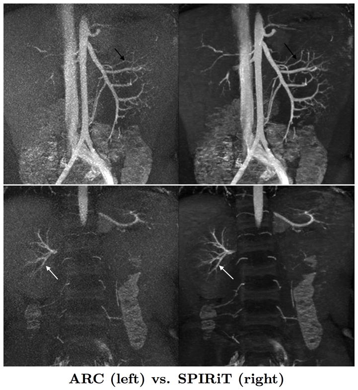
Image quality comparison of GE Product ARC (Autocalibrating Reconstruction for Cartesian imaging) [2] reconstruction (left images) with our ℓ₁-SPIRiT reconstruction (right images). These MRA images of a 5 year old patient were acquired with the 32-channel pediatric torso coil, have FOV 28 cm, matrix size 320 × 320, slice thickness 0.8 mm, and were acquired with 7.2× acceleration, via undersampling 3.6× in the y-direction and 2× in the z-direction. The pulse sequence used a 15 degree flip angle and a TR of 3.9 ms. The ℓ₁-SPIRiT reconstruction shows enhanced detail in the mesenteric vessels in the top images, and and the renal vessels in bottom images.

9 Conclusion

We have presented ℓ₁-SPIRiT, a compressive sensing extension to the SPIRiT parallel imaging reconstruction. Our implementation of ℓ₁-SPIRiT for GPGPUs and multi-core CPUs achieves clinically feasible sub-minute runtimes for highly accelerated, high-resolution scans. We discussed in general terms the software implementation and optimization decisions that contribute to our fast runtimes, and how they apply for the individual operations in ℓ₁-SPIRiT. We presented performance data for both CPU and GPU systems, and discussed how a hybrid parallelization may achieve faster runtimes. Finally, we present an image quality comparison with a competing non-iterative Parallel Imaging reconstruction approach.

In the spirit of reproducible research, our software and scripts to generate the results in this paper are available at: http://www.eecs.berkeley.edu/~mlustig/Software.html

A O(n³) SPIRiT Calibration

As discussed in Section 3, our ℓ₁-SPIRiT calibration solves a least-norm, least-squares (LNLS) fit to the fully-sampled auto-calibration signal (ACS) for each channel’s interpolating coefficients. As each channel’s set of co-efficients interpolates from each of the the n_c channels, the matrix used to solve this system has O(n_c) columns. Solving the n_c least-squares systems independently requires $O(n_c^4)$ time, and is prohibitively expensive. This section derives our algorithm for solving them in $O(n_c^3)$ time using a single matrix-matrix multiplication, single Cholesky factorization, and several inexpensive matrix-vector operations.

We construct a calibration data matrix A from the calibration data in the same manner as GRAPPA [14] and SPIRiT [22] calibration: each row of A is a window of the ACS the same size as the interpolation coefficients. This matrix is Toilets, and multiplication Ax by a vector x ∈ computes the SPIRiT interpolation: $y={\sum }_{i=1}^{n_c}{x}_i\otimes {\text{ACS}}_i$.

The LNLS matrices for each channel differ only by a single column from A. In particular, there is a column of A that is identical to the ACS of each coil. Consider the coil corresponding to column i of A, and let b be that column. We define N = A – be_i′ – A with the i^th column zeroed out. We wish to solve Nx = b in the least-norm least-squares sense, by solving (N^*N +εI)x:= Ñx = N^*b. The runtime of our efficient algorithm is dominated computing the product N^*N and computing the Cholesky factorization LL^* = Ñ.

Our derivation begins by noting that:

$$\begin{array}{l}\stackrel{\sim }{N}=N^{\ast }N+\epsilon I\\ ={(A-{be}^{\prime })}^{\ast }(A-{be}^{\prime })+\epsilon I\\ =A^{\ast }A+\epsilon I-\stackrel{\sim }{b}{e}^{\prime }-e{\stackrel{\sim }{b}}^{\ast }\end{array}$$

Where we have defined b̃ = A^*b with entry i multiplied by $\frac{1}{2}$ to avoid adding eb^*be′. If we have a Cholesky factorization LL^* = A^*A + εI:

$$\begin{array}{l}\stackrel{\sim }{N}={LL}^{\ast }-\stackrel{\sim }{b}{e}^{\prime }-e{\stackrel{\sim }{b}}^{\ast }\\ ={LL}^{-1}({LL}^{\ast }-\stackrel{\sim }{b}{e}^{\prime }-e{\stackrel{\sim }{b}}^{\ast })L^{-\ast }{L}^{\ast }\\ =L(I-\widehat{b}{\widehat{e}}^{\ast }-\widehat{e}{\widehat{b}}^{\ast })L^{\ast }\end{array}$$

Where we’ve defined b̂ = L⁻¹ b̃ = L⁻¹ A^*b, and ê = L⁻¹e. These vectors can be computed with BLAS2 triangular solves and matrix-vector multiplications. In fact, we can aggregate the b’s and e’s from all parallel imaging channels into matrices and compute all b̂’s and ê’s with highly efficient BLAS3 solves. Now, to solve the system of equations Ñx = b̃:

$$\begin{array}{l}x={\stackrel{\sim }{N}}^{-1}\stackrel{\sim }{b}\\ ={(L(I-\widehat{b}{\widehat{e}}^{\ast }-\widehat{e}{\widehat{b}}^{\ast })L^{\ast })}^{-1}\stackrel{\sim }{b}\\ =L^{-\ast }{(I-\widehat{b}{\widehat{e}}^{\ast }-\widehat{e}{\widehat{b}}^{\ast })}^{-1}{L}^{-1}\stackrel{\sim }{b}\end{array}$$

It remains to compute the inverse of (I − b̂ê^* − êb̂^*). We can define two matrices B̂, Ê ∈ , where B̂ = − (b̂, ê), and Ê = (ê, b̂). Using the Sherman-Morrison-Woodbury identity:

$$\begin{array}{l}{(I-\widehat{b}{\widehat{e}}^{\ast }-\widehat{e}{\widehat{b}}^{\ast })}^{-1}={(I+\widehat{B}{\widehat{E}}^{\ast })}^{-1}\\ =I-\widehat{B}{(I+{\widehat{E}}^{\ast }\widehat{B})}^{-1}{\widehat{E}}^{\ast }\end{array}$$

Note that I + Ê^*B̂ is a 2 × 2 matrix that is very inexpensive to invert. Thus we have our final algorithm:

$$\begin{array}{l}L\leftarrow \text{chol}(A^{\ast }A+\epsilon I)\\ \widehat{b}\leftarrow L^{-1}{A}^{\ast }b\\ \widehat{e}\leftarrow L^{-1}e\\ \widehat{B}\leftarrow -\left(\widehat{b},\widehat{e}\right)\\ \widehat{E}\leftarrow \left(\widehat{e},\widehat{b}\right)\\ x\leftarrow L^{-\ast }(I-\widehat{B}{(I+{\widehat{E}}^{\ast }\widehat{B})}^{-1}{\widehat{E}}^{\ast })\widehat{b}\end{array}$$

References

- 1.Akcakaya Mehmet, Basha Tamer, Manning Warren, Nam Seunghoon, Nezafat Reza, Stehning Christian, Tarokh Vahid. A gpu implementation of compressed sensing reconstruction of 3d radial (kooshball) acquisition for high-resolution cardiac mri. Proceedings of the International Society for Magnetic Resonance in Medicine; 2011. [Google Scholar]
- 2.Beatty PJ, Brau A, Chang S, Joshi S, Michelich C, Bayram E, Nelson T, Herfkens R, Brittain J. A method for autocalibrating 2d-accelerated volumetric parallel imaging with clinically practical reconstruction times. Proceedincs of the Joint Annual Meeting ISMRM-ESMRMB; 2007. p. 1749. [Google Scholar]
- 3.Beatty PJ, Nishimura DG, Pauly JM. Rapid gridding reconstruction with a minimal oversampling ratio. IEEE Trans Med Imaging. 2005 Jun;24:799–808. doi: 10.1109/TMI.2005.848376. [DOI] [PubMed] [Google Scholar]
- 4.Block Kai Tobias, Uecker Martin, Frahm Jens. Undersampled radial mri with multiple coils. iterative image reconstruction using a total variation constraint. Magn Reson Med. 2007 Jun;57(6):1086–98. doi: 10.1002/mrm.21236. [DOI] [PubMed] [Google Scholar]
- 5.Buccigrossi RW, Simoncelli EP. Image compression via joint statistical characterization in the wavelet domain. IEEE Trans Image Processing. 1999;8:1688–1701. doi: 10.1109/83.806616. [DOI] [PubMed] [Google Scholar]
- 6.Buehrer Martin, Pruessmann Klaas P, Boesiger Peter, Kozerke Sebastian. Array compression for MRI with large coil arrays. Magn Reson Med. 2007;57(6):1131–9. doi: 10.1002/mrm.21237. [DOI] [PubMed] [Google Scholar]
- 7.Candès EJ, Romberg J, Tao T. Robust uncertainty principles: Exact signal reconstruction from highly incomplete frequency information. IEEE Transactions on Information Theory. 2006;52:489–509. [Google Scholar]
- 8.Chang Ching-Hua, Ji Jim. Compressed sensing mri with multichannel data using multicore processors. Magn Reson Med. 2010 Oct;64(4):1135–9. doi: 10.1002/mrm.22481. [DOI] [PubMed] [Google Scholar]
- 9.Daubechies I, Defrise M, De Mol C. An iterative thresholding algorithm for linear inverse problems with a sparsity constraint. Comm Pure Applied Mathematics. 2004;57:1413–1457. [Google Scholar]
- 10.Donoho DL. Compressed sensing. IEEE Transactions on Information Theory. 2006;52:1289–1306. [Google Scholar]
- 11.Donoho DL, Johnstone IM. Ideal spatial adaptation via wavelet shrinkage. Biometrika. 1994;81:425–455. [Google Scholar]
- 12.Asanovic, et al. Technical report. EECS Department, University o California; berkeley: Dec, 2006. The landscape of parallel computing research: a view from berkeley. [Google Scholar]
- 13.Gregerson Anthony. Technical report. University of Wisconsin; Madison: 2008. Implementing fast mri gridding on gpus via cuda. [Google Scholar]
- 14.Griswold Mark A, Jakob Peter M, Heidemann Robin M, Nittka Mathias, Jellus Vladimir, Wang Jianmin, Kiefer Berthold, Haase Axel. Generalized autocalibrating partially parallel acquisitions (GRAPPA) Magn Reson Med. 2002;47(6):1202–10. doi: 10.1002/mrm.10171. [DOI] [PubMed] [Google Scholar]
- 15.Huang Feng, Chen Yunmei, Yin Wotao, Lin Wei, Ye Xiaojing, Guo Weihong, Reykowski Arne. A rapid and robust numerical algorithm for sensitivity encoding with sparsity constraints: self-feeding sparse sense. Magn Reson Med. 2010 Oct;64(4):1078–88. doi: 10.1002/mrm.22504. [DOI] [PubMed] [Google Scholar]
- 16.Kim Daehyun, Trzasko Joshua D, Smelyanskiy Mikhail, Haider Clifton R, Manduca Armando, Dubey Pradeep. High-performance 3d compressive sensing mri reconstruction. Conf Proc IEEE Eng Med Biol Soc. 2010;2010:3321–4. doi: 10.1109/IEMBS.2010.5627493. [DOI] [PubMed] [Google Scholar]
- 17.Knoll Florian, Clason Christian, Bredies Kristian, Uecker Martin, Stollberger Rudolf. Parallel imaging with nonlinear reconstruction using variational penalties. Magn Reson Med. 2011 Jun; doi: 10.1002/mrm.22964. [DOI] [PMC free article] [PubMed] [Google Scholar]
- 18.Lai Peng, Lustig Michael, Brau Anja CS, Vasanawa la Shreyas, Beatty Philip J, Alley Marcus. Efficient ℓ1-SPIRiT reconstruction (ESPIRiT) for highly accelerated 3D volumetric MRI with parallel imaging and compressed sensing. Proceedings of the International Society for Magnetic Resonance in Medicine; 2010. p. 345. [Google Scholar]
- 19.Liang Dong, Liu Bo, Wang Jiunjie, Ying Leslie. Accelerating sense using compressed sensing. Magn Reson Med. 2009 Dec;62(6):1574–84. doi: 10.1002/mrm.22161. [DOI] [PubMed] [Google Scholar]
- 20.Lustig M, Alley M, Vasanawala S, Donoho DL, Pauly JM. ℓ1-SPIRiT: Autocalibrating parallel imaging compressed sensing. Proceedings of the International Society for Magnetic Resonance in Medicine; 2009. p. 379. [Google Scholar]
- 21.Lustig Michael, Donoho David L, Pauly John Mark. Sparse MRI: The application of compressed sensing for rapid MR imaging. Magn Reson Med. 2007;58(6):1182–1195. doi: 10.1002/mrm.21391. [DOI] [PubMed] [Google Scholar]
- 22.Lustig Michael, Pauly John M. SPIRiT: Iterative self-consistent parallel imaging reconstruction from arbitrary k-space. Magnetic Resonance in Medicine. 2010;64(2):457–471. doi: 10.1002/mrm.22428. [DOI] [PMC free article] [PubMed] [Google Scholar]
- 23.Mattson Timothy, Sanders Beverly, Massingill Berna. Patterns for parallel programming. 1. Addison-Wesley Professional; 2004. [Google Scholar]
- 24.Murphy M, Keutzer K, Vasanawala S, Lustig M. Clinically feasible reconstruction time for ℓ1-SPIRiT parallel imaging and compressed sensing MRI. Proceedings of the International Society for Magnetic Resonance in Medicine; 2010. p. 4854. [Google Scholar]
- 25.Nvidia. [Online; accessed 25 July, 2011];Compute Unified Device Architecture (Cuda) http://www.nvidia.com/object/cuda_get.html.
- 26.Obeid Nady, Atkinson Ian, Thulborn Keith, Hwu Wen-Mei. Gpu-accelerated gridding for rapid reconstruction of non-cartesian mri. Proceedings of the International Society for Magnetic Resonance in Medicine; 2011. [Google Scholar]
- 27.Otazo Ricardo, Kim Daniel, Axel Leon, Sodickson Daniel K. Combination of compressed sensing and parallel imaging for highly accelerated first-pass cardiac perfusion mri. Magn Reson Med. 2010 Sep;64(3):767–76. doi: 10.1002/mrm.22463. [DOI] [PMC free article] [PubMed] [Google Scholar]
- 28.Pruessmann KP, Weiger M, Börnert P, Boesiger P. Advances in sensitivity encoding with arbitrary k-space trajectories. Magn Reson Med. 2001 Oct;46(4):638–51. doi: 10.1002/mrm.1241. [DOI] [PubMed] [Google Scholar]
- 29.Pruessmann KP, Weiger M, Scheidegger MB, Boesiger P. Sense: sensitivity encoding for fast mri. Magn Reson Med. 1999 Nov;42(5):952–62. [PubMed] [Google Scholar]
- 30.Roujol S, de Senneville BD, Vahala E, Sorensen TS, Moonen C, Ries M. Online real-time reconstruction of adaptive tsense with commodity cpu/gpu hardware. Magnetic Resonance in Medicine. 2009;62:1658–1664. doi: 10.1002/mrm.22112. [DOI] [PubMed] [Google Scholar]
- 31.Sodickson DK, Manning WJ. Simultaneous acquisition of spatial harmonics (smash): fast imaging with radiofrequency coil arrays. Magn Reson Med. 1997 Oct;38(4):591–603. doi: 10.1002/mrm.1910380414. [DOI] [PubMed] [Google Scholar]
- 32.Sorensen Thomas Sangild, Prieto Claudia, Atkinson David, Hansen Michael Schacht, Schaeffter Tobias. Gpu accelerated iterative sense reconstruction of radial phase encoded whole-hyeart mri. Proceedings of the International Society for Magnetic Resonance in Medicine; 2010. [Google Scholar]
- 33.Stone Samuel S, Haldar Justin P, Tsao Stephanie C, Hwu Wenmei W, Liang Zhi-Pei, Sutton Bradley P. Accelerating advanced mri reconstructions on gpus. Proceedings of the 5th conference on Computing Frontiers; 2008. [DOI] [PMC free article] [PubMed] [Google Scholar]
- 34.Trzasko Joshua D, Haider Clifton R, Borisch Eric A, Campeau Norbert G, Glockner James F, Riederer Stephen J, Manduca Armando. Sparsecapr: Highly accelerated 4d cemra with parallel imaging and nonconvex compressive sensing. Magn Reson Med. 2011 Oct;66(4):1019–32. doi: 10.1002/mrm.22892. [DOI] [PMC free article] [PubMed] [Google Scholar]
- 35.Uecker Martin, Hohage Thorsten, Block Kai Tobias, Frahm Jens. Image reconstruction by regularized nonlinear inversion–joint estimation of coil sensitivities and image content. Magn Reson Med. 2008 Sep;60(3):674–82. doi: 10.1002/mrm.21691. [DOI] [PubMed] [Google Scholar]
- 36.Uecker Martin, Zhang Shuo, Frahm Jens. Nonlinear inverse reconstruction for real-time mri of the human heart using undersampled radial flash. Proceedings of the International Society for Magnetic Resonance in Medicine; 2010. [DOI] [PubMed] [Google Scholar]
- 37.Vasanawala Shreyas S, Alley Marcus T, Hargreaves Brian A, Barth Richard A, Pauly John M, Lustig Michael. Improved pediatric MR imaging with compressed sensing. Radiology. 2010 Aug;256(2):607–16. doi: 10.1148/radiol.10091218. [DOI] [PMC free article] [PubMed] [Google Scholar]
- 38.Vasanawala SS, Murphy MJ, Alley MT, Lai P, Keutzer K, Pauly JM, Lustig M. Practical parallel imaging compressed sensing MRI: Summary of two years of experience in accelerating body MRI of pediatric patients. Proceedings of IEEE International Symposium on Biomedical Imaging; Chicago. 2011. pp. 1039–1043. [DOI] [PMC free article] [PubMed] [Google Scholar]
- 39.Wu Bing, Millane Rick P, Watts Richard, Bones Philip J. Prior estimate-based compressed sensing in parallel mri. Magn Reson Med. 2011 Jan;65(1):83–95. doi: 10.1002/mrm.22545. [DOI] [PubMed] [Google Scholar]
- 40.Wu Xiao-Long, Gai Jiading, Lam Fan, Fu Maojing, Haldar Justin, Zhuo Yue, Liang Zhi-Pei, Hwu Wen mei, Sutton Bradley. Impatient mri: Illinois massively parallel acceleration toolkit for image reconstruction with enhanced throughput in mri. Proceedings of the IEEE International Symposium on Biomedical Imaging (ISBI); 2011. [Google Scholar]
- 41.Ying Leslie, Sheng Jinhua. Joint image reconstruction and sensitivity estimation in sense (jsense) Magn Reson Med. 2007 Jun;57(6):1196–202. doi: 10.1002/mrm.21245. [DOI] [PubMed] [Google Scholar]
- 42.Zhang Tao, Lustig Michael, Vasanawala Shreyas, Pauly John. Array compression for 3d cartesian sampling. Proceedings of the International Society for Magnetic Resonance in Medicine; 2011. p. 2857. [Google Scholar]
- 43.Zhuo Yue, Wu Xiao-Long, Haldar Justin P, Hwu Wen-Mei W, Liang Zhi-Pei, Sutton Bradley P. Multi-gpu implementation for iterative mr image reconstruction with field correction. Proceedings of the International Society for Magnetic Resonance in Medicine; 2010. [Google Scholar]