Parallel β-sheet vibrational couplings revealed by 2D IR spectroscopy of an isotopically labeled macrocycle: Quantitative benchmark for the interpretation of amyloid and protein infrared spectra

Abstract

Infrared spectroscopy is playing an important role in the elucidation of amyloid fiber formation, but the coupling models that link spectra to structure are not well tested for parallel β-sheets. Using a synthetic macrocycle that enforces a two stranded parallel β-sheet conformation, we measured the lifetimes and frequency for six combinations of doubly ¹³C=¹⁸O labeled amide I modes using 2D IR spectroscopy. The average vibrational lifetime of the isotope labeled residues was 550 fs. The frequen cies of the labels ranged from 1585 to 1595 cm⁻¹, with the largest frequency shift occurring for in-register amino acids. The 2D IR spectra of the coupled isotope labels were calculated from molecular dynamics simulations of a series of macrocycle structures generated from replica exchange dynamics to fully sample the conformational distribution. The models used to simulate the spectra include through-space coupling, through-bond coupling, and local frequency shifts caused by environment electrostatics and hydrogen bonding. The calculated spectra predict the linewidths and frequencies nearly quantitatively. Historically, the characteristic features of β-sheet infrared spectra have been attributed to through-space couplings such as transition dipole coupling. We find that frequency shifts of the local carbonyl groups due to nearest neighbor couplings and environmental factors are more important, while the through space couplings dictate the spectral intensities. As a result, the characteristic absorption spectra empirically used for decades to assign parallel β-sheet secondary structure arises because of a redistribution of oscillator strength, but the through-space couplings do not themselves dramatically alter the frequency distribution of eigenstates much more than already exists in random coil structures. Moreover, solvent exposed residues have amide I bands with >20 cm⁻¹ linewidth. Narrower linewidths indicate that the amide I backbone is solvent protected inside the macrocycle. This work provides calculated and experimentally verified couplings for parallel β-sheets that can be used in structure-based models to simulate and interpret the infrared spectra of β-sheet containing proteins and protein assemblies, such as amyloid fibers.

INTRODUCTION

Vibrational spectroscopy is one of the most commonly used techniques for assessing the secondary structure content of proteins.¹ It is often the first tool that a researcher uses to assess structure in membrane bound proteins and to monitor dynamics in protein folding, to name only two applications. More than 50 years ago it was recognized that the relationship between protein secondary structure and the observed amide I absorption band is caused by vibrational coupling between the amide groups of the protein backbone.^2,3 That realization enabled researchers to begin modeling the infrared spectra of proteins using a local mode or excitonic-type Hamiltonian in which only the amide I vibrational modes need to be considered.^4,5 Excitonic models have become a key tool in the interpretation of the infrared spectra of proteins, because they enable a very straightforward and intuitive structure-spectra relationship in contrast to the vibrational modes of most other molecules, and even the other protein amide modes for which few simple models currently exist.^6-9

In the last few years, improvements to the methods for calculating the parameters of these excitonic Hamiltonians is enabling a transition from semi-quantitative to quantitative simulations of protein amide I spectra. The two primary ingredients for exciton Hamiltonians are the frequencies for each of the individual amide groups and the coupling between pairs. Amide I frequencies are now being calculated from mixed quantum/classical theories using parameters developed from ab initio or empirical fitting parameters.^9-15 These methods not only account for hydrogen bonding, but also frequency shifts caused by microsolvation, local dielectric effects, and the dependence of the vibrational mode itself on the dihedral angles. Ab initio, transition charge, and transition dipole density calculations are some ways of obtaining the couplings.^{5,13,14,16-22} With an exciton Hamiltonian in place, mixed quantum/classical lineshape theory is used to simulate the infrared spectra.^15,23,24 The result is an infrared spectrum that includes the molecular structure, its surrounding environment, and the structural dynamics of both. Thus, with a quantitative theory in hand, structural and dynamical information can be interpreted from infrared spectroscopy and 2D IR spectroscopy in particular.

While exciton models are improving and simulations of proteins are abundant in the literature, the accuracy with which infrared spectra can be calculated is not fully tested. Pieces of the modeling have been developed quite accurately. For example, the frequency shifts caused by electrostatics and hydrogen bonding of the environment have been developed using empirical fits to model system.^15,25 The frequency shift caused by couplings and dihedral angles is less well tested. Part of the problem is of an experimental nature. The infrared spectra of proteins and even small peptides are too congested to resolve individual amide I absorption bands. As a result, when a simulation does not match an experiment, it is difficult to ascertain which part of the exciton model failed. One way to relieve congestion is through the use of isotope labeling. ¹³C¹⁸O-labeling of backbone carbonyl groups enables individual or subsets of amide I modes to be spectroscopically resolved and vibrationally decoupled from the unlabeled residues.^26-29 As a result, one can measure the frequencies of individual residues or pairs of amide I modes. These measurements provide the fundamental quantities necessary to test and calibrate well-defined elements in the excitonic Hamiltonian.

It is especially important to benchmark the accuracy for common secondary structures and in typical environments. Using various combinations of isotope labeling and either 1D or 2D IR spectroscopy, the fundamental coupling constants and environmental frequency shifts for many of the most common protein secondary structures have been determined in a variety of environments. Soluble helices have been isotopically labeled at single, double and quadruple positions to probe the most important coupling constants in an α-helix.^27,30,31 Isotope labeling has been used to study the coupling in 30-10 helices.³² Frequency shifts associated with environments have been characterized in soluble and membrane bound α-helices, including surface bound monomers and α-helical bundles with and without water pores.^33-37 Many of the coupling constants for β-turns and anti parallel β-sheets have been measured with isotope labeling and 2D IR spectroscopy.^38-40 As a result of these experiments, there is reasonable certainty in the accuracy to which α-helices, turns and anti-parallel β-sheets are modeled. Thus, for these secondary structures and environments, there exist benchmark calculations and experiments that quantify the accuracy of the structure/spectra relationship.

Bench-marking parallel β-sheets has proven to be more difficult than for any other common secondary structure, because small peptides do not readily adopt parallel β-sheet structure.^41,42 Among proteins, parallel β-sheets are less common than antiparallel β-sheets. Parallel β-sheets often occur in large proteins repetitive structural motifs such as β-solenoids, leucine rich repeats, and TIM barrels; this secondary structure is often found in amyloid aggregates as well.^43-45 Parallel strands can occur in mixed parallel/antiparallel β-sheets, with the strand orientations enforced by the overall protein fold.⁴⁶ None of these natural systems is amenable to the systematic studies required for establishing the IR signatures we seek. Proteins that are large enough to form parallel β-sheets are necessarily difficult to label isotopically at specific sites. In aggregates, such as amyloid fibers, one cannot fully control the arrangement of isotope labels, as would be necessary to probe all key coupling constants. As a result of these technical problems, the coupling constants of parallel β-sheet are probably the least well characterized of all the common secondary structure elements, even as attention to parallel β-sheet is growing with the rising interest in protein aggregation diseases and biocompatible peptide gels.^47,48 Current coupling models have not been fully tested, but they are nevertheless used in numerous experimental and theoretical analyses of β–sheet proteins and amyloids.⁴⁹

In this paper, we focus on experimentally testing theoretical models for the coupling between variously juxtaposed residue pairs within parallel β-sheets, and environmental effects on this coupling. To overcome the problems associated with natu ral parallel β-sheets, we utilize the synthetic peptide macrocycle shown in Fig. 1A. This molecule contains two strand-forming segments, each comprising eight L-α-amino acid residues, that are linked at their N-termini by a glycyl succinyl unit and at their C-termini by D-prolyl-1,2-diamino-1,1-dimethylethyl unit.⁴² These terminal linkers promote parallel β-sheet interactions between the strand segments.⁵⁰ We label pairs of residues isotopically in order to sample interactions between these residues that we believe are the most important matrix elements in the exciton Hamiltonian. The insights gained from these simulations and experiments provide new insight into the interpretation of the infrared spectra of parallel β-sheets within proteins, and our results should inform the design of isotope labeling strategies for testing structural models, such as for amyloid structures.

Figure 1.

Structure of the macrocyclic peptide with numbering scheme for isotope labeled pairs (a). 2D IR data for the unlabeled macrocycle (b) and for the doubly labeled macrocycle (c-h).

MATERIALS AND METHODS

Peptide synthesis and isotope labeling

1-¹³C amino acids (99% ¹³C, Cambridge Isotope) were isotope labeled by acid catalyzed ¹⁸O exchange with ¹⁸O water (95% ¹⁸O, Isotec) under a stream of Argon gas as previously described.²⁹ Isotope labeling efficiency was 84-94% as assessed by LCMS-ESI. Macrocyclic peptides were synthesized using standard microwave assisted Fmoc-based solid phase peptide synthesis techniques with side-chain attachment to the resin to facilitate backbone cyclization as previously described.⁵¹ More details, including purification, characterization, and NOE NMR measurements, are provided in the SI. The dihedral angles in the strand region and the distance between α-carbons of opposite strands fall within the bounds of natural parallel beta-sheets. To prepare the samples for 2D IR experiments, residual TFA from HPLC purification was removed and the peptide simultaneously deuterated by performing three additions of ~1 mL 0.1 DCl in D₂O per mg of peptide with subsequent lyophilization. The peptides were then dissolved in deuterated phosphate buffer (pH 3.8) at about 10 mM concentration.

Spectroscopic Methods

The 2D IR setup used was previously described.²⁹ In brief, 800 nm, 60 fs pulses were generated by a Ti:Sapphire laser, which were converted to six micron light by difference frequency mixing optical parametric amplifier. The mid-IR light was split such that a third of this light was sent through a Ge-AOM to shape the pulse envelope to a double pump pulse. The pump was overlapped spatially and temporally with the remaining mid-IR light (probe) on the sample to generate rephasing and nonrephasing signal heterodyned with the probe beam. The signal and probe were dispersed in the monochromator and detected on one-row array of 64 HCT elements. The pump pulse pair was incrementally varied 0 to 2544 fs in 24 fs steps at the rate of the laser shots (1000 Hz). Lifetime measurements were performed by scanning a translational stage along the pump path.

Molecular Dynamics (MD) Simulations

The initial structure of cyclic peptide was generated according to NMR data. The GROMOS96 53a6 force field^52-54 was used to model the peptide, and the SPC model⁵⁵ was used for water molecules. Parameters for the C-terminal and N-terminal linker were assigned according to the atom types in the force field. The lysine side chains were protonated to give a net charge of +4 for the peptide. Chloride ions were added to neutralize the overall system charge. The system was solvated with 7713 water molecules. All bonds were constrained using the linear constraint solver method.⁵⁶ The system was simulated in the NPT ensemble at 298K and 1 bar using the Nose Hoover thermostat^57,58 and the Parinello-Rahman barostat,⁵⁹ respectively. Long-range electrostatic interactions were treated with a particle-mesh Ewald sum.⁶⁰ Equilibrium MD simulations were performed with an integration time step of 2 fs for 100 ns using the GROMACS molecular simulation package.^61-63

To ensure sufficient sampling of peptide conformations, we performed replica exchange MD (REMD).^64-66 42 replicas were setup at temperatures chosen from 298K to 380K following the procedure of Rathore et al.⁶⁷ Exchanges between neighboring replicas were attempted every 2 ps. 100 ns simulation was performed for each replica, resulting a total simulation time of 4.2 microseconds.

Lineshape and Coupling Calculations

The ¹³C=¹⁸O isotope labels lower the amide I frequency so that the two labeled residues are spectrally isolated from all the other amide modes. Accordingly, they are modeled theoretically as isolated chromophores. For each pair, the amide I Hamiltonian is a 2 × 2 matrix, whose diagonal elements are the local frequencies of the two chromophores and the off-diagonal element is the coupling between them. The local frequencies were calculated using a backbone frequency map,¹⁵ corrected by the nearest-neighbor frequency shift.¹¹ The ¹³C=¹⁸O isotope shift was taken into account by shifting the local frequencies by −66 cm⁻¹, which is concluded from considerations discussed below. Isotopic labeling does not affect the dihedral maps. Couplings between adjacent carbonyls were treated using a nearest-neighbor coupling map.¹¹ Couplings between all other carbon yls groups were calculated. From the Hamiltonian, 2DIR absorptive spectra of the zzzz polarization were calculated,^12,68 using T₁=600 fs and 300 fs for the lifetimes of ν=1 and ν=2, respectively, which matches experimental conditions. The polarization anisotropy effects were accounted as described previously.⁶⁹

To calculate the 2DIR spectra, MD simulations were performed using GROMACS with the same parameters described in the MD Simulations section. To better sample the configurations of the macrocycle, a total of 10 simulations were performed, each starting from configurations 10 ns apart in the 100 ns MD simulations. Each simulation was run for 5 ns and the trajectories were saved every 20 fs for spectra calculations. The spectra and spectral features reported below were averaged over the 10 simulations, and the error bars are presented as twice the standard deviation of the mean. Couplings between the isotope labels and the adjacent uncoupled residues are included through the dihedral maps. To test the effects of other unlabeled residues on our 2×2 Hamiltonian, we diagonalized the full Hamiltonian of both labeled and unlabeled residues for three different configurations. We found that the isotope frequencies were shifted by less than 2 cm⁻¹, confirming that isotope labeling effectively block diagonalizes the Hamiltonian.

RESULTS AND DISCUSSION

Conformation of the macrocyclic peptide in aqueous solution

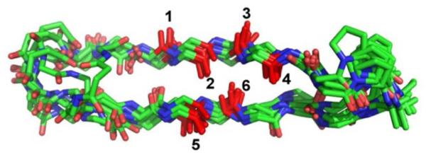
Extensive NMR analysis was conducted to evaluate the conformational behavior of the macrocyclic peptide (see SI for details). Deviations of Cα¹H and ¹³Cα chemical shifts from random coil values, upfield for Cα¹H and downfield for ¹³Cα, are consistent with substantial β-sheet secondary structure over most of the strand segments. Numerous nuclear Overhauser effects (NOEs) were observed between protons on amino acid residues that are far from one another in terms of sequence, but that would be expected to be close to one another spatially upon formation of the expected parallel β-sheet conformation. No NOEs inconsistent with this conformation were detected. A set of 10 low-energy structures derived from NOE-restrained molecular dynamics simulations is shown in Fig. 2. These structures overlap substantially in the parallel β-sheet portion, but deviate a bit at the linker segments. Overall, the NMR data indicate that this macrocyclic peptide provides an excellent scaffold for analysis of IR couplings between amide pairs that have specific spatial juxtapositions within a discrete parallel β-sheet context.

Figure 2.

NMR-NOE structure of the macrocycle overlaid with numbering scheme for isotope labeling indicated.

2D IR spectra of isotopically labeled macrocycles reveal large frequency shifts indicative of structure

Shown in Fig. 1A is the structure of the β-sheet macrocycle used in this study. Seven sets of macrocycles were synthesized. Six macrocycles each had two ¹³C¹⁸O isotope labels, located at residues chosen from 2 of the 6 locations marked in Fig. 1A. One macrocycle was unlabeled. The combinations of isotope labels were selected to probe the inter-strand couplings, intra-strand couplings and the frequency shifts associated with carbonyl groups hydrogen bonded in the β-sheet structure versus those pointed outwards and solvated by water. Shown in Fig. 1B-H are the 2D IR spectra for each of the 7 macrocycles. The unlabeled macrocycle (Fig. 1B) has the strongest absorption at ~1640 cm⁻¹ and stretches to 1680 cm⁻¹, as measured by the diagonal frequency. These features are caused by the β-sheet modes of the unlabeled amino acids. The weaker peak pair at 1612 cm⁻¹ is due to the amide group of the macrocycle linker and the proline backbone amide I mode.⁷⁰ 2D IR spectra of the isotope labeled macrocycles exhibit an additional absorption near 1590 cm⁻¹, which is due to the pairs of ¹³C=¹⁸O labeled residues. It is this absorption band that is the main focus of our study.

We are mainly interested in four sets of quantities. The first set of quantities is the vibrational frequencies of the isotope labeled features, which provide information about the coupling between the isotope labels and their individual amide I frequencies. The second set is the frequencies of the unlabeled amide feature, because these frequencies provide information about the extent that the vibrational excitons are delocalization across the parallel β-sheet. The third set is the 2D lineshapes of the isotope labels, which are a measure of the homogeneous and inhomogeneous vibrational dynamics, and thus provides information on the distribution of frequencies caused by the protein and solvent structural distribution. Finally, we measure the vibrational lifetimes of the isotope labels, to ascertain the proportion of the lineshape governed by vibrational relaxation and to correlate hydration to lifetime, as has been observed in other systems.⁷¹

It is immediately apparent from the data that the isotope labels are sensitive to the macrocycle structure and environment. Plotted in Fig. 3A are slices through the diagonals (ω_probe=ω_pump) of the 2D IR spectra. Simple inspection reveals that the isotope label frequency spans 10 cm⁻¹ and has a linewidth that ranges from very sharp to quite broad. The peak maximum of the unlabeled features near 1640 cm⁻¹ also depends on the location of the isotope labels, indicating that the delocalization of the excitons across the β-sheets is disrupted by the labels. To quantitatively extract the frequencies and linewidths of these features, we fit these slices to three Gaussians: one for the label, one for the proline absorption, and one for the unlabeled residues. The frequency of the proline Gaussian was constrained to +/− 2 cm⁻¹ at 1610 cm⁻¹, since its frequency should not vary from sample to sample. Because of the large frequency separation, the fit to the unlabeled amide absorption band has little influence on the isotope labeled band. A single Gaussian was used to fit the isotope labeled region because the individual isotope labels are not resolved. We did not expect to resolve the individual residues, because previous studies have found that the typical frequency dependence of an isotope labeled amide I band is about 10 cm⁻¹.^26-28,37 Nonetheless, the peak maximum and linewidth, which will correspond to the summation of the two labels, is sensitive to structure as our data shows and has also been true in isotope labeled α-helices.³⁰ The fits are shown in the Supplemental Fig. S20. The extracted frequencies and lineshapes are plotted in Fig. 3B-C (red). These fits provide three of the desired experimental quantities named above.

Figure 3.

Overlapped slices along the diagonal of experimental 2DIR spectra (a), peak frequencies (b), and linewidths (c). Slices are normalized to their maximum intensity.

From this data, we note a few observations. First, regarding the isotope labeled region of the spectra, the sample with the lowest frequency absorption is the (3,6) labeled peptide. These labels lie on different strands and are in-register. In the literature, it is commonly thought that the coupling between these two residues is the most important, because transition dipole coupling (which is one of the oldest and most often used coupling models) predicts this coupling to be the largest in parallel β-sheets.^21,72,73 The frequency of the (3,6) labeled pair is consistent with this historical conclusion. Second, the ¹²C¹⁶O feature exhibits the largest blue shift for all three peptides in which the two labels are located on the same strand. Macrocycles in which the labels are located on opposite strands shift only half as much. This observation reveals that, while inter-strand couplings may be the largest in β-sheets, intra-strand couplings are equally as important for interpreting infrared spectra. If only inter-strand couplings were important, then a parallel β-sheet spectrum could be modeled using a linear chain of coupled oscillators and so it would not make a difference if the two labels were on the same or opposite strands, because the same number of linear chains would be disrupted (barring the (3,6) label). The observation that isotope labeling one strand twice breaks up the β-sheet excitons more than labeling each strand once, signifies that the vibrational modes of the β-sheets are delocalized about equally along and across the strands. Third, the spectrum of the (3,5) labeled peptide, in which both labels face outward, has a much broader linewidth than any of the others samples. This observation is consistent with environmental disorder being more important for residues on the outside than those that point inward and are less solvent exposed. As we discuss below, these empirical observations are confirmed by our simulations.

Structural distribution of the macrocycle

Infrared spectroscopy samples molecular conformations on the timescale of a few picoseconds. Thus, it provides a snapshot of the structural distribution on a timescale in which only the fast solvent rearrangements or hydrogen bonding fluctuations occur. As a result, the infrared spectrum can be calculated from a molecular dynamics simulation of only 1 or 2 nanoseconds,^9,14,15,21 which is an exciting feature of infrared spectroscopy because nanosecond simulations are easily accessible with modern computers. However, since infrared spectroscopy is an ensemble measurement, it measures all structural conformations present in the sample. Thus, to properly simulate an FTIR or 2D IR spectrum, one needs to sample and obtain the relative weightings for the conformational distribution.

The structure of the parallel macrocycle is well character ized by NMR. We took two approaches to characterize the distribution of structures. First, we ran a 100 ns trajectory. Second, we employed replica exchange dynamics. In both cases, the distribution of structures is similar to the distribution generated from using the experimental NMR constraints. As a result, we are confident that we have fully sampled the peptide structural distribution.

Shown in Fig. 2 is an overlay of 10 NMR derived structures. Notice that the macrocycle becomes structurally disordered at the two ends, but is much more stable in the middle where the isotope labels reside. In the middle, all 10 structures retain their inter-strand hydrogen bonding. Deviations from the average structure come mostly from out of plane rotations. At no point in any of the simulations is a large-scale disruption or puckering of the macrocycle observed. Thus, frequency fluctuations in the 2D IR spectra will come from the out-of-plane rotations, which will alter the coupling constants, hydrogen bond shifts associated with these rotations, and the effects of solvation (which are not shown in this Figure).

Modeling parameters and simulated infrared spectra

Using the distribution of macrocycle structures discussed above, we have simulated the 2D IR spectra of the isotope labels. We aim to obtain insights into three different sets of parameters that contribute to these simulations. These parameters are the local mode frequency shifts caused by environmental electrostatics and hydrogen bonding, the dependence of the local mode frequency on the dihedral angles, and the model used to calculate through-space coupling. We briefly review these parameters below.

The excitonic Hamiltonian is a matrix whose diagonal elements represent the local mode frequencies of the individual amide I vibrational modes and off-diagonal elements contain the couplings between these vibrational modes.⁷⁴ There are two factors that contribute to the local mode frequency. The first is the dependence of the local mode frequency on its environment. In general, electrostatic forces from the environment red shift the vibrational frequency from the gas-phase value, with larger shifts occurring for more polar environments. However, the precise frequency shift is set by the instantaneous structure of the microenvironment.^15,23,75 Moreover, hydrogen bonding also contributes, which generally causes an additional red shift. To simulate these two factors, several methods have been developed.^15,23,76 We utilize a correlation that has been established between the C and N atoms of the amide I mode with the electrostatic field of the environment (including the protein, except for the nearest amide atoms (C, O, N, H) and the two nearest α-carbons). The correlation is given by:

$${\omega }_i=1684+7729E_{\mathit{ci}}-3576E_{\mathit{Ni}},$$ Eq.(1)

where E_Ci and E_Ni are the projections of the electrostatic field onto the C and N atoms in the C=O bond direction. ω_i is in units of cm⁻¹ and the fields are in atomic units. This correlation has been obtained by empirically fitting the infrared spectra for the model compound, N-methylacetamide, in a variety of solvents.¹⁵ This model has been shown to reproduce the IR spectra of model peptides with various secondary structures,⁷⁷ including the rat and human amylin peptides, and the isotope-labeled 2DIR spectra of human amylin fibril well.⁴⁹

The second factor that contributes to the diagonal frequencies is the character of the local mode as a function of the dihedral angles.^78,79 For a particular amide group, the effect of the adjacent amide groups on its local frequency is quantum mechanical in nature and cannot be described by simple electrostatics. We have utilized the nearest neighbor frequency shift maps developed from gas phase ab initio calculations to account for such effects.¹⁸ Shown in Fig. 4 are the frequency shifts for these effects determined from gas phase ab initio calculations. Fig. 4A is the map for the frequency shift as a function of the dihedral angles to the N-terminal side of the amide I mode being calculated and Fig. 4B is the map for the C-terminal side. The two values are added, which in turn are added to the environmental frequency shift calculated from Eq. 1. The total sum is the final value used for the diagonal element in the exciton Hamiltonian for that particular amide I mode.

Figure 4.

Frequency shift dependency on dihedral angle about the N atom (a) and C atom (b) in the peptide bond. The conformation of a parallel β–sheet is highlighted in red and the conformation of an α–helix in blue.

The third set of parameters in modeling the Hamiltonian are the off-diagonal elements for the couplings. Models for the vibrational couplings have been studied for decades. These include transition dipole coupling, transition charge coupling, and transition dipole density coupling models.^5,11,16-19 In general, these three coupling models represent three different levels of approximation to the coupling caused by electrostatics. Transition dipole coupling was the first coupling model proposed to explain the dependence of infrared spectra on peptide conformation.⁵ At close distances, it is not accurate,^18,19 and in some cases electrostatics may break down, such as for nearest neighbors. In these situations, one can use ab initio calculations to compute the coupling constants.¹⁸ For our simulations, presented below, we have used an ab initio derived map for nearest neighbor couplings.^11,80

The final piece of necessary information is the inherent frequency shift caused by the ¹³C=¹⁸O isotope label itself. Surprisingly, this quantity is not well established. A back-of-the-envelope calculation based on changes to the reduced mass and assuming that the amide I mode solely consists of C and O motions, puts the frequency shift at −77 cm⁻¹. Electronic structure calculations on N-methylacetamide predict −71 cm⁻¹,⁸¹ and our own calculations on N-methylacetamide give −43 cm⁻¹ for ¹³C labeling alone (Lu Wang, unpublished).¹⁵ In their development of empirical frequency maps, Wang et al. used approximately these frequency shifts, which provided reasonable agreement with several different experiments.^49,82 Experimental values of the ¹³C¹⁸O shift reported in the literature range from −75 to −59.6 cm⁻¹.^{15,26,30,81,83,84} This range of values is probably due to two factors: (1) the use of model compounds that do not accurately represent an amide I mode in a peptide and (2) the frequency shift is mistakenly referenced to an absorption band that is itself shifted due to excitonic coupling. While the ¹³C¹⁸O frequency shift is not well established, the frequency shift caused by ¹³C coupling is consistently reported in the literature at 40 cm⁻¹,^38,75,85 and has been especially well benchmarked by recent uniform ¹³C protein expression studies.⁸⁶ Assuming this experimental value for ¹³C is correct, then the ab initio calculations over predict the frequency shift. Therefore, to obtain the ¹³C¹⁸O shift, we take the experimental ¹³C frequency shift and scale it by the ratio of the ab initio frequencies, which yields 40*71/43 = 66 cm⁻¹. Thus, we calculate the frequency shift from the best available data and a reliable calculation.^36,87

Shown in Fig. 5 are the diagonal slices through the computed 2D IR spectra for each of the isotope label pairs. These spectra are calculated using the molecular dynamics simulations and the three parameters discussed above along with mixed quantum/classical lineshape theory. Details of the simulation methods are given in the Supplemental and elsewhere.¹⁵ For each pair of labels, spectra are shown for each individual isotope label, the sum of the individual isotope labels (by zeroing the off-diagonal matrix elements), and the spectrum resulted from full coupling. In these spectra, couplings other than nearest neighbor were calculated using transition dipole coupling. The corresponding coupling strengths are given in Table 2 and in the figure.

Figure 5.

Calculated 2DIR diagonal spectra for each isotope label without coupling (red and blue), the sum of the pair’s intensity without coupling (cyan), and the sum with coupling (black).

Table 2.

Coupling calculated for each isotope label pair using TDC and TCC coupling models.

Isotope Label	TDC Krimm	TDC Torii 98	TCC Hamm	TCC Jansen
2,4	2.18 ± 0.49	1.16 ± 0.24	1.52 ± 0.38	1.08 ± 0.55
1,4	-0.36 ± 0.15	-0.22 ± 0.09	-0.36 ± 0.13	-0.10 ± 0.15
3,6	-10.80 ± 1.38	-6.14 ± 0.73	-8.82 ± 1.12	-7.03 ± 0.82
4,6	-0.55 ± 3.68	1.63 ± 1.58	1.96 ± 1.59	1.10 ± 2.03
3,5	2.00 ± 0.24	1.33 ± 0.22	2.05 ± 0.45	1.56 ± 0.33

From these simulations, one ascertains the following. First, amide I modes whose carbonyl group point away from the sheets have lower frequencies and broader linewidths. The lower frequencies are a result of the electrostatic fields of the water being larger than the peptide backbone. The larger bandwidth is because the water is more disordered than the backbone. Second, the summation of the individual spectra closely resembles the coupled mode spectra, except for the (3,6) pair. The similarity is a consequence of the small couplings strengths (<2 cm⁻¹) and the large differences in local mode frequencies for most pairs. Third, none of the pairs have a large enough coupling strength to significantly alter the frequency distribution. Not even the (3,6) pair spans a frequency range larger than the individual oscillators. Fourth, the major effect of the coupling is to redistribute the oscillator strength. The most obvious redistribution is for the (3,6) pair, which causes the spectrum to maximize at the lowest frequency even though the lower frequency oscillator has a much weaker intensity than its high frequency counterpart. All six pairs studied here exhibit a redistribution of oscillator strength either to lower or higher frequencies, due to the sign of the coupling constant and the relative angles of the labeled carbonyls.⁷⁴ These observations provide a basis for us to intuitively understand the infrared spectra of β-sheets.

Comparison to experiment

With experimental and simulated results in hand, we compare the two to test the accuracy of the structural/spectra relationship. Shown in Fig. 6 are the experimental values of the maximum frequency and linewidth for the isotope labeled region as extracted from the fits to the spectra described above. In a similar manner, we have plotted the peak frequency and linewidth taken from the simulations. The simulated spectra have been calculated using two different transition dipole coupling (TDC) models and two transition charge coupling (TCC) models.^11,16,18,19 TDC is by far the simplest model that describes the interactions between non-adjacent amide groups.⁵ It assumes that couplings between these chromophores are electrostatic in nature and can be represented by the interaction of the transition dipoles. The two TDC models differ in the location, orientation and magnitude of the transition dipole relative to the C, O and N atoms that comprise the amide I mode.^16,18 The model listed as TDC Krimm, refers to the parameters first proposed by Krimm and coworkers.^88,89 The TDC Torii98 model was developed by Torii in 1998 through ab initio molecular orbital (MO) calculations.¹⁸ TCC models have been proposed in order to improve upon TDC by including the higher order multipoles.^11,19 The first TCC model was developed by Hamm and coworkers through DFT calculations, and is termed as TCC Hamm in the following.¹⁹ In a similar manner, Jansen and coworkers developed a TCC model, which we denote as TCC Jansen.¹¹ All four of these models have been utilized extensively in the literature.⁷⁵ As discussed above, the nearest neighbor couplings are calculated from an ab initio derived nearest-neighbor coupling map.^11,80 Since the residue pair (3,4) are adjacent, we cannot use the transition charge residue for this pair, but only the TDC model.

Fig. 6.

Comparison of experimental and calculated 2D IR (a) frequency and (b) linewidths.

The simulated linewidths reproduce the experiment very well (Fig. 6B). They predict the correct linewidth to within a few wavenumbers for all measured pairs. This comparison indicates that the correlation between frequency and electrostatic field (Eq. 1) is quite accurate. The largest discrepancy is for the (3,5) pair in which both residues face outwards. As a result, this pair has the largest linewidth, the weakest intensity and the experimental spectrum is the most difficult to fit. The coupling model does not have a large influence on the vibrational linewidth, because the couplings are not large enough to significantly alter the frequency distribution, as discussed above. Thus, we conclude that the correlation between structure and infrared linewidths is accurate enough that one can confidently assign amide I bands that have >20 cm⁻¹ linewidth to residues that are solvent exposed. Narrower linewidths indicate that the amide I backbone is partially solvent protected. Earlier work on the ovispirin polypeptide, which was partially exposed on a membrane bilayer, supports this conclusion.³⁷

A comparison between the experimental and simulated frequencies is shown in Fig. 6A. The agreement is remarkable. The frequency is predicted to within 2 cm⁻¹ for (3,4), (2,4), (1,4) and (3,5), no matter which coupling model is used. The coupling models all predict the (4,6) frequency to within 3 cm⁻¹. The only pair for which there is significant disagreement is for (3,6), for which the calculated frequencies are 3 to 8 cm⁻¹ too low, depending on the coupling model. Nonetheless, they correctly predict that the (3,6) pair has large negative coupling, in agreement with experiment. Thus, as the model stands, one can quite accurately simulate the 2D IR spectra from a molecular dynamics simulation and thereby compare structural and environmental predictions with experiment. The simulations appear to be accurate enough that simulated structures can be tested by experiment so long as the structures have frequency differences larger than about 4 cm⁻¹. Multiple pairs of labels would provide increased confidence in a structural validation. Structural comparisons based on linewidths are also reliable, since the correlation between experiment and theory for 2D linewidths is nearly quantitative (Fig. 6B). Thus, this macrocycle provides a good model system, from which we gain confidence in the quantitative interpretation of 2D IR spectra.

Potential improvements to the structure/spectra modeling

The comparison of experiment to simulations above suggested ways in which the models may be improved. As outlined above, there are five quantities that go into determining the measured frequency: the structural distribution, the electrostatic field, the coupling strength, the diagonal frequency dependence on the dihedral angles, and the ¹³C¹⁸O isotopic labels themselves. It is difficult to test these quantities individually, but because we have six sets of isolated residues in a structurally well-defined system, we can make reasonable estimates for their accuracy. First, we believe that the structural distribution is accurate because both the 100 ns trajectory and replica exchange simulations agree with the NMR derived structure. Second, the correlation between electrostatic field and frequency is accurate to within 2-3 cm⁻¹. We come to this conclusion because the pairs (3,4), (2,4), (1,4) and (3,5) are spaced at large enough distances that their frequencies are largely independent of the coupling model. Third, the same argument leads us to believe that the frequency dependence of the local modes on the dihedral angles is also accurate to within a few cm⁻¹. Thus, the local mode frequencies of the individual amide I groups appear to be correctly predicted to within 2-3 cm⁻¹. Of course, there may be accidental cancelations of errors in these two quantities. Error cancellation cannot be tested with this macrocycle but would require comparisons to other secondary structures.

The remaining two quantities are the coupling strengths and the frequency shifts of the labels themselves. It appears that the largest error in the simulations arise from the coupling models. Overall, the best coupling model is perhaps TDC Torri98 or TCC Jansen, while the worst is TDC Krimm. But all models predict too large of couplings for the (3,6) pair. Based on the simulations and experiments for residues 3 and 6 in the other pairs, the spectrum that would arise if these two labels were uncoupled would have the absorption peak at about 1591 cm⁻¹ (Fig. 5). To obtain the experimentally observed frequency of 1585 cm⁻¹, a coupling strength of about −4 cm⁻¹ is required, whereas the calculated couplings lie between −6.14 and −10.8 cm⁻¹ (Table 2). Thus, even the best coupling models predict values that are probably 50% too large whereas TDC Krimm is about 150% too large. The couplings are also too large for the (4,6) pair. Therefore, future work should focus on improving these coupling parameters. It may be necessary to include more sophisticated models, such as transition dipole-density or ab initio based methods.⁹⁰ It may also be that a slight adjustment of the transition dipole angle would improve the agreement, because we note that the TDC Krimm prediction for the (4,6) pair, which has the best agreement with experiment, has a positive coupling strength (Table 2) whereas the other models are negative.

It would also be useful to have a better quantified ¹³C¹⁸O frequency shift.^36,87 This frequency shift is necessary for a quantitative comparison of experiment and simulations. We believe it is best obtained by comparison of polypeptides with both ¹³C and ¹³C¹⁸O labels under identical conditions. In this manner, one need not know the ¹²C frequency, which is often difficult to determine because isotope labeling also perturbs the unlabeled frequencies by causing a hole in the exciton Hamiltonian.^74,91,92 To our knowledge, the M2 polypeptide is the only system in which both a ¹³C and a ¹³C¹⁸O frequency have been reported for the same residue on the same peptide under identical conditions. The ¹³C frequency of Ala29 was measured to be 1619 cm⁻¹ while the ¹³C¹⁸O is 1597.5 cm⁻¹,^26,36 suggesting that the frequency shift due to ¹⁸O labeling is 21.5 cm⁻¹. Thus, the total ¹³C¹⁸O shift is −61.5 cm⁻¹, which agrees with a similar analysis of Ala30.^36,83 This number is in reasonable agreement with the −59.6 cm⁻¹ shift measured for a model compound that is similar to an amide I peptide bond.³⁰ Given that the M2 measurements are reported in different publications, the model compound is not a true peptide, and that both of these values are quite far from calculations, we have chosen to use 66 cm⁻¹ for the reasons described above.

Better understanding protein β-sheet, amyloid fibers and peptide assemblies

There exist many infrared and 2D IR experiments on β-sheet containing proteins and many simulation studies.^73,86,93-96 What we learn in this study is the importance of the diagonal frequencies on the interpretation of the spectra. Our macrocycle consists of equal amounts of solvent exposed and protected amide I bands. We learned that the frequency shift caused by the solvent is one of the most important factors in determining the Hamiltonian. Thus, in β-sheet containing proteins, accurately predicting solvent frequency shifts for solvent exposed residues is critical. Fortunately, it appears that the empirical model used here is quite accurate –frequencies were correctly predicted to within 2-3 cm⁻¹ even in the presence of various side chains, solvent exposure, and nearby charges.

In amyloid and peptide assemblies in which many of the residues experience small amounts of solvent exposure, couplings become increasingly important, since the diagonal disorder is minimized. In these cases, the couplings will redistribute the transition dipole intensities according to the packing. In previous work, we published strategies for probing amyloid and peptide assembly structures through various iso tope labeling schemes.⁹⁶ In this work, we find that the interstrand in-register coupling is smaller than previously predicted while there is significant exciton delocalization along the strands (according to the frequency shifts of the unlabeled amide I modes (Fig. 3A and Table 1). We hypothesize that this intrastrand coupling may be why not all isotope labeled residues in amylin amyloid fibers have the same intensities. Regardless, when interpreting the infrared spectra of ordered protein arrays, one should consider significant delocalization along the strands in additional to across them.

Table 1.

Frequency, linewidth, and lifetime of isotope labeled amide I peak from 2D IR spectra.

Isotope Labeled Pair	Unlabeled Frequency / cm-1	13C18O Frequency / cm-1	13C18O Linewidth / cm-1	13C18O Lifetime / fs
3,4	1640.8	1587.1	18.6	1075
2,4	1642.5	1595.1	15.7	493
1,4	1643.6	1590.7	18.0	385
3,6	1637.0	1585.0	16.7	528
4,6	1639.1	1592.1	17.5	413
3,5	1637.7	1587.2	25.3	365
Unlabeled	1634.2	-	-	-

CONCLUSIONS

Precisely understanding the origins of parallel β-sheet infrared spectra is very important, since infrared spectroscopy is playing an increasingly larger role in probing the structures of amyloid fibers and peptide assemblies.^{46,73,93,97-103} There exist many measured and simulated spectra of anti-parallel β-sheet containing proteins and protein assemblies. We believe that this report provides the most comprehensive study into the origins of the couplings in parallel β-sheets.^73,75,93 The results presented in this paper provide insight into and quantification of the coupling models utilized over the past 50 years to interpret the infrared spectra of β-sheet containing proteins. Environmental disorder is comparable to or larger than the inherent couplings in polypeptide secondary structures. As a result, the frequency distribution sampled by secondary structure is not appreciably larger than that of random coils. Instead, the most important effect of the couplings is to redistribute the oscillator strength, because even very small couplings significantly alter the intensities. Work on coupled nitrile groups previously illustrated how small couplings altered intensities but not frequencies.¹⁰⁴ Thus, this benchmark study suggests that future work should focus on testing and refining the orientation of the transition dipole with respect to the O, C, and N atoms in order to achieve more accurate vectoral summation and thereby the most accurate intensities.¹⁶ Gas-phase work utilizing mass spectrometry, ion mobility, and infrared spectroscopy on peptides in which solvent-induced frequency shifts are absent is expected to yield a comparison to our condensed phase studies.^105-108 The detailed comparison between experiment and theory strengthens our confidence in the ability to quantitatively calculate solvent dependent frequency shifts and linewidths. Thus, FTIR and 2D IR spectroscopy are becoming quantitative tools for structural elucidation.

REFERENCES

- (1).Jackson M, Mantsch HH. Crit. Rev. Biochem. Mol. Biol. 1995;30:95–120. doi: 10.3109/10409239509085140. [DOI] [PubMed] [Google Scholar]
- (2).Moffitt W. J. Chem. Phys. 1956;25:467–478. [Google Scholar]
- (3).Miyazawa T. J. Chem. Phys. 1960;32:1647–1652. [Google Scholar]
- (4).Davydov AS, Serikov AA. Phys. Status Solidi (b) 1971;44:127–138. [Google Scholar]
- (5).Moore WH, Krimm S. Proc. Natl. Acad. Sci. USA. 1975;72:4933–4935. doi: 10.1073/pnas.72.12.4933. [DOI] [PMC free article] [PubMed] [Google Scholar]
- (6).Mirkin NG, Krimm S. J. Phys. Chem. A. 2002;106:3391–3394. [Google Scholar]
- (7).Bloem R, Dijkstra AG, Jansen TLC, Knoester J. J. Chem. Phys. 2008;129:055101. doi: 10.1063/1.2961020. [DOI] [PubMed] [Google Scholar]
- (8).Hayashi T, Mukamel S. J. Mol. Liq. 2008;141:149–154. doi: 10.1016/j.molliq.2008.02.013. [DOI] [PMC free article] [PubMed] [Google Scholar]
- (9).Choi J-H, Cho M. Chem. Phys. 2009;361:168–175. [Google Scholar]
- (10).Bour P, Keiderling TA. J. Chem. Phys. 2003;119:11253–11262. [Google Scholar]
- (11).Jansen TLC, Dijkstra AG, Watson TM, Hirst JD, Knoester J. J. Chem. Phys. 2006;125:44312. doi: 10.1063/1.2218516. [DOI] [PubMed] [Google Scholar]
- (12).Jansen TLC, Knoester J. J. Phys. Chem. B. 2006;110:22910–22916. doi: 10.1021/jp064795t. [DOI] [PubMed] [Google Scholar]
- (13).Bagchi S, Falvo C, Mukamel S, Hochstrasser RM. J. Phys. Chem. B. 2009;113:11260–11273. doi: 10.1021/jp900245s. [DOI] [PMC free article] [PubMed] [Google Scholar]
- (14).Dijkstra AG, Jansen TLC, Knoester J. J. Phys. Chem. B. 2011;115:5392–5401. doi: 10.1021/jp109431a. [DOI] [PubMed] [Google Scholar]
- (15).Wang L, Middleton CT, Zanni MT, Skinner JL. J. Phys. Chem. B. 2011;115:3713–3724. doi: 10.1021/jp200745r. [DOI] [PMC free article] [PubMed] [Google Scholar]
- (16).Torii H, Tasumi M. J. Chem. Phys. 1992;96:3379–3387. [Google Scholar]
- (17).Krueger BP, Scholes GD, Fleming GR. J. Phys. Chem. B. 1998;102:5378–5386. [Google Scholar]
- (18).Torii H, Tasumi M. J. Raman Spectrosc. 1998;29:81–86. [Google Scholar]
- (19).Hamm P, Woutersen S. Bull. Chem. Soc. Jpn. 2002;75:985–988. [Google Scholar]
- (20).Kubelka J, Kim J, Bour P, Keiderling TA. Vib. Spectrosc. 2006;42:63–73. [Google Scholar]
- (21).Zhuang W, Abramavicius D, Voronine DV, Mukamel S. Proc. Natl. Acad. Sci. USA. 2007;104:14233–14236. doi: 10.1073/pnas.0700392104. [DOI] [PMC free article] [PubMed] [Google Scholar]
- (22).Viswanathan R, Dannenberg JJ. J. Phys. Chem. B. 2008;112:5199–5208. doi: 10.1021/jp8001004. [DOI] [PubMed] [Google Scholar]
- (23).Ham S, Hahn S, Lee C, Kim T-K, Kwak K, Cho M. J. Phys. Chem. B. 2004;108:9333–9345. [Google Scholar]
- (24).Jansen TLC, Zhuang W, Mukamel S. J. Chem. Phys. 2004;121:10577–10598. doi: 10.1063/1.1807824. [DOI] [PubMed] [Google Scholar]
- (25).Wang J, Zhuang W, Mukamel S, Hochstrasser R. J. Phys. Chem. B. 2007;112:5930–5937. doi: 10.1021/jp075683k. [DOI] [PMC free article] [PubMed] [Google Scholar]
- (26).Torres J, Kukol A, Goodman JM, Arkin IT. Biopolymers. 2001;59:396–401. doi: 10.1002/1097-0282(200111)59:6<396::AID-BIP1044>3.0.CO;2-Y. [DOI] [PubMed] [Google Scholar]
- (27).Huang R, Kubelka J, Barber-Armstrong W, Silva RAGD, Decatur SM, Keiderling TA. J. Am. Chem. Soc. 2004;126:2346–2354. doi: 10.1021/ja037998t. [DOI] [PubMed] [Google Scholar]
- (28).Brewer SH, Song B, Raleigh DP, Dyer RB. Biochemistry. 2007;46:3279–3285. doi: 10.1021/bi602372y. [DOI] [PubMed] [Google Scholar]
- (29).Middleton CT, Woys AM, Mukherjee SS, Zanni MT. Methods. 2010;52:12–22. doi: 10.1016/j.ymeth.2010.05.002. [DOI] [PMC free article] [PubMed] [Google Scholar]
- (30).Fang C, Wang J, Charnley AK, Barber-Armstrong W, Smith AB, Decatur SM, Hochstrasser RM. Chem. Phys. Lett. 2003;382:586–592. [Google Scholar]
- (31).Fang C, Wang J, Kim YS, Charnley AK, Barber-Armstrong W, Smith AB, III, Decatur SM, Hochstrasser RM. J. Phys. Chem. B. 2004;108:10415–10427. [Google Scholar]
- (32).Lakhani A, Roy A, De Poli M, Nakaema M, Formaggio F, Toniolo C, Keiderling TA. J. Phys. Chem. B. 2011;115:6252–6264. doi: 10.1021/jp2003134. [DOI] [PubMed] [Google Scholar]
- (33).Mukherjee P, Krummel AT, Fulmer EC, Kass I, Arkin IT, Zanni MT. J. Chem. Phys. 2004;120:10215–10224. doi: 10.1063/1.1718332. [DOI] [PubMed] [Google Scholar]
- (34).Mukherjee P, Kass I, Arkin IT, Zanni MT. J. Phys. Chem. B. 2006;110:24740–24749. doi: 10.1021/jp0640530. [DOI] [PMC free article] [PubMed] [Google Scholar]
- (35).Mukherjee P, Kass I, Arkin IT, Zanni MT. Proc. Natl. Acad. Sci. USA. 2006;103:3528–3533. doi: 10.1073/pnas.0508833103. [DOI] [PMC free article] [PubMed] [Google Scholar]
- (36).Manor J, Mukherjee P, Lin Y-S, Leonov H, Skinner JL, Zanni MT, Arkin IT. Structure. 2009;17:247–254. doi: 10.1016/j.str.2008.12.015. [DOI] [PMC free article] [PubMed] [Google Scholar]
- (37).Woys AM, Lin Y-S, Reddy AS, Xiong W, de Pablo JJ, Skinner JL, Zanni MT. J. Am. Chem. Soc. 2010;132:2832–2838. doi: 10.1021/ja9101776. [DOI] [PubMed] [Google Scholar]
- (38).Huang R, Setnicka V, Etienne MA, Kim J, Kubelka J, Hammer RP, Keiderling TA. J. Am. Chem. Soc. 2007;129:13592–13603. doi: 10.1021/ja0736414. [DOI] [PubMed] [Google Scholar]
- (39).Smith AW, Tokmakoff A. J. Chem. Phys. 2007;126:045109. doi: 10.1063/1.2428300. [DOI] [PubMed] [Google Scholar]
- (40).Huang R, Wu L, McElheny D, Bour P, Roy A, Keiderling TA. J. Phys. Chem. B. 2009;113:5661–5674. doi: 10.1021/jp9014299. [DOI] [PubMed] [Google Scholar]
- (41).Fisk JD, Powell DR, Gellman SH. J. Am. Chem. Soc. 2000;122:5443–5447. [Google Scholar]
- (42).Freire F, Almeida AM, Fisk JD, Steinkruger JD, Gellman SH. Angew. Chem. 2011;50:8735–8738. doi: 10.1002/anie.201102986. S8735/8731-S8735/8728. [DOI] [PMC free article] [PubMed] [Google Scholar]
- (43).Kizaki H, Hata Y, Watanabe K, Katsube Y, Suzuki Y. J. Biochem. 1993;113:646–649. doi: 10.1093/oxfordjournals.jbchem.a124097. [DOI] [PubMed] [Google Scholar]
- (44).Enkhbayar P, Kamiya M, Osaki M, Matsumoto T, Matsushima N. Proteins: Struct., Funct., Bioinf. 2004;54:394–403. doi: 10.1002/prot.10605. [DOI] [PubMed] [Google Scholar]
- (45).Tycko R, Savtchenko R, Ostapchenko VG, Makarava N, Baskakov IV. Biochemistry. 2010;49:9488–9497. doi: 10.1021/bi1013134. [DOI] [PMC free article] [PubMed] [Google Scholar]
- (46).Tsutsumi M, Otaki JM. J. Chem. Inf. Model. 2011;51:1457–1464. doi: 10.1021/ci200027d. [DOI] [PubMed] [Google Scholar]
- (47).Aguzzi A, O’Connor T. Nat. Rev. Drug Discovery. 2010;9:237–248. doi: 10.1038/nrd3050. [DOI] [PubMed] [Google Scholar]
- (48).Yan C, Mackay ME, Czymmek K, Nagarkar RP, Schneider JP, Pochan DJ. Langmuir. 2012;28:6076–6087. doi: 10.1021/la2041746. [DOI] [PMC free article] [PubMed] [Google Scholar]
- (49).Wang L, Middleton CT, Singh S, Reddy AS, Woys AM, Strasfeld DB, Marek P, Raleigh DP, de Pablo JJ, Zanni MT, Skinner JL. J. Am. Chem. Soc. 2011;133:16062–16071. doi: 10.1021/ja204035k. [DOI] [PMC free article] [PubMed] [Google Scholar]
- (50).Freire F, Gellman SH. J. Am. Chem. Soc. 2009;131:7970–7972. doi: 10.1021/ja902210f. [DOI] [PMC free article] [PubMed] [Google Scholar]
- (51).Fisk JD, Schmitt MA, Gellman SH. J. Am. Chem. Soc. 2006;128:7148–7149. doi: 10.1021/ja060942p. [DOI] [PMC free article] [PubMed] [Google Scholar]
- (52).Billeter SR, Eising AA, Huenenberger PH, Krueger P, Mark AE, Scott WR, Tironi IG. Biomolecular Simulation: The GROMOS96 Manual and User Guide. Hochschulverlag AG an der ETH Zürich; Zürich: 1996. [Google Scholar]
- (53).Scott WRP, Huenenberger PH, Tironi IG, Mark AE, Billeter SR, Fennen J, Torda AE, Huber T, Krueger P, van GWF. J. Phys. Chem. A. 1999;103:3596–3607. [Google Scholar]
- (54).Oostenbrink C, Villa A, Mark AE, van Gunsteren WF. J. Comput. Chem. 2004;25:1656–1676. doi: 10.1002/jcc.20090. [DOI] [PubMed] [Google Scholar]
- (55).Berendsen HJC, Postma JPM, van Gunsteren WF, Hermans J. Jerusalem Symp. Quantum Chem. Biochem. 1981;14:331–342. [Google Scholar]
- (56).Hess B, Bekker H, Berendsen HJC, Fraaije JGEM. J. Comput. Chem. 1997;18:1463–1472. [Google Scholar]
- (57).Nose S. J. Chem. Phys. 1984;81:511–519. [Google Scholar]
- (58).Hoover WG. Phys. Rev. A. 1985;31:1695–1697. doi: 10.1103/physreva.31.1695. [DOI] [PubMed] [Google Scholar]
- (59).Parrinello M, Rahman A. J. Appl. Phys. 1981;52:7182–7190. [Google Scholar]
- (60).Essmann U, Perera L, Berkowitz ML, Darden T, Lee H, Pedersen LG. J. Chem. Phys. 1995;103:8577–8593. [Google Scholar]
- (61).Berendsen HJC, van der Spoel D, van Drunen R. Comput. Phys. Commun. 1995;91:43–56. [Google Scholar]
- (62).Van Der Spoel D, Lindahl E, Hess B, Groenhof G, Mark AE, Berendsen HJ. J. Comput. Chem. 2005;26:1701–1718. doi: 10.1002/jcc.20291. [DOI] [PubMed] [Google Scholar]
- (63).Hess B, Kutzner C, van der Spoel D, Lindahl E. J. Chem. Theory Comput. 2008;4:435–447. doi: 10.1021/ct700301q. [DOI] [PubMed] [Google Scholar]
- (64).Sugita Y, Okamoto Y. Chem. Phys. Lett. 1999;314:141–151. [Google Scholar]
- (65).Yan Q, de Pablo JJ. J. Chem. Phys. 1999;111:9509–9516. [Google Scholar]
- (66).Mitsutake A, Sugita Y, Okamoto Y. Biopolymers. 2001;60:96–123. doi: 10.1002/1097-0282(2001)60:2<96::AID-BIP1007>3.0.CO;2-F. [DOI] [PubMed] [Google Scholar]
- (67).Rathore N, Chopra M, de Pablo JJ. J. Chem. Phys. 2005;122:024111/024111–024111/024118. doi: 10.1063/1.1831273. [DOI] [PubMed] [Google Scholar]
- (68).Jansen TLC, Knoester J. Acc. Chem. Res. 2009;42:1405–1411. doi: 10.1021/ar900025a. [DOI] [PubMed] [Google Scholar]
- (69).Jansen TLC, Auer BM, Yang M, Skinner JL. J. Chem. Phys. 2010;132:224503–224507. doi: 10.1063/1.3454733. [DOI] [PubMed] [Google Scholar]
- (70).Roy S, Lessing J, Meisl G, Ganim Z, Tokmakoff A, Knoester J, Jansen TLC. J. Chem. Phys. 2011;135:234507/234501–234507/234511. doi: 10.1063/1.3665417. [DOI] [PubMed] [Google Scholar]
- (71).Middleton CT, Buchanan LE, Dunkelberger EB, Zanni MT. J. Phys. Chem. Lett. 2011;2:2357–2361. doi: 10.1021/jz201024m. [DOI] [PMC free article] [PubMed] [Google Scholar]
- (72).Cheatum CM, Tokmakoff A, Knoester J. J. Chem. Phys. 2004;120:8201–8215. doi: 10.1063/1.1689637. [DOI] [PubMed] [Google Scholar]
- (73).Hahn S, Kim S-S, Lee C, Cho M. J. Chem. Phys. 2005;123:084905/084901–084905/084910. doi: 10.1063/1.1997151. [DOI] [PubMed] [Google Scholar]
- (74).Hamm P, Zanni M. Concepts and Methods of 2d Infrared Spectroscopy. Cambridge University Press; 2011. [Google Scholar]
- (75).Bour P, Keiderling TA. J. Phys. Chem. B. 2005;109:5348–5357. doi: 10.1021/jp0446837. [DOI] [PubMed] [Google Scholar]
- (76).Bour P, Michalik D, Kapitan J. J. Chem. Phys. 2005;122:144501. doi: 10.1063/1.1877272. [DOI] [PubMed] [Google Scholar]
- (77).Reddy AS, Wang L, Lin Y-S, Ling Y, Chopra M, Zanni MT, Skinner JL, De Pablo JJ. Biophys. J. 2010;98:443–451. doi: 10.1016/j.bpj.2009.10.029. [DOI] [PMC free article] [PubMed] [Google Scholar]
- (78).Choi J-H, Ham S, Cho M. J. Phys. Chem. B. 2003;107:9132–9138. [Google Scholar]
- (79).Wang J. J. Phys. Chem. B. 2008;112:4790–4800. doi: 10.1021/jp710641x. [DOI] [PubMed] [Google Scholar]
- (80).Jansen TLC, Dijkstra AG, Watson TM, Hirst JD, Knoester J. J. Chem. Phys. 2012;136:209901–209901. [Google Scholar]
- (81).Ham S, Cha S, Choi J-H, Cho M. J. Chem. Phys. 2003;119:1451–1461. [Google Scholar]
- (82).Wang L, Skinner JL. J. Phys. Chem. B. 2012;116:9627–9634. doi: 10.1021/jp304613b. [DOI] [PMC free article] [PubMed] [Google Scholar]
- (83).Kukol A, D. Adams P, Rice LM, Brunger AT, Arkin IT. J. Mol. Biol. 1999;286:951–962. doi: 10.1006/jmbi.1998.2512. [DOI] [PubMed] [Google Scholar]
- (84).Brewer SH, Song B, Raleigh DP, Dyer RB. Biochemistry. 2007;46:3279–3285. doi: 10.1021/bi602372y. [DOI] [PubMed] [Google Scholar]
- (85).Kim YS, Hochstrasser RM. J. Phys. Chem. B. 2005;109:6884–6891. doi: 10.1021/jp0449511. [DOI] [PubMed] [Google Scholar]
- (86).Moran SD, Woys AM, Buchanan LE, Bixby E, Decatur SM, Zanni MT. Proc. Natl. Acad. Sci. USA. 2012;109:3329–3334. doi: 10.1073/pnas.1117704109. S3329/3321-S3329/3324. [DOI] [PMC free article] [PubMed] [Google Scholar]
- (87).Kukol A, Adams PD, Rice LM, Brunger AT, Arkin IT. J. Mol. Biol. 1999;286:951–962. doi: 10.1006/jmbi.1998.2512. [DOI] [PubMed] [Google Scholar]
- (88).Moore WH, Krimm S. Biopolymers. 1976;15:2439–2464. doi: 10.1002/bip.1976.360151210. [DOI] [PubMed] [Google Scholar]
- (89).Krimm S, Bandekar J. In: Adv. Protein Chem. C.B. Anfinsen JTE, Frederic MR, editors. Volume 38. Academic Press; 1986. pp. 181–364. [DOI] [PubMed] [Google Scholar]
- (90).Moran A, Mukamel S. Proc. Natl. Acad. Sci. USA. 2004;101:506–510. doi: 10.1073/pnas.2533089100. [DOI] [PMC free article] [PubMed] [Google Scholar]
- (91).Kim YS, Liu L, Axelsen PH, Hochstrasser RM. Proc. Natl. Acad. Sci. USA. 2008;105:7720–7725. doi: 10.1073/pnas.0802993105. [DOI] [PMC free article] [PubMed] [Google Scholar]
- (92).Strasfeld DB, Ling YL, Gupta R, Raleigh DP, Zanni MT. J. Phys. Chem. B. 2009;113:15679–15691. doi: 10.1021/jp9072203. [DOI] [PMC free article] [PubMed] [Google Scholar]
- (93).Demirdoeven N, Cheatum CM, Chung HS, Khalil M, Knoester J, Tokmakoff A. J. Am. Chem. Soc. 2004;126:7981–7990. doi: 10.1021/ja049811j. [DOI] [PubMed] [Google Scholar]
- (94).Chung HS, Khalil M, Smith AW, Ganim Z, Tokmakoff A. Proc. Natl. Acad. Sci. USA. 2005;102:612–617. doi: 10.1073/pnas.0408646102. [DOI] [PMC free article] [PubMed] [Google Scholar]
- (95).DeFlores LP, Ganim Z, Nicodemus RA, Tokmakoff A. J. Am. Chem. Soc. 2009;131:3385–3391. doi: 10.1021/ja8094922. [DOI] [PubMed] [Google Scholar]
- (96).Strasfeld DB, Ling YL, Gupta R, Raleigh DP, Zanni MT. J. Phys. Chem. B. 2009;113:15679–15691. doi: 10.1021/jp9072203. [DOI] [PMC free article] [PubMed] [Google Scholar]
- (97).Petty SA, Decatur SM. Proc. Natl. Acad. Sci. USA. 2005;102:14272–14277. doi: 10.1073/pnas.0502804102. [DOI] [PMC free article] [PubMed] [Google Scholar]
- (98).Zhuang W, Abramavicius D, Voronine DV, Mukamel S. Proc. Natl. Acad. Sci. U. S. A. 2007;104:14233–14236. doi: 10.1073/pnas.0700392104. [DOI] [PMC free article] [PubMed] [Google Scholar]
- (99).Kim YS, Liu L, Axelsen PH, Hochstrasser RM. Proc. Natl. Acad. Sci. USA. 2009;106:17751–17756. doi: 10.1073/pnas.0909888106. S17751/17751-S17751/17758. [DOI] [PMC free article] [PubMed] [Google Scholar]
- (100).Zanier K, Ruhlmann C, Melin F, Masson M, Ould M. h. O. S. A., Bernard X, Fischer B, Brino L, Ristriani T, Rybin V, Baltzinger M, Vande PS, Hellwig P, Schultz P, Trave G. J. Mol. Biol. 2010;396:90–104. doi: 10.1016/j.jmb.2009.11.022. [DOI] [PMC free article] [PubMed] [Google Scholar]
- (101).Culik RM, Serrano AL, Bunagan MR, Gai F. Angew. Chem. Int. Ed. 2011;50:10884–10887. doi: 10.1002/anie.201104085. S10884/10881-S10884/10885. [DOI] [PMC free article] [PubMed] [Google Scholar]
- (102).Karjalainen E-L, Ravi HK, Barth A. J. Phys. Chem. B. 2011;115:749–757. doi: 10.1021/jp109918c. [DOI] [PubMed] [Google Scholar]
- (103).Cho M. Nat. Chem. 2012;4:339–341. doi: 10.1038/nchem.1336. [DOI] [PubMed] [Google Scholar]
- (104).Krummel AT, Zanni MT. J. Phys. Chem. B. 2008;112:1336–1338. doi: 10.1021/jp711558a. [DOI] [PubMed] [Google Scholar]
- (105).James WH, III, Baquero EE, Shubert VA, Choi SH, Gellman SH, Zwier TS. J. Am. Chem. Soc. 2009;131:6574–6590. doi: 10.1021/ja901051v. [DOI] [PubMed] [Google Scholar]
- (106).Kamrath MZ, Garand E, Jordan PA, Leavitt CM, Wolk AB, van Stipdonk MJ, Miller SJ, Johnson MA. J. Am. Chem. Soc. 2011;133:6440–6448. doi: 10.1021/ja200849g. [DOI] [PMC free article] [PubMed] [Google Scholar]
- (107).Wyttenbach T, Bowers MT. J. Phys. Chem. B. 2011;115:12266–12275. doi: 10.1021/jp206867a. [DOI] [PubMed] [Google Scholar]
- (108).Wassermann TN, Boyarkin OV, Paizs B, Rizzo TR. J. Am. Soc. Mass. Spectrom. 2012;23:1029–1045. doi: 10.1007/s13361-012-0368-0. [DOI] [PubMed] [Google Scholar]
Associated Data
This section collects any data citations, data availability statements, or supplementary materials included in this article.