Dedicated breast CT: Fibroglandular volume measurements in a diagnostic population

Abstract

Purpose: To determine the mean and range of volumetric glandular fraction (VGF) of the breast in a diagnostic population using a high-resolution flat-panel cone-beam dedicated breast CT system. This information is important for Monte Carlo-based estimation of normalized glandular dose coefficients and for investigating the dependence of VGF on breast dimensions, race, and pathology.

Methods: Image data from a clinical trial investigating the role of dedicated breast CT that enrolled 150 women were retrospectively analyzed to determine the VGF. The study was conducted in adherence to a protocol approved by the institutional human subjects review boards and written informed consent was obtained from all study participants. All participants in the study were assigned BI-RADS^® 4 or 5 as per the American College of Radiology assessment categories after standard diagnostic work-up and underwent dedicated breast CT exam prior to biopsy. A Gaussian-kernel based fuzzy c-means algorithm was used to partition the breast CT images into adipose and fibroglandular tissue after segmenting the skin. Upon determination of the accuracy of the algorithm with a phantom, it was applied to 137 breast CT volumes from 136 women. VGF was determined for each breast and the mean and range were determined. Pathology results with classification as benign, malignant, and hyperplasia were available for 132 women, and were used to investigate if the distributions of VGF varied with pathology.

Results: The algorithm was accurate to within ±1.9% in determining the volume of an irregular shaped phantom. The study mean (± inter-breast SD) for the VGF was 0.172 ± 0.142 (range: 0.012–0.719). VGF was found to be negatively correlated with age, breast dimensions (chest-wall to nipple length, pectoralis to nipple length, and effective diameter at chest-wall), and total breast volume, and positively correlated with fibroglandular volume. Based on pathology, pairwise statistical analysis (Mann-Whitney test) indicated that at the 0.05 significance level, there was no significant difference in distributions of VGF without adjustment for age between malignant and nonmalignant breasts (p = 0.41). Pairwise comparisons of the distributions of VGF in increasing order of mammographic breast density indicated all comparisons were statistically significant (p < 0.002).

Conclusions: This study used a different clinical prototype breast CT system than that in previous studies to image subjects from a different geographical region, and used a different algorithm for analysis of image data. The mean VGF estimated from this study is within the range reported in previous studies, indicating that the choice of 50% glandular weight fraction to represent an average breast for Monte Carlo-based estimation of normalized glandular dose coefficients in mammography needs revising. In the study, the distributions of VGF did not differ significantly with pathology.

INTRODUCTION

In mammography, variations in radiographic density referred to as parenchymal pattern were associated with breast cancer risk by Wolfe.¹ Subsequently, Threatt et al.² observed that the breast cancer risk associated with parenchymal patterns was dependent on age. Boyd et al.³ used six categories for assessing mammographic breast density and observed an association between increase in mammographic breast density and increase in breast cancer risk for women 40–59 years of age. Meta-analysis⁴ indicated that breast density is strongly associated with breast cancer risk. Comprehensive review of mammographic density and its association with breast cancer risk was provided by Boyd et al.⁵ Quantitative techniques^{6, 7, 8, 9} for determining breast density from mammograms have been developed and a review of the measurement techniques has been provided.¹⁰ Kopans¹¹ advocated for the use of three-dimensional (3D) imaging for estimating the amount of dense tissue present in the breast. Techniques for quantitative estimation of fibroglandular tissue volume, and consequently the ratio of fibroglandular tissue volume to the total breast volume, often referred to as “volumetric glandular fraction” (VGF) using 3D imaging techniques such as breast MRI,^{12, 13} dedicated breast CT,^{14, 15} and ultrasound tomography¹⁶ have been developed.

The amount of fibroglandular tissue present in the breast is an important parameter in Monte Carlo-based estimation of the normalized glandular dose coefficients (D_gN) that is used to determine the average glandular dose to the breast from x-ray imaging techniques such as mammography, digital breast tomosynthesis, and dedicated breast CT. Current regulations¹⁷ and accreditation requirements¹⁸ for determining the average glandular dose in mammography are based on D_gN estimates that assume 50% glandular weight fraction.

In this work, we used a kernel-based fuzzy c-means (KFCM) algorithm for estimating the mean volumetric glandular fraction by analyzing a total of 137 dedicated breast CT volumes from 136 women, all assigned BI-RADS^® assessment categories 4 or 5 as per the ACR.¹⁹ The clinical prototype dedicated cone-beam breast CT system used in this study was different from that used in previous studies.^{14, 15} Also, the study participants were from a geographically different location.

METHODS AND MATERIALS

Patient population

A prospective clinical trial was conducted to determine 3D lesion characteristics using flat-panel cone-beam dedicated breast CT in accordance to a protocol that was approved by the human subjects review boards from both institutions and with written informed consent from study participants. Recruitment, all imaging including the breast CT exam, tissue sampling (biopsy), and histopathology were conducted at the Highland Breast Imaging Center of the University of Rochester Medical Center, while analysis of the breast CT images were performed at the University of Massachusetts Medical School. The study enrolled 150 subjects, all women, from which a total of 137 breast CT volumes from 136 women were retrospectively analyzed in this study (bilateral volume for 1 woman). All women included in this analysis were assigned BI-RADS^® 4 or 5 as per ACR assessment categories¹⁹ after standard diagnostic work-up, and had a dedicated breast CT exam of the breast(s) with BI-RADS^® 4 or 5 finding(s), prior to biopsy. BI-RADS^® 4 and 5 assessment categories correspond to suspicious abnormality and highly suggestive of malignancy, respectively.

In terms of racial and ethnic categories, the study population (n = 136 women) included in the analysis self-identified themselves as Whites (n = 93), African Americans (n = 34; 33 unilateral and 1 bilateral breast CT exams), Hispanics or Latinos (n = 4), Asians (n = 3), American Indian or Alaskan Native (n = 1), and more than one race (n = 1).

Dedicated breast CT system

A clinical prototype dedicated cone-beam breast CT system comprising an amorphous silicon flat-panel detector with thallium-doped Cesium Iodine (CsI:Tl) scintillator (PaxScan^® 4030CB, Varian Medical Systems, Salt Lake City, UT) and a tungsten-target rotating anode x-ray tube (RAD 71SP, Varian Medical Systems, Salt Lake City, UT) powered by a high-frequency x-ray generator (Sedecal, USA) was used in this study.²⁰ The system uses prone-patient positioning, 49 kVp x-ray beam (first half-value layer: 1.4 mm of Al), pulsed x-ray source with 8 ms pulse width, and 300 projections over 360° that resulted in a scan time of 10 s.²¹ In this study, FDK reconstructions²² that provided an isotropic voxel size with dimensions of 0.273 mm on each side were used.²¹

Breast dimensions

The dimensions of each breast were determined in terms of the effective diameter²³ of the breast (D_eff) and the chest-wall to nipple length (CNL). The effective diameter of the breast was computed from the coronal slice farthest from the nipple that provided a continuous breast boundary separated from the contralateral breast and the bony structure of the shoulder, if present. In 34 of the 137 breast volumes analyzed (24.8%) some aspect of the shoulder bone was visible. For the selected slice, the cross-sectional area was computed from the number of voxels (N_vox) within the breast and the voxel dimension (ΔV), and the effective diameter²³ of the breast was computed by equating this cross-sectional area to that of a circle of equivalent area as²³$D_{\mathrm{eff}}=2\Delta V\sqrt{N_{\mathrm{vox}}/\pi }$. The CNL was calculated using voxel dimensions and from the number of coronal slices between the slice used for determining the effective diameter of the breast and the slice that depicts the nipple. In addition, the pectoralis to nipple length (PNL) was computed from the number of coronal slices between the posterior-most slice that just excludes the pectoralis muscle, if imaged, and the slice that depicts the nipple. In 107 of the 137 breast volumes (78.1%) analyzed, the pectoralis muscle was visible. For the remaining 30 breast volumes where the posterior extent of the imaged field of view did not show the pectoralis muscle, the PNL was considered to be the same as the CNL.

Image data preparation

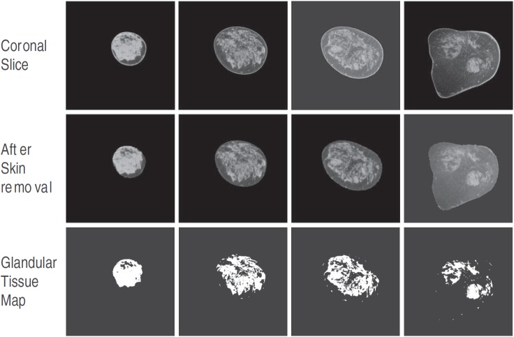
Image preparation steps for estimating the glandular fraction include manually defining the breast volume to be used in the analysis, segmenting the breast from the background (air) region, and segmenting the skin. Briefly, the volume of breast used for analysis was bounded posteriorly to exclude the pectoralis muscle and anteriorly to exclude the areolar region. Segmentation of the breast from the background region^{24, 25} was performed by determining an optimum threshold that was obtained from Gaussian fit to the background voxel intensity. For skin layer segmentation, a method similar to that reported by Huang et al.²⁶ was used, wherein each coronal slice was converted to polar coordinates, followed by application of a 1D derivative filter along the columns to determine the outer and inner boundaries of the skin. The segmented skin layer is removed from the polar transformed slice and converted back to Cartesian coordinates. This procedure is illustrated in Fig. 1.

Figure 1.

Illustration of the process used to prepare the images for segmenting the glandular tissue. From the coronal slice (a), the voxel intensity in the background (air) is sampled and fitted to a Gaussian to obtain an optimal threshold. The breast is segmented from the background and a rectangular region that just includes the breast (b) is generated. The breast (b) is converted to polar coordinates (c) and a first order derivative filter is applied along columns to determine the skin layer (d). The skin layer (d) is subtracted from (c) to provide the breast tissue excluding skin in polar coordinates (e), which is then transformed to Cartesian coordinates (f).

Volumetric glandular fraction

An automated KFCM method was used for classifying each coronal slice that did not include the skin, into two compartments: fibroglandular tissue and adipose tissue. KFCM is adapted from the FCM clustering algorithm, which is an automated and unsupervised technique that has been widely used in medical image segmentation.^{27, 28, 29} Briefly, FCM classifies the image based on its features into desired number of clusters through iteratively minimizing an objective function. A commonly used objective function is the least squares error that uses Euclidean distance (norm) as the metric.²⁹ It has been documented that FCM using Euclidean norm as the metric for an objective function can be affected by outliers (noise) and incomplete data.^{30, 31} Hence, we chose to use a kernel-based FCM method^{31, 32} for fibroglandular tissue segmentation. For this study, we used an open-source program that was available through the MATLAB^® central file exchange.³³ Specific to our study, the image feature space contained only one element, which was voxel intensity, and a Gaussian-kernel based objective function with a Gaussian width σ was used. The value of σ was chosen to be 0.1 for most coronal slices based on visual comparison of the segmented fibroglandular region and the original coronal slice. However, for some coronal slices that exhibited ring artifacts, σ = 0.01 yielded better segmentation. Applying the KFCM algorithm, each coronal slice was partitioned into two clusters based on voxel intensities as either fibroglandular or adipose tissue. For each coronal slice, a binary map representing fibroglandular tissue was generated. Figure 2 illustrates the process for a single breast CT volume where four randomly selected slices are shown. The number of voxels representing fibroglandular and adipose tissue were determined for each coronal slice and summed across all slices to obtain the fibroglandular volume (V_g), the adipose volume (V_a), and hence the total breast volume (TBV = V_g + V_a), after scaling for voxel dimensions. The VGF (Ref. ²³) was determined as $\frac{V_g}{\mathrm{TBV}}$. Thus, our estimate of V_g, TBV, and hence VGF excluded the skin and the areolar region, while the estimate of D_eff was inclusive of skin.

Figure 2.

Four slices selected from a single breast CT volume are shown. The top row contains the coronal slices, the middle row shows the corresponding slices after segmenting and removing the skin, and the bottom row shows the binary maps corresponding to the slices generated using KFCM, where the region representing fibroglandular tissue have a value of 1.

Validation with phantom

The nonuniform spatial distribution of fibroglandular tissue in dedicated breast CT images suggests that the use of an irregular shaped object to represent fibroglandular tissue in a phantom would be preferable. Also, from the average breast volume and mean ± standard deviation of the volumetric breast density reported by Yaffe et al.,¹⁵ the object representing the fibroglandular tissue should have a volume in the range of 24–164 cm³. We are not aware of a commercial phantom that represents an uncompressed breast with a spatial distribution of fibroglandular tissue similar to that observed in breast CT images. Since our objective was to test the algorithm with a complex structure, a phantom comprising a scaled brain aneurysm model fabricated using a 3D prototyping system³⁴ (Prodigy Plus, Stratasys, Eden Prairie, MN) was immersed in a water bath. This phantom was chosen because of its ready availability. The aneurysm volume was physically measured by liquid displacement to be 135.85 cm³, which was considered as “truth.” This value is within the aforementioned range of fibroglandular tissue volume. The phantom was imaged with the dedicated breast CT system using tube current (mA) values that covered the range used in clinical imaging. Figure 3a shows the 3D volume rendering of the phantom and three slices that contain the aneurysm model along with their corresponding binary maps. The KFCM algorithm (σ = 0.1) was applied to segment the aneurysm and its volume was computed.

Figure 3.

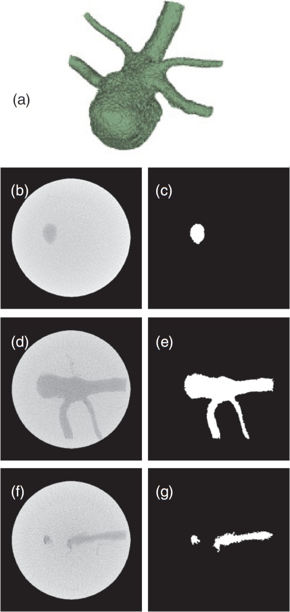
3D volume rendering (a) of the validation phantom comprising an irregular shaped object immersed in water. Selected slices from cone beam CT of the phantom are in the left column (b, d, and f), and their binary images (c, e, and g) where the region within the aneurysm has a value of 1 are in the right column.

Relationship between mammographic breast density and VGF

Mammography-based BI-RADS breast density categories as per the ACR (Ref. ¹⁹) were used to determine its relationship to the quantitative estimates of VGF obtained from breast CT. For clarity, we use the term “mammographic breast density” to represent mammography-based BI-RADS breast density categories. The mammographic breast density categories¹⁹ are: almost entirely fat (<25% fibroglandular tissue); scattered fibroglandular densities (approximately 25%–50% fibroglandular tissue); heterogeneously dense (approximately 51%–75% fibroglandular tissue); and, extremely dense (>75% fibroglandular tissue). For this study, a single radiologist with more than 30 years of experience in breast imaging reviewed the mammograms corresponding to the breasts that were imaged with the breast CT system to provide mammographic breast density assignments and these assignments were used in the analysis.

RESULTS

Validation with phantom

The volume of the scaled aneurysm model measured by liquid displacement was 135.85 cm³ and that determined using KFCM was in the range of 133.33–138.16 cm³, depending on the tube current (mA), indicating that the method was accurate to within ±1.9%. From the segmented regions of the aneurysm and the background (water), the corresponding mean and standard deviation was computed and used to determine the signal-difference-to-noise ratio(SDNR). The SDNR range was 2.6–4.5. A similar procedure was used to compute the SDNR between adipose and fibroglandular tissue in clinical breast CT images. The mean (± standard deviation) SDNR was 11.6 ± 3.9 (range: 7.2–18.9), and in general increased with increasing tube current (mA). This indicates that the chosen phantom represented a more stringent condition in terms of SDNR. The left column of Fig. 3 shows three CT slices selected from the start, middle, and end of the irregular object within the phantom, and the right side shows their corresponding segmented binary images generated using KFCM.

Breast dimensions

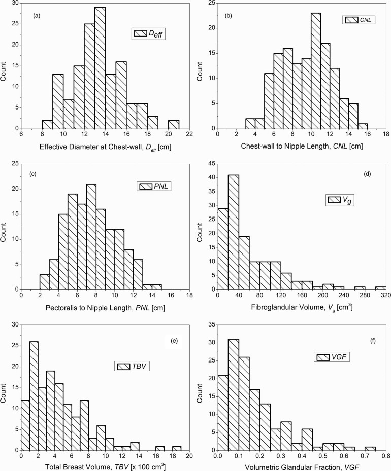
The mean (± inter-breast standard deviation) effective diameter of the breast at the chest-wall inclusive of skin (D_eff) was 13.4 ± 2.4 cm (range: 8.2–20.5 cm). The mean (± inter-breast standard deviation) CNL was 9.5 ± 2.7 cm (range: 3.4–15.2 cm). Summary statistics of these measurements are included in Table 1. The histograms are shown in Fig. 4, where Figs. 4a, 4b, 4c correspond to the effective diameter of the breast at chest-wall (D_eff), CNL, and PNL, respectively. The Spearman's rank correlation coefficient (Spearman rho) was used to assess the correlation between age, CNL, PNL, D_eff, V_g, TBV, and VGF, and is shown in Table 2. Table 2 shows that D_eff, CNL, and PNL were not significantly correlated with age. As expected, there was significant correlation between CNL and PNL, as they are similar measures. There was significant correlation between CNL (and PNL) with D_eff. Figure 5 shows the scatter plot, where CNL is plotted as a function of D_eff. The solid line shows the linear fit with zero-intercept. Current estimates^{35, 36, 37, 38} for normalized glandular dose coefficients (D_gN^CT) assume a linear relationship between CNL and D_eff. The data indicate that the choice of CNL = 0.7014D_eff is suitable, when a linear fit with zero-intercept is assumed. There is a marginal improvement in fit-statistic when a power curve is used to fit the data.

Table 1.

Summary statistics (n = 137) of effective diameter of the breast at chest-wall (D_eff), chest-wall to nipple length (CNL), pectoralis to nipple length (PNL), fibroglandular volume (V_g), total breast volume (TBV), and volumetric glandular fraction (VGF). While D_eff includes the skin, V_g, TBV, and hence VGF exclude the skin and the areolar region.

	Deff	CNL	PNL	Vg	TBV
	(cm)	(cm)	(cm)	(cm3)	(cm3)	VGF
Mean	13.4	9.5	7.6	60.8	453.6	0.172
Inter-breast standard deviation	2.4	2.7	2.6	56.1	338.4	0.142
Lower 95% CI of mean	13.0	9.0	7.1	51.4	396.4	0.148
Upper 95% CI of mean	13.8	9.9	8.0	70.3	510.8	0.196
Minimum	8.2	3.4	2.3	2.1	35.5	0.012
Median	13.3	9.8	7.5	38.8	375.9	0.136
Maximum	20.5	15.2	14.1	301.0	1870.4	0.719
First quartile (Q1)	11.9	7.3	5.5	21.2	193.0	0.067
Third quartile (Q3)	14.7	11.4	9.6	83.4	627.1	0.240

Figure 4.

Histograms of the (a) effective diameter of the breast at chest-wall (D_eff), (b) CNL, (c) PNL, (d) fibroglandular volume (V_g), (e) TBV, and (f) VGF. While D_eff includes the skin, V_g, TBV, and hence VGF exclude the skin and the areolar region.

Table 2.

Correlation (Spearman rho) between age, chest-wall to nipple length (CNL), pectoralis to nipple length (PNL), effective diameter of the breast at chest-wall (D_eff), fibroglandular volume (V_g), total breast volume (TBV), and volumetric glandular fraction (VGF ). While D_eff includes the skin, V_g, TBV, and hence VGF exclude the skin and the areolar region. * indicates significant correlation (two-tailed test) at the 0.05 level.

	Age	CNL	PNL	Deff	Vg	TBV	VGF
Age	1
CNL	0.0136	1
PNL	−0.1056	0.8497*	1
Deff	−0.0291	0.4721*	0.4675*	1
Vg	−0.3124*	0.3896*	0.5059*	0.2208*	1
TBV	−0.0979	0.8098*	0.9406*	0.6112*	0.4800*	1
VGF	−0.2915*	−0.3095*	−0.2870*	−0.3079*	0.5834*	−0.3688*	1

Figure 5.

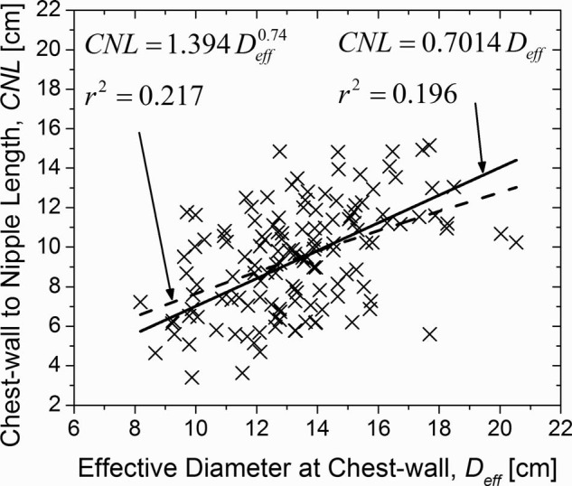
CNL plotted as a function of effective diameter of the breast at chest-wall (D_eff). The linear fit with zero-intercept is provided as current estimates of D_gN^CT assume a similar form. The fit-statistic improves marginally when a power-curve is used to fit the data.

Volumetric measurements

The mean (± inter-breast standard deviation) and the median fibroglandular volume (V_g) were 60.8 ± 56.1 cm³ and 38.8 cm³, respectively (range: 2.1–301 cm³). The mean (± inter-breast standard deviation) and the median TBV were 453.6 ± 338.4 cm³ and 375.9 cm³, respectively (range: 35.5–1870.4 cm³). The large difference between the mean and median for V_g and TBV suggests that the distributions are skewed as shown by the histograms in Figs. 4d, 4e, respectively. Summary statistics are provided in Table 1. While fibroglandular volume (V_g) was significantly correlated with age, TBV was not (Table 2). Also, V_g and TBV were significantly correlated with CNL (and PNL) and D_eff, and there was significant correlation between V_g and TBV (Table 2).

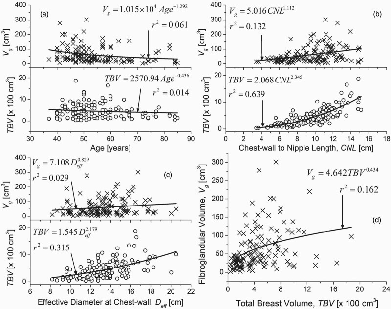
In Fig. 6, the parameters that exhibited significant correlation either with V_g or with TBV are shown. Figures 6a, 6b, 6c show the scatter plots of V_g and TBV as a function of age, CNL and D_eff, respectively. In Fig. 6d, V_g is plotted as a function of TBV. Since the relationship between the parameters plotted in Fig. 6 was not known a priori, a simple allometric power-curve (OriginPro 8.6.0, OriginLab Corporation, Northampton, MA) of the form y = ax^b was used for fitting the data. Although the TBV did not exhibit statistically significant correlation with age, in Fig. 6a, it was observed that the fibroglandular volume (V_g) decreased at a faster rate than TBV with increasing age, as evidenced by the exponents of the corresponding fits. Similarly, based on the exponents of the fits, it can be observed that the TBV increased at a faster rate than V_g with increasing CNL [Fig. 6b] and D_eff [Fig. 6c]. While the fibroglandular volume (V_g) increased with TBV [Fig. 6d], the value for the exponent was less than unity suggesting that the VGF will decrease with increasing TBV, and is addressed below.

Figure 6.

Scatter plots of fibroglandular volume (V_g) and TBV plotted as a function of (a) age of the participant at the time of breast CT exam; (b) CNL; and, (c) effective diameter of the breast at the chest-wall (D_eff). All the aforementioned parameters exhibited significant correlation with either V_g or TBV (Table 2). (d) The scatter plot of V_g as a function of TBV. While D_eff includes the skin, V_g and TBV exclude the skin and the areolar region. All plots were fitted with a simple power curve.

Volumetric glandular fraction

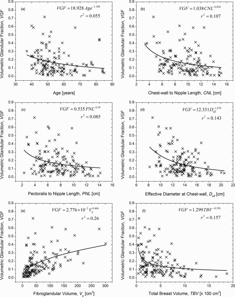
The mean (± inter-breast standard deviation) and the median VGF were 0.172 ± 0.142 and 0.136, respectively (range: 0.012–0.719). Summary statistics are provided in Table 1. The VGF was significantly correlated with age at the time of the breast CT exam, CNL, PNL, D_eff, V_g, and TBV (Table 2). Hence, scatter plots of VGF as a function of aforementioned parameters were plotted and are shown in Fig. 7. A simple allometric power-curve of the form y = ax^b was used to fit the data. With the exception of fibroglandular volume (V_g) shown in Fig. 7e, VGF decreased with an increase in the parameter value consistent with the negative values for the correlation coefficient (Spearman rho) observed in Table 2. The values for the exponent of the power curve provide a direct means to compare the influence of each parameter on the VGF.

Figure 7.

VGF plotted as a function of (a) age at the time of the breast CT exam; (b) CNL; (c) PNL; (d) effective diameter of the breast at chest-wall (D_eff); (e) fibroglandular volume (V_g); and, (f) TBV. All of the plotted parameters exhibited significant correlation with VGF (Table 2). While D_eff includes the skin, V_g, TBV, and hence VGF exclude the skin and the areolar region.

Dependence on race/ethnicity

In our study population, all but nine subjects self-identified themselves as either Whites or African Americans. Hence, we analyzed if any of the metrics studied were dependent on race. Table 3 summarizes the measurements. Mann-Whitney test indicated that the distributions of CNL (p = 3.7E − 4), PNL (p = 5.4E − 5), and TBV(p = 4.9E − 5) were significantly different at the 0.05 level between African Americans and Whites. However, the distributions of D_eff (p = 0.06), V_g (p = 0.09), and VGF (p = 0.08) were not significantly different at the 0.05 level between African Americans and Whites. Figure 8 shows the histograms of CNL, PNL, and TBV that showed statistically significant difference for the distributions.

Table 3.

Summary statistics (n = 128 breasts) showing dependence on race for chest-wall to nipple length (CNL), pectoralis to nipple length (PNL), effective diameter of the breast at chest-wall (D_eff), fibroglandular volume (V_g), total breast volume (TBV), and volumetric glandular fraction (VGF). While D_eff includes the skin, V_g, TBV, and hence VGF exclude the skin and the areolar region. * indicates the two distributions for the corresponding measurement were significantly different at the 0.05 level (Mann-Whitney test).

	CNL*	PNL*	Deff	Vg	TBV*	VGF
African American (n = 35 breasts)
Mean	10.7	9.1	14.0	75.9	649.8	0.134
Standard deviation	2.5	2.6	2.7	66.0	385.3	0.101
Minimum	6.1	3.9	9.2	2.7	82.0	0.012
Median	11.0	9.6	14.3	56.2	688.2	0.121
Maximum	15.2	14.1	20.5	301.0	1870.4	0.414
White (n = 93 breasts)
Mean	8.9	7.0	13.1	56.4	380.7	0.192
Standard deviation	2.6	2.4	2.3	52.3	293.2	0.155
Minimum	3.4	2.3	8.2	2.1	35.5	0.015
Median	9.0	6.9	12.8	36.6	330.8	0.139
Maximum	14.9	13.8	18.5	277.9	1648.8	0.719

Figure 8.

Histograms of CNL, PNL, and total breast volume excluding the skin and the areolar region (TBV) that were significantly different at the 0.05 level between African Americans (AA) and Whites (W).

Dependence on mammographic breast density

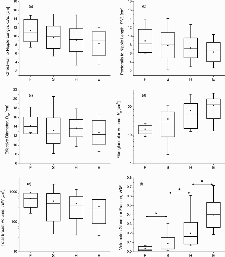
For the 137 breasts analyzed, the mammographic breast density interpretation resulted in assignments of 8 breasts that were almost entirely fat (F), 58 breasts with scattered fibroglandular densities (S), 53 breasts that were heterogeneously dense (H), and 18 breasts that were extremely dense (E). Pairwise comparisons (Mann-Whitney test) of the distributions of VGF in increasing order of mammographic breast density: F vs S (p = 0.002), S vs H (p = 1.3E − 10), and H vs E (p = 9.9E − 8), indicated all comparisons were statistically significant. Figure 9 shows the box-plots between mammographic breast density and the parameters investigated. In all the plots, the symbol and line within the box represent the mean and median, respectively, the box-ends represent ± standard deviation from the mean, and the whiskers represent the minimum and maximum. In terms of the mean, a monotonic decrease with increasing mammographic breast density is observed for the CNL [Fig. 9a], PNL [Fig. 9b], and TBV [Fig. 9e]. The mean estimate of V_g and VGF showed a monotonic increase with increasing mammographic breast density [Figs. 9d, 9e]. Summary statistics of VGF categorized based on mammographic breast density are provided in Table 4.

Figure 9.

Box-plots showing the relationships between mammographic breast density (F – almost entirely fat; S – scattered densities; H – heterogeneously dense; E – extremely dense) and (a) CNL; (b) PNL; (c) effective diameter of the breast at chest-wall (D_eff); (d) fibroglandular volume (V_g); (e) TBV, and (f) VGF. In all plots, the symbol and line within the box represent the mean and median, respectively, the box-ends represent ± standard deviation from the mean, and the whiskers represent the minimum and maximum. (d) and (e) Log-scale for y-axis. In (f), * indicates statistically significant difference between the distributions.

Table 4.

Summary statistics of VGF categorized based on mammographic breast density, where F, S, H, and E represent breasts that were almost entirely fat (F), breasts with scattered fibroglandular densities (S), breasts that were heterogeneously dense (H), and breasts that were extremely dense (E).

	F (n = 8)	S (n = 58)	H (n = 53)	E (n = 18)
Mean	0.036	0.092	0.201	0.399
Standard deviation	0.022	0.062	0.118	0.136
Lower 95% CI of mean	0.017	0.076	0.169	0.332
Upper 95% CI of mean	0.054	0.109	0.234	0.467
Minimum	0.012	0.013	0.065	0.187
Median	0.029	0.074	0.166	0.403
Maximum	0.067	0.308	0.611	0.719
First quartile (Q1)	0.017	0.049	0.135	0.298
Third quartile (Q3)	0.058	0.131	0.247	0.483

Dependence of volumetric glandular fraction on pathology

Pathology results were available for 132 study participants, of which, 38 participants had malignancies (M), 75 had benign findings (B), and 19 had hyperplasia (Hy), of which 11 were atypical. While the mean of VGF was higher for breasts with benign findings and hyperplasia than that for breasts with malignancies (Table 5), pairwise comparisons (Mann-Whitney test) of the distributions of VGF, without adjustment for age, and categorized based on pathology: benign (B) vs hyperplasia (Hy) (p = 0.37); hyperplasia (Hy) vs malignant (M) (p = 0.26); malignant (M) vs benign (B) (p = 0.55); and, by grouping benign and hyperplasia together (B + Hy) vs malignant (M) (p = 0.41), indicated none of the comparisons were statistically significant. Similar pairwise comparisons for the distributions of fibroglandular volume (V_g) and TBV were not statistically significant (p > 0.19).

Table 5.

Summary statistics of VGF categorized based on pathology, where B, Hy, and M indicate that the analyzed breasts had benign findings (B), hyperplasia (Hy), and malignancies (M). B + Hy indicates that the breasts with benign findings and hyperplasia were grouped together.

	B (n = 75)	Hy (n = 19)	B + Hy (n = 94)	M (n = 38)
Mean	0.176	0.189	0.179	0.161
Standard deviation	0.150	0.128	0.145	0.137
Lower 95% CI of mean	0.141	0.128	0.149	0.116
Upper 95% CI of mean	0.210	0.251	0.208	0.206
Minimum	0.012	0.013	0.012	0.015
Median	0.138	0.166	0.140	0.118
Maximum	0.719	0.512	0.719	0.591
First quartile (Q1)	0.069	0.088	0.070	0.067
Third quartile (Q3)	0.241	0.284	0.241	0.240

DISCUSSION

The mean (± inter-breast standard deviation) effective diameter of the breast at the chest-wall inclusive of skin (D_eff) was 13.4 ± 2.4 cm (Table 1), which is in good agreement with physical measurements reported by Boone et al.³⁵ Our estimate of fibroglandular volume (V_g), TBV, and the VGF excluded the skin and the areolar region. For the average dimensions of the breast from this study, D_eff = 13.4 cm and PNL = 7.6 cm (the PNL metric was used for consistency with the study by Yaffe et al.¹⁵), the volume of an average breast assuming a semiellipsoidal shape can be computed as 709.5 cm³, which is good agreement with the previous study.¹⁵

Nelson et al.¹⁴ reported that the percent of fibroglandular tissue within the total breast volume that is inclusive of skin as 17.1% ± 15.2%. Subsequently, Yaffe et al.¹⁵ reported a similar measure of fibroglandular tissue within the total breast volume that is inclusive of skin as 14.3% ± 10.2% by analyzing 191 breast CT exams. In the same study,¹⁵ including mammograms an estimate of 14.3% ± 10.7% was obtained. In comparison, the VGF excluding the skin from this study was 17.2% ± 14.2%. To facilitate direct comparison of our results with the previous studies,^{14, 15} the VGF was recomputed inclusive of the skin, and resulted in mean (± inter-breast standard deviation) of 15.8% ± 13%. Statistical analysis³⁹ (Welch's t-test, two-tailed) indicated that the study results were not statistically different from Nelson et al.¹⁴ (p = 0.48), and Yaffe et al.¹⁵ (p = 0.19).

From Table 2, it is observed that the VGF is negatively correlated with age, breast size (CNL/PNL and D_eff), and TBV and positively correlated with fibroglandular volume (V_g). Since CNL and PNL are similar measures, it is sufficient to consider one of these metrics for analysis. Further, VGF is derived from V_g and TBV. Hence, the dependence of age, CNL and D_eff on V_g and TBV were independently analyzed. In terms of age it is observed from Table 2, that there exists a statistically significant correlation with V_g, but not with TBV. This is also supported by Fig. 6a, where the exponents of the power-curve indicate that V_g decreases at a faster rate than TBV with increasing age, suggesting that the VGF will decrease with increasing age. This observation is confirmed in Fig. 7a.

CNL and D_eff were correlated with V_g and TBV (Table 2). Figures 6b, 6c show the individual effects of CNL and D_eff on V_g and TBV, respectively. Figure 6b shows that both V_g and TBV increase with CNL, with TBV increasing at a faster rate than V_g. Similar observation can also be made for D_eff [Fig. 6c]. In Fig. 7, VGF is observed to decrease with increasing CNL and D_eff, with VGF decreasing at a faster rate for D_eff [Fig. 7d] than CNL [Fig. 7b]. Hence, to understand the combined effects of CNL and D_eff on V_g and TBV, 3D contour plots were generated (OriginPro 8.6.0, OriginLab Corporation, Northampton, MA) and are shown in Fig. 10. In each plot, the levels for the contours were obtained from the quartiles in Table 1. The contours were generated with straight lines connecting the points corresponding to that level. The median of CNL and D_eff are shown, resulting in four quadrants (labeled as Roman numerals I–IV) in each plot. In Fig. 10a, it is observed that subjects with fibroglandular volume (V_g) greater than the third quartile occurred more often in quadrants I and IV, than in quadrants II and III. Comparing quadrants II and IV, it is apparent that more number of subjects with V_g > 3rd quartile occurred in quadrant IV than in quadrant II. These results imply that there is an increase in V_g with increasing CNL and D_eff, and that the increase in V_g is more dependent on CNL than D_eff. These observations are in agreement with the correlation value shown in Table 2, and the value of the exponents shown in Figs. 6b, 6c. In Fig. 10b, it is observed that subjects with TBV greater than the 3rd quartile occurred when CNL and D_eff were greater than their corresponding median. In terms of VGF shown in Fig. 10c, it is observed that all subjects with VGF < 1st quartile had a CNL greater than the median.

Figure 10.

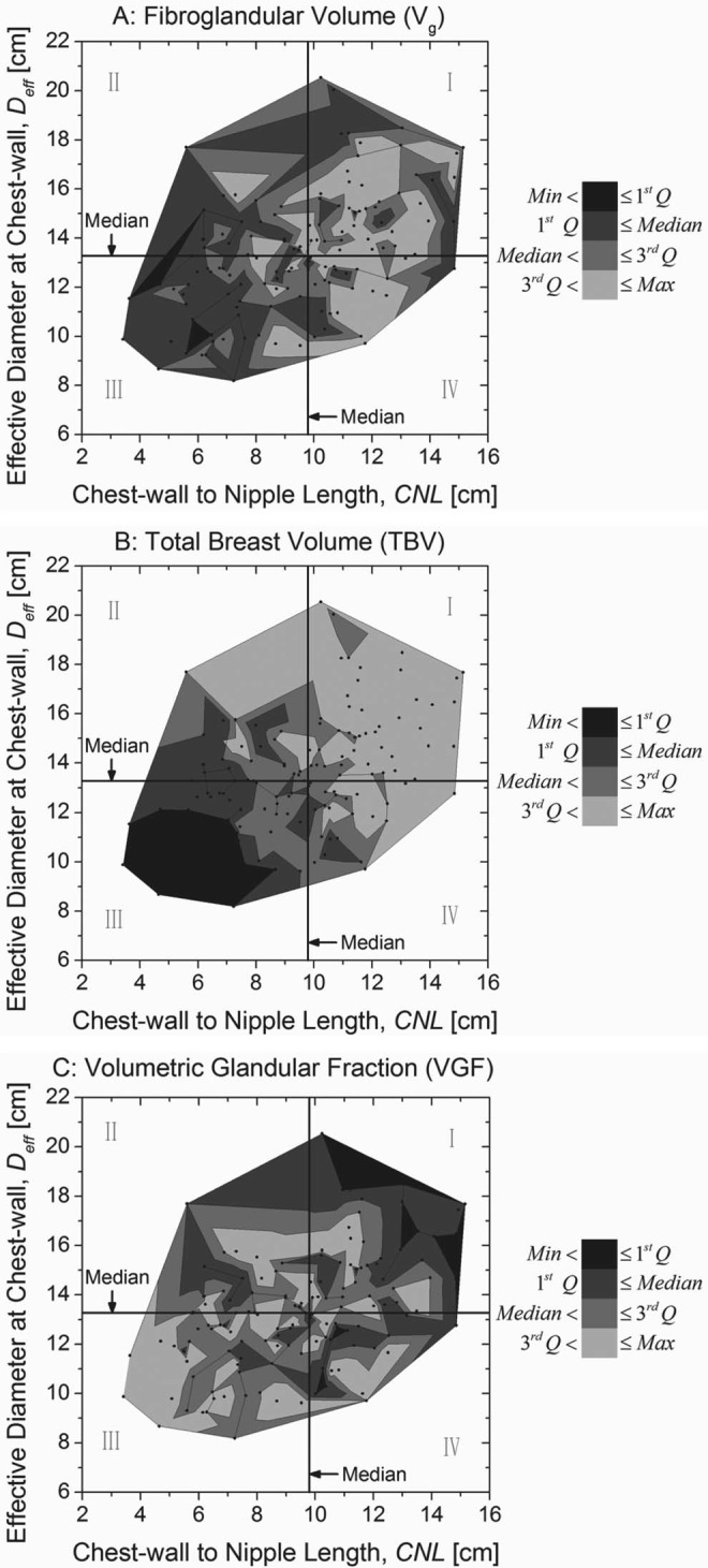
Contour plots were generated to understand the combined effects of CNL and the effective diameter of the breast at chest-wall (D_eff) on (a) fibroglandular volume (V_g), (b) TBV, and (c) VGF. In each plot, the contour levels correspond to the quartiles from Table 1. The median of CNL and D_eff are shown, resulting in four quadrants (labeled as Roman numerals) in each plot.

In terms of race, while the distributions of CNL, PNL, and TBV showed statistically significant differences between African Americans and Whites (p < 3.7E − 4), the distributions of D_eff, V_g, and VGF were not significantly different at the 0.05 level (p > 0.06). A larger study is needed to confirm these findings. Also, pairwise comparisons between malignant and nonmalignant breasts showed that the distributions of V_g, TBV, and VGF were not significantly different at the 0.05 level. This study was not designed to address breast cancer risk; but, to provide a method for determining VGF and to understand the influence of various parameters in the VGF estimate. Since the study only included breast volumes from subjects assigned BI-RADS^® 4 and 5, the study is not suitable for estimating breast cancer risk due to VGF.

Our study had limitations. All breast volumes included in this analysis were from subjects assigned BI-RADS^® 4 and 5, and hence have a suspicious finding. Generally, lesions tend to be segmented as fibroglandular tissue. Hence, V_g and VGF are likely to be overestimated in this study. In 30 of the 137 breast volumes (21.9%), the pectoralis muscle was not imaged. Since, we used PNL=CNL for these cases, the PNL is likely to be underestimated. However, in Table 2 we observe all parameters that exhibit statistically significant correlations with CNL are also significantly correlated with PNL. This suggests it is sufficient to consider one of these parameters, preferably CNL, in future studies.

The data provided here could be useful for Monte Carlo-based estimation of D_gN that are used to estimate the average glandular dose to the breast. Specifically for breast CT, the D_gN^CT coefficients need to be determined for the observed range of CNL and D_eff. In Monte Carlo-based estimation of D_gN, the amount of fibroglandular tissue within the breast is usually specified in terms of glandular weight fraction. Hence, transforming our data that is expressed in volumetric glandular fraction to glandular weight fraction using the method in Boone,⁴⁰ results in a mean of 18.85%. This value is lower than the 50% glandular weight fraction typically used in Monte Carlo based estimates of D_gN used in mammography, indicating that the D_gN factor needs revision.

CONCLUSION

In summary, the mean (± inter-breast standard deviation) VGF excluding the skin and the areolar region was 0.172 ± 0.142. This study used a different clinical prototype breast CT system to image subjects from a different geographical region, and used a different algorithm for analysis of image data. VGF was observed to be dependent on breast dimensions. The distributions of VGF between African Americans and Whites and between malignant and nonmalignant breasts did not vary significantly. Pairwise comparisons of the distributions of VGF in increasing order of mammographic breast density indicated all comparisons were statistically significant.

References

- Wolfe J. N., “Breast patterns as an index of risk for developing breast cancer,” AJR, Am. J. Roentgenol. 126(6), 1130–1137 (1976). [DOI] [PubMed] [Google Scholar]
- Threatt B., Norbeck J. M., Ullman N. S., Kummer R., and Roselle P., “Association between mammographic parenchymal pattern classification and incidence of breast cancer,” Cancer 45(10), 2550–2556 (1980). 10.1002/1097-0142(19800515)45:10<2550::AID-CNCR2820451013>3.0.CO;2-M [DOI] [PubMed] [Google Scholar]
- Boyd N. F., Byng J. W., Jong R. A., Fishell E. K., Little L. E., Miller A. B., Lockwood G. A., Tritchler D. L., and Yaffe M. J., “Quantitative classification of mammographic densities and breast cancer risk: results from the Canadian National Breast Screening Study,” J. Natl. Cancer Inst. 87(9), 670–675 (1995). 10.1093/jnci/87.9.670 [DOI] [PubMed] [Google Scholar]
- McCormack V. A. and dos Santos Silva I., “Breast density and parenchymal patterns as markers of breast cancer risk: A meta-analysis,” Cancer Epidemiol. Biomarkers Prev. 15(6), 1159–1169 (2006). 10.1158/1055-9965.EPI-06-0034 [DOI] [PubMed] [Google Scholar]
- Boyd N. F., Martin L. J., Yaffe M. J., and Minkin S., “Mammographic density and breast cancer risk: Current understanding and future prospects,” Breast Cancer Res. 13(6), 223 (2011). 10.1186/bcr2942 [DOI] [PMC free article] [PubMed] [Google Scholar]
- Byng J. W., Boyd N. F., Fishell E., Jong R. A., and Yaffe M. J., “The quantitative analysis of mammographic densities,” Phys. Med. Biol. 39(10), 1629–1638 (1994). 10.1088/0031-9155/39/10/008 [DOI] [PubMed] [Google Scholar]
- Huo Z., Giger M. L., Wolverton D. E., Zhong W., Cumming S., and Olopade O. I., “Computerized analysis of mammographic parenchymal patterns for breast cancer risk assessment: Feature selection,” Med. Phys. 27(1), 4–12 (2000). 10.1118/1.598851 [DOI] [PubMed] [Google Scholar]
- Boyd N., Martin L., Gunasekara A., Melnichouk O., Maudsley G., Peressotti C., Yaffe M., and Minkin S., “Mammographic density and breast cancer risk: Evaluation of a novel method of measuring breast tissue volumes,” Cancer Epidemiol. Biomarkers Prev. 18(6), 1754–1762 (2009). 10.1158/1055-9965.EPI-09-0107 [DOI] [PubMed] [Google Scholar]
- Glide-Hurst C. K., Duric N., and Littrup P., “A new method for quantitative analysis of mammographic density,” Med. Phys. 34(11), 4491–4498 (2007). 10.1118/1.2789407 [DOI] [PubMed] [Google Scholar]
- Yaffe M. J., “Mammographic density. Measurement of mammographic density,” Breast Cancer Res. 10(3), 209 (2008). 10.1186/bcr2102 [DOI] [PMC free article] [PubMed] [Google Scholar]
- Kopans D. B., “Basic physics and doubts about relationship between mammographically determined tissue density and breast cancer risk,” Radiology 246(2), 348–353 (2008). 10.1148/radiol.2461070309 [DOI] [PubMed] [Google Scholar]
- Wei J., Chan H. P., Helvie M. A., Roubidoux M. A., Sahiner B., Hadjiiski L. M., Zhou C., Paquerault S., Chenevert T., and Goodsitt M. M., “Correlation between mammographic density and volumetric fibroglandular tissue estimated on breast MR images,” Med. Phys. 31(4), 933–942 (2004). 10.1118/1.1668512 [DOI] [PubMed] [Google Scholar]
- Chang D. H., Chen J. H., Lin M., Bahri S., Yu H. J., Mehta R. S., Nie K., Hsiang D. J., Nalcioglu O., and Su M. Y., “Comparison of breast density measured on MR images acquired using fat-suppressed versus nonfat-suppressed sequences,” Med. Phys. 38(11), 5961–5968 (2011). 10.1118/1.3646756 [DOI] [PMC free article] [PubMed] [Google Scholar]
- Nelson T. R., Cervino L. I., Boone J. M., and Lindfors K. K., “Classification of breast computed tomography data,” Med. Phys. 35(3), 1078–1086 (2008). 10.1118/1.2839439 [DOI] [PMC free article] [PubMed] [Google Scholar]
- Yaffe M. J., Boone J. M., Packard N., Alonzo-Proulx O., Huang S. Y., Peressotti C. L., Al-Mayah A., and Brock K., “The myth of the 50-50 breast,” Med. Phys. 36(12), 5437–5443 (2009). 10.1118/1.3250863 [DOI] [PMC free article] [PubMed] [Google Scholar]
- Glide-Hurst C. K., Duric N., and Littrup P., “Volumetric breast density evaluation from ultrasound tomography images,” Med. Phys. 35(9), 3988–3997 (2008). 10.1118/1.2964092 [DOI] [PubMed] [Google Scholar]
- FDA U. S., “Mammography Quality Standards Act Regulations. Sec. 900.12 Quality standards.(e) Quality assurance-equipment (5) Annual quality control tests,” U.S. Food and Drug Administration, Rockville, MD, 2002. (http://www.fda.gov/Radiation-EmittingProducts/MammographyQualityStandardsActandProgram/Regulations/ucm110906.htm#s90012).
- ACR, Mammography Quality Control Manual (American College of Radiology (ACR), Reston, VA, 1999). [Google Scholar]
- ACR, Breast Imaging Reporting and Data System, Breast Imaging Atlas, 4th ed. (American College of Radiology (ACR), Reston, VA, 2004). [Google Scholar]
- Benitez R. B., Ning R., Conover D., and Liu S. H., “NPS characterization and evaluation of a cone beam CT breast imaging system,” J. X-Ray Sci. Technol. 17(1), 17–40 (2009). 10.3233/XST-2009-0213 [DOI] [PubMed] [Google Scholar]
- O’Connell A., Conover D. L., Zhang Y., Seifert P., Logan-Young W., Lin C. F., Sahler L., and Ning R., “Cone-beam CT for breast imaging: Radiation dose, breast coverage, and image quality,” AJR, Am. J. Roentgenol. 195(2), 496–509 (2010). 10.2214/AJR.08.1017 [DOI] [PubMed] [Google Scholar]
- Feldkamp L. A., Davis L. C., and Kress J. W., “Practical cone-beam algorithm,” J. Opt. Soc. Am. A 1(6), 612–619 (1984). 10.1364/JOSAA.1.000612 [DOI] [Google Scholar]
- Huang S. Y., Boone J. M., Yang K., Packard N. J., McKenney S. E., Prionas N. D., Lindfors K. K., and Yaffe M. J., “The characterization of breast anatomical metrics using dedicated breast CT,” Med. Phys. 38(4), 2180–2191 (2011). 10.1118/1.3567147 [DOI] [PMC free article] [PubMed] [Google Scholar]
- Brummer M. E., Mersereau R. M., Eisner R. L., and Lewine R. J., “Automatic detection of brain contours in MRI data sets,” IEEE Trans. Med. Imaging 12(2), 153–166 (1993). 10.1109/42.232244 [DOI] [PubMed] [Google Scholar]
- Atkins M. S. and Mackiewich B. T., “Fully automatic segmentation of the brain in MRI,” IEEE Trans. Med. Imaging 17(1), 98–107 (1998). 10.1109/42.668699 [DOI] [PubMed] [Google Scholar]
- Huang S. Y., Boone J. M., Yang K., Kwan A. L., and Packard N. J., “The effect of skin thickness determined using breast CT on mammographic dosimetry,” Med. Phys. 35(4), 1199–1206 (2008). 10.1118/1.2841938 [DOI] [PMC free article] [PubMed] [Google Scholar]
- Pham D. L., Xu C., and Prince J. L., “Current methods in medical image segmentation,” Annu. Rev. Biomed. Eng. 2, 315–337 (2000). 10.1146/annurev.bioeng.2.1.315 [DOI] [PubMed] [Google Scholar]
- Bezdek J. C., Keller J., Krisnapuram R., and Pal N. R., Fuzzy Models and Algorithms for Pattern Recognition and Image Processing (Springer Science+Business Media, Inc., New York, NY, 2005). [Google Scholar]
- Chen W., Giger M. L., and Bick U., “A fuzzy c-means (FCM)-based approach for computerized segmentation of breast lesions in dynamic contrast-enhanced MR images,” Acad. Radiol. 13(1), 63–72 (2006). 10.1016/j.acra.2005.08.035 [DOI] [PubMed] [Google Scholar]
- Wu K. L. and Yang M. S., “Alternative c-means clustering algorithms,” Pattern Recogn. 35(10), 2267–2278 (2002). 10.1016/S0031-3203(01)00197-2 [DOI] [Google Scholar]
- Zhang D. Q. and Chen S. C., “Clustering incomplete data using kernel-based fuzzy C-means algorithm,” Neural Process. Lett. 18(3), 155–162 (2003). 10.1023/B:NEPL.0000011135.19145.1b [DOI] [Google Scholar]
- Hathaway R. J., Huband J. M., and Bezdek J. C., “Kernelized non-Euclidean relational fuzzy c-means algorithm,” Proceedings of the 14th IEEE International Conference on Fuzzy Systems, FUZZ'05, Reno, NV (IEEE, 2005), pp. 414–419. 10.1109/FUZZY.2005.1452429 [DOI]
- Rong G., “A GUI about medicinal images segmentation with FCM or KFCM (Kernelled FCM),” (http://www.mathworks.com/matlabcentral/fileexchange/9165-a-gui-about-medicinal-images-segmentation-with-fcm-or-kfcmkernelled-fcm, 2005)
- Chueh J. Y., Wakhloo A. K., and Gounis M. J., “Neurovascular modeling: Small-batch manufacturing of silicone vascular replicas,” AJNR Am. J. Neuroradiol. 30(6), 1159–1164 (2009). 10.3174/ajnr.A1543 [DOI] [PMC free article] [PubMed] [Google Scholar]
- Boone J. M., Shah N., and Nelson T. R., “A comprehensive analysis of DgN(CT) coefficients for pendant-geometry cone-beam breast computed tomography,” Med. Phys. 31(2), 226–235 (2004). 10.1118/1.1636571 [DOI] [PubMed] [Google Scholar]
- Thacker S. C. and Glick S. J., “Normalized glandular dose (DgN) coefficients for flat-panel CT breast imaging,” Phys. Med. Biol. 49(24), 5433–5444 (2004). 10.1088/0031-9155/49/24/003 [DOI] [PubMed] [Google Scholar]
- Sechopoulos I., Feng S. S., and D’Orsi C. J., “Dosimetric characterization of a dedicated breast computed tomography clinical prototype,” Med. Phys. 37(8), 4110–4120 (2010). 10.1118/1.3457331 [DOI] [PMC free article] [PubMed] [Google Scholar]
- Vedantham S., Shi L., Karellas A., and Noo F., “Dedicated breast CT: Radiation dose for circle-plus-line trajectory,” Med. Phys. 39(3), 1530–1541 (2012). 10.1118/1.3688197 [DOI] [PMC free article] [PubMed] [Google Scholar]
- “QuickCalcs - t test calculator” (GraphPad Software Inc., La Jolla, CA, 2012, http://graphpad.com/quickcalcs/ttest1/?Format=SD).
- Boone J. M., “Glandular breast dose for monoenergetic and high-energy x-ray beams: Monte Carlo assessment,” Radiology 213(1), 23–37 (1999). [DOI] [PubMed] [Google Scholar]