OpenMx: An Open Source Extended Structural Equation Modeling Framework

Abstract

OpenMx is free, full–featured, open source, structural equation modeling (SEM) software. OpenMx runs within the R statistical programming environment on Windows, Mac OS–X, and Linux computers. The rationale for developing OpenMx is discussed along with the philosophy behind the user interface. The OpenMx data structures are introduced — these novel structures define the user interface framework and provide new opportunities for model specification. Two short example scripts for the specification and fitting of a confirmatory factor model are next presented. We end with an abbreviated list of modeling applications available in OpenMx 1.0 and a discussion of directions for future development.

Structural Equation Modeling: Context and Motivation

Structural equation modeling has a long history dating back to the development of path analysis by Sewall Wright (Wright, 1921). Path analysis is an algorithmic tool for deriving a set of predicted covariances between variables which may be connected with either regression (asymmetric, directional) or correlation (symmetric, non-directional) paths. The advent of high speed computers and high level programming languages in the 1960's, together with advances in statistical methodology (Jöreskog, 1967) led to the development of software for fitting models to observed covariance matrices by maximum likelihood. This procedure is now commonly known as structural equation modeling (SEM). Several extensions of this methodology have increased its scope: modeling of means as well as covariances (Sörbom, 1974); specifying certain paths as observed variables (known as definition variables in Mx) (Neale, 1998; Neale, Boker, Xie, & Maes, 2006)); and fitting finite mixture distributions (Eaves, Neale, & Maes, 1996; Everitt & Hand, 1981; McLachlan & Peel, 2000).

A search of the PsycInfo database for “latent variable” or “latent class” or “structural equation model” gives an estimate of the increasing popularity of SEM: 1970's, 23; 1980's, 357; 1990's, 2,794; and 2000-2009, 9,599. These searches underestimate the actual number of published articles that used this method, as many abstracts do not provide detail about the statistical methods used. At the same time, the great variety of statistical methods that are subsumed by SEM including analysis of variance, multiple regression, discriminant analysis, canonical and partial correlations, factor analysis, principal components analysis and multilevel analysis, (Marcoulides & Schumacker, 1996; McArdle & Hamagami, 1996; Longford & Muthén, 1992) further demonstrate its broad utility.

The increased popularity of SEM has been accompanied by two changes in the statistical analysis of research data. First is that the complexity of the models and methods being used has increased dramatically. In statistical modeling, problems that were previously regarded as impossibly complex have become regarded as tractable. This trend is partly driven by Moore's Law, which states that the complexity of computer circuits (i.e., computing power) doubles approximately every 18-24 months (Moore, 1965). Both methodological and substantive researchers have sought to exploit developments in computer architecture with statistical methods to improve the quality of their scientific output.

The second change is that as data collection methods have become more automated and data storage has become inexpensive, datasets have dramatically increased in size. As a result, research projects have become more ambitious, collecting many measurements from large samples of subjects. SEM, which has made possible a range of complex analyses, has the potential to be an extremely valuable approach to these new challenges due to i) greater statistical power (less variance in study outcomes), and ii) greater precision (less bias in the results).

There is a wide variety of software that allows the estimation of SEM models. Examples include Amos (Arbuckle, 2009), Calis (PROC CALIS, 2009), EQS (Bentler, 2009), LISREL (Jöreskog & Sörbom, 2009), Mplus (Muthén & Muthén, 2009), Mx (Neale et al., 2006), RAMONA (Browne & Mels, 2009), sem (Fox, 2009), and SEPath (SEPath, 2009). Given this crowded field of SEM software, it is perhaps surprising that there might be room for a new SEM package. The present article announces the availability of new SEM software that is substantially different from that currently available. We believe that OpenMx fills an open evolutionary niche in the extant SEM software ecology.

Why a New SEM Package?

OpenMx is a free, open source, full–featured SEM package that runs inside the R statistical programming environment (Ihaka & Gentleman, 1996). Although the programming team includes authors of the original Mx software, OpenMx has been rewritten from scratch using modern languages and programming techniques. Model specification has been redesigned to be much more flexible and general than that used by traditional SEM software.

Open Source

OpenMx is open source; thus the source code is available for everyone to view, modify, and use. We currently have a team of dedicated programmers and a design team determining the direction of OpenMx. The project itself is organized somewhat like a scientific journal: Code can be submitted for review by the “editorial board” who read, edit, and test the code. Code that is accepted for publication as part of the OpenMx package becomes available for the entire scientific community. We do not place any limits on how readers and users of the code may use the software and code, but we do expect that code that is part of OpenMx is cited by people who use it. Authors who contribute code are cited by the project and by others who use their code.

In order to help organize an open source community, the OpenMx project maintains a web site (http://openmx.psyc.virginia.edu) that hosts binary and source versions of the software and several forms of tutorials and reference documentation. On the web site, a set of open–access forums have been established to allow the SEM community a place to discuss SEM models, theory, and methodology. In addition, help on OpenMx is available on the web site from discussion forums and a community–maintained Wiki. Finally, a set of developer forums is also hosted in order to allow statistical programmers a place to communicate about new ideas and patches that may become part of the base OpenMx project.

Sustainability

OpenMx has been written using modular programming techniques in the C and R languages with the intent that it will be maintained and extended by members of the research community. Modular programming design means that the code is written so that each section of code operates independently and is accessed via a well–defined interface. This means that many programmers can be working on the code simultaneously as long as each module of code maintains the expected behavior from its interface. In order to work on part of OpenMx, one does not need to understand the inner workings of all other modules; it is only necessary to understand and adhere to the interface specifics for that specific module.

The core programming team is working hard to encourage and help statistical and quantitative researchers to add their research projects to the larger OpenMx SEM framework. For instance, someone who is working on a particular type of estimation, a particular type of model, or perhaps a new fit statistic can incorporate his or her research into a project that is immediately available to a large community of users. One does not need to write model specification methods, input/output methods, data handling methods, and all the other parts required before substantive researchers can use the novel software. We expect that the user interface, estimation methods, and reporting functions for OpenMx will evolve quickly due to the influx of new ideas and code contributed by the large community of SEM users.

Rethinking Model Specification and Estimation

SEM models are becoming more difficult to specify and estimate as substantive theory and data grow increasingly complex. Massive data sets including genome–wide association and brain imaging are at the leading edge of this evolving research landscape. These data sets are many orders of magnitude larger than those available when most SEM software was originally designed and programmed. For instance, an fMRI data set might include 40,000 voxels per frame per person. An SEM model of these data might include hundreds of latent variables and tens of thousands of free parameters. In such a case, one would need a large parallel computing grid to estimate the model. OpenMx has been designed from the beginning with parallel computing in mind, both for use with multicore computers and with very large grids of computers such as the TeraGrid and Open Science Grid.

Heterogeneous Computing Environments

OpenMx runs on a variety of operating systems including Microsoft Windows, Mac OS-X, and most popular variants of Linux. OpenMx scripts that are written within one operating system can be used on other operating systems without modification. This platform–independence is useful in today's heterogeneous computing environments where each researcher on a team may have a different preferred computing platform. In addition, this multi–platform support means that heterogeneous grids of computers can be used to run OpenMx, a common occurrence in parallel distributed computing environments.

A New Approach to Model Specification

Two methods are currently in use for specifying SEM models in scripts. The first centers around specifying the matrices that define the covariance and mean structure of the manifest and latent variables. The second method is based on path analysis and uses a compact specification for the paths and variables in a path diagram. In the end, both of these methods produce a set of matrix equations that are used as an objective function (sometimes called a cost function) that is optimized in order to find parameters such that the objective function is at a minimum. Popular objective functions include maximum likelihood and several variants of least squares.

OpenMx implements both matrix–centric and path–centric methods for specifying the desired structure of the model. Thus, one can use either of these two methods or even a combination of the two. We will provide a short example of these two methods later in the article. In addition to providing built–in objective functions such as FIML, OpenMx provides methods for the user to specify their own custom objective functions.

The data structures that are produced when one creates an OpenMx SEM model are a departure from the structures produced by other SEM software. We will next describe these structures and how they fit together. While software has improved, SEM modelers continue to think about their model structure in ways that have changed very little since the 1960s. One may use OpenMx without changing one's conception of model building, continuing to use path specifications or matrix specifications in a serially ordered script. However, the fact that R is interactive, has powerful vector and matrix operations, and incorporates the flow control of a full programming language all act to allow one to rethink the way models are specified. The OpenMx data structures are designed to flexibly accommodate the power of R. The authors hope that these factors will be sufficient to trigger a paradigm shift in the way SEM is conceived and taught.

This section begins with a description of three of the basic structures in OpenMx: MxModel, MxMatrix, and MxAlgebra. We describe how MxModels may contain other Mx-Models in a tree–like hierarchy, and how references are made within an MxModel hierarchy. We then briefly discuss how data and objective functions are specified within an MxModel. Finally, we provide two example specifications of a simple confirmatory factor model.

MxModels and the Objects They Contain

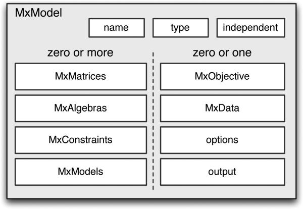
Data structures in OpenMx are implemented as objects, specifically R S4 objects. The MxModel is the object that contains all of what is necessary in order to specify a structural model. It is primarily a container for other objects while providing the organization that allows the contained objects to refer to one another (see Figure 1). Each MxModel has three slots for metainformation about the model: an internal reference name, a type, and a flag that indicates whether the model can be estimated independently from other models.

Figure 1.

An MxModel is a data object that contains metainformation and lists of other Mx objects.

MxModels define a namespace, in other words, a self–contained set of strings that define either (1) objects or (2) elements in matrices. Each of these names is unique within the namespace. Therefore, if a name occurs more than once during the specification of an MxModel, it is taken to mean that the name is referring to the same thing. This turns out to be very powerful. For instance, if you name two matrix elements “b” then these two elements are constrained to be equal.

An MxModel may contain: lists of MxMatrices, MxAlgebras, MxConstraints, no more than one MxData object, and an objective function. There are also slots in the MxModel that contain a list of optimization options and a list that contains output from the most recent optimization run. We note here that MxModels can also contain a list of other MxModels. This allows one to create a hierarchical tree of MxModels which is subsumed within a root MxModel container. A hierarchical tree of child and parent MxModels provides a new way of thinking about constructing SEM models that is surprisingly powerful.

An MxMatrix is an object which contains five separate R matrices and five metainformation slots: a type, the number of rows and columns; the labels for each row and column (in R this is called dimnames); and the name by which the matrix is known in its MxModel namespace. The five matrices in the MxMatrix are all of the same order, but of different R storage types. The values matrix holds the starting (or estimated) values and is of type double. The labels matrix is of type character and holds the name of each element of the matrix. Matrix elements that have the same name are constrained to be equal to one another. The free matrix is of type logical and if an element is TRUE, then that element is considered to be a free parameter during estimation. The lbound and ubound matrices are of type double and contain lower and upper bounds for the free parameters.

An MxAlgebra is an object that contains its name, a formula in R notation, and a result matrix of type double. The operands in the formula are named objects in the MxModel namespace that are either an MxMatrix or an MxAlgebra. Matrix operators include most of the common matrix operations such as addition, subtraction, matrix multiplication, dot product, Kronecker product, inverse, transpose, augmentation, exponentiation, log, and many others. A full list of operators can be found on the OpenMx website wiki.

An MxConstraint contains two objects, either of which can be an MxMatrix or MxAlgebra, and a relation between them, which can be one of >, <, or ==. This allows the specification of nonlinear constraints which should be satisfied at the end of optimization.

Objective Functions and Data

One of the most flexible parts of OpenMx is the way that the objective functions can be defined. An objective function for optimization results in a scalar number that is minimized. Examples of predefined objective functions include maximum likelihood (mxMLObjective) and full information maximum likelihood (mxFIMLObjective). However, other objective functions can be specified using the mxAlgebraObjective which allows one to specify a formula in the same way as an MxAlgebra is specified with the caveat that the result of the formula must be a 1 × 1 matrix. This allows the possibility of creating objective functions that perform specific optimizations such as variants of least squares or even various Bayesian optimizations.

The MxData object contains the data used for optimization. The data object may be raw data, a correlation matrix, a covariance matrix, a covariance matrix and vector of means, or a sums of squares and crossproducts matrix. Each column in the raw data or covariance matrix must have a column name. If the data is an R dataframe or covariance matrix calculated from a dataframe, these column names are automatically supplied, but these column names must be defined via dimnames for data supplied from other sources. Named columns in MxMatrices that match the dimnames in the MxData are automatically mapped to the correct column in the data.

MxModel Trees

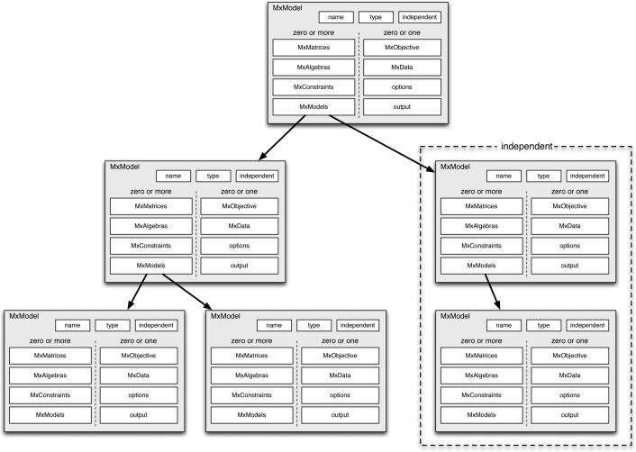
One of the novel features of OpenMx is that models can contain other models as shown in Figure 3. This allows one to think very naturally about how dependency is structured in an SEM context. For instance, a model hierarchy can be built that expresses dependency in a genetic SEM analysis: An ACE model is built that contains matrices common to all groups and then two submodels are constructed, one for the monozygotic twin pairs and one for the dizygotic twin pairs. This approach partitions the problem into submodels that follow the logical group structure in the data. A Mixture distribution analysis can be set up as a model tree where the submodels are the elements of the mixture and the top level model expresses the overall likelihood calculation for the mixture.

Figure 3.

MxModels can contain lists of submodels.

Multiple independent models can be grouped together as submodels into a single run for problems such as bootstrapping or simulations where the top level model can fit an overall model on the estimation results returned from the independent models. In a case of independent models, OpenMx uses the facilities of snow and swift to distribute the job over multiple CPUs The limit to how many models can be structured into a hierarchy is the memory limit of your computer. We have run cases with tens of thousands of submodels.

A model hierarchy structure allows one to express the logic of an analysis in a straightforward and simplified manner. This feature of OpenMx is a departure from traditional SEM specification, and has proven popular among beta testers of OpenMx.

References within MxModels and MxModel Trees

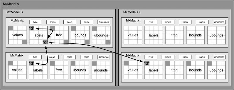
The namespace for an MxModel includes all of the non–independent models in a hierarchical tree. Thus, for instance, parameters can be constrained between two submodels as shown in Figure 4. Constraints cannot be made to elements in an independent submodel — one of the conditions that allows independent estimation of branches of a model tree that have been marked as independent. In Figure 4 four elements from three matrices across two submodels have all been constrained to be equal by labeling the corresponding elements as “d”.

Figure 4.

Equality constraints can be defined between submodels.

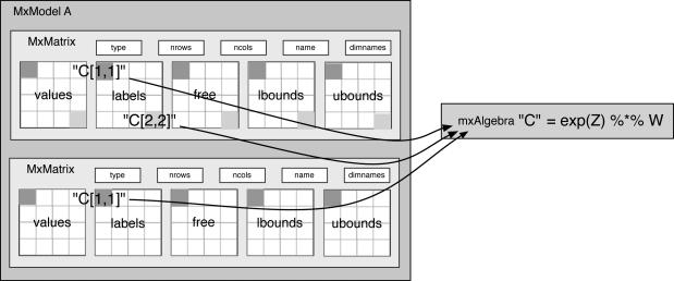
Free elements of MxMatrices can also be constrained to be equal to the results of MxAlgebras by using labels that include the MxAlgebra name and an index into the result matrix of the MxAlgebra as shown in Figure 5. This allows matrix elements to be constrained to be nonlinear functions of free parameters for use in, e.g., logistic regression or continuous time differential equations models.

Figure 5.

Labels can be used to constrain a matrix element to be equal to a matrix element from an algebraic result.

Example Scripts

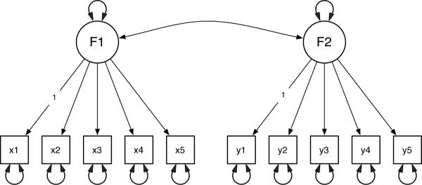
In order to give an introduction to how OpenMx scripts are written, we present a confirmatory two factor model with simple structure as shown in Figure 6. The model will be specified using two methods.

Figure 6.

A simple confirmatory factor analysis model as a RAM–style path diagram.

Path Analysis Method

First, we will use the path analysis method to specify the model. In this approach, we first define the variables and then specify the regression, variance, and covariance paths. While this method is verbose, it is designed to expose all of the parts of the model. Hiding functionality behind defaults allows a script to be shorter to type, but it can mean that it is difficult to understand exactly what the model does (the “Black Box” problem). By making all parts of the model specification explicit, we expose all of the model to inspection. We have found that this philosophy results in scripts that are easier for i) students to learn and ii) others to understand.

# load the OpenMx package into R
library(OpenMx)
# read the data into an R dataframe
factorData <- read.csv(“demoTwoFactor.csv”)
# define which indicators load on each factor
indicatorsF1 <- c(“x1”, “x2”, “x3”, “x4”, “x5”)
indicatorsF2 <- c(“y1”, “y2”, “y3”, “y4”, “y5”)
# create a vector of all of the manifest variables
manifests <- c(indicatorsF1, indicatorsF2)
# define which indicator is to be used to scale each factor
scaleF1 <- c(“x1”)
scaleF2 <- c(“y1”)
# define the names of the factors
latents <- c(“F1”, “F2”)
# define the MxModel and store it into “factorModel“
factorModel <- mxModel(“Simple Structure Two Factor”,
type=“RAM”,
manifestVars = manifests,
latentVars = latents,
# specify the free factor loadings
mxPath(from=“F1”, to=indicatorsF1, free=TRUE, values=.2),
mxPath(from=“F2”, to=indicatorsF2, free=TRUE, values=.2),
# scale the two latent variables
mxPath(from=“F1”, to=scaleF1, free=FALSE, values=1),
mxPath(from=“F2”, to=scaleF2, free=FALSE, values=1),
# specify the unique variances
mxPath(from=manifests, arrows=2, free=TRUE, values=.8),
# specify the factor variances
mxPath(from=latents, arrows=2, free=TRUE, values=.8),
# specify the factor covariance
mxPath(from=“F1”, to=“F2”, arrows=2, free=TRUE, values=.3),
# specify the mean structure
mxPath(from=“one”, to=c(manifests, latents), arrows=1, free=FALSE, values=0),
# attach the data to the model
mxData(factorData, type=“raw”) )
# run the factor model
factorModelOut <- mxRun(factorModel)
# print a summary of the results
summary(factorModelOut)

Note that we find it convenient to first set up vectors of character strings that define which indicators are used with which factors and which indicators are used to scale the factors by fixing their values to 1.0. This allows us to use shorthand to create many loading paths at once in the mxPath statements — whenever there is a vector of “from variables” or “to variables”, the mxPath function creates all of the connections at once.

Matrix Method

While the path analysis method may be preferred for some models, it is often either easier or is necessary to use matrices to specify a model. Many of the advanced models available in OpenMx have no equivalent path diagram and so their covariance algebra must be specified via matrices. In addition, matrix specification is frequently more compact than specifying all of the paths.

We will respecify the model in Figure 6 as a product of matrices. This model is of factor analytic form and so the expected covariance matrix of the indicators, R, can be written as

$$\mathbf{R}={\mathbf{ALA}}^{\prime }+\mathbf{U},$$ (1)

where A is the matrix of factor loadings, L is the factor intercorrelation matrix, and U is the diagonal matrix of unique factor variances. This model can be written in OpenMx using the following script.

# load the OpenMx package into R
library(OpenMx)
# read the data into an R dataframe
factorData <- read.csv(“demoTwoFactor.csv”)
# read the names of the indicator variables from the dataframe
indicators <- names(factorData)
# define the MxModel and store it into “factorModel”
factorModel <- mxModel(“One Factor”,
# specify the loading matrix including its starting values and which elements are free mxMatrix(“Full”, nrow=10, ncol=2, values=c(1,rep(0.2,4),rep(0,10),1,rep(0.2,4)), free=c(FALSE,rep(TRUE,4),rep(FALSE,10),FALSE,rep(TRUE,4)), name=“A”),
# specify the factor intercorrelation matrix
mxMatrix(“Symm”, nrow=2, ncol=2, values=.8, free=T, name=“L”),
# specify the matrix of unique factor variances
mxMatrix(“Diag”, nrow=10, ncol=10, values=1, free=T, name=“U”),
# specify the algebra that results in the model expectations
mxAlgebra(A %*% L %*% t(A) + U, dimnames = list(indicators, indicators), name=“R” ),
# specify a model for the means fixed at zero
mxMatrix(“Full”, nrow=1, ncol=10, values=0, free=FALSE, dimnames=list(NULL, indicators), name=“M” ),
# choose the full information maximum likelihood objective function
mxFIMLObjective(covariance=“R”, means=“M”),
# attach the data to the model
mxData(factorData, type=“raw”) )
# run the factor model
factorModelOut <- mxRun(factorModel)
# print a summary of the results
summary(factorModelOut)

The trickiest part of this version of the script is the way that the loading matrix, A, is specified. Note that R stores values into matrices column–wise unless byrow=TRUE is selected. So, the matrix A ends up as a 10 × 2 matrix with starting values

$$\mathbf{A}=\left[\begin{array}{cc}\hfill 1.0& \hfill 0\\ \hfill 0.2& \hfill 0\\ \hfill 0.2& \hfill 0\\ \hfill 0.2& \hfill 0\\ \hfill 0.2& \hfill 0\\ \hfill 0& \hfill 1.0\\ \hfill 0& \hfill 0.2\\ \hfill 0& \hfill 0.2\\ \hfill 0& \hfill 0.2\\ \hfill 0& \hfill 0.2\end{array}\right]$$ (2)

If you look carefully in the script above at the values= line in the specification of the matrix A, you can see how the values from vector are stored into the A matrix. A similar method is used to specify which loadings are fixed and which are to be estimated in the matrix A. All elements with starting values of 0.2 end up designated as free=TRUE whereas all others are designated as free=FALSE.

Other Specification Styles

Since R is a full programming language and the OpenMx specification structure is flexible, there are many styles of model specification that could be used to create identical statistical models. We expect several styles will emerge as users become acquainted with the possibilities. One style that has become common among the core programming team members is to specify each of the MxMatrices separately, assigning them to R variables early in a script. Later, these predefined matrices can be combined into different model configurations somewhat like using Lego blocks. This method results in scripts that bear little resemblance to traditional SEM scripts, but these Lego–style scripts can be easier to write, debug, and maintain.

Summary

The OpenMx project is full–featured, open source, SEM software that runs on most available operating systems. The software runs in the R statistical computing environment. The user interface is designed to be: i) flexible in that there are many ways in which models can be defined; ii) powerful in that models can be specified without relying on hidden mechanisms; and iii) extensible in that there are facilities to add new objective functions and optimization methods.

A wide variety of SEM models can be fit with OpenMx. A few of the more popular models that are in current use include: confirmatory factor analysis, multivariate autoregression with cross–lags, latent growth curves, latent mediation, multivariate mixed e ects, multigroup models with constraints, behavioral genetic and genetic epidemiological models, multivariate ordinal models with threshold estimation, factor mixture models, latent differential equations, latent class models. All of these models can be (and sometimes must be) run using full information maximum likelihood estimation.

When independent submodels are specified, OpenMx allows for automatic use of multiple CPUs in modern multicore systems. When a computer cluster or distributed grid of computers is available, OpenMx can take advantage of this service to run its independent submodels on multiple computers simultaneously.

The current article only briefly covers the many features and facilities of OpenMx. To learn more, obtain a free download of the software, and participate in the OpenSEM forums please go to http://openmx.psyc.virginia.edu.

Figure 2.

An MxMatrix is a data object that contains metainformation and five R matrices.

References

- Arbuckle JL. Amos user's guide. SPSS; Chicago: 2009. [Google Scholar]
- Bentler PM. EQS structural equations program manual. Multivariate Software; Encino, CA: 2009. [Google Scholar]
- Browne MW, Mels G. RAMONA: SYSTAT for Windows. SYSTAT; 2009. [Google Scholar]
- Eaves LJ, Neale MC, Maes HH. Multivariate multipoint linkage analysis of quantitative trait loci. Behavior Genetics. 1996;26:519–526. doi: 10.1007/BF02359757. [DOI] [PubMed] [Google Scholar]
- Everitt BS, Hand DJ. Finite mixture distributions. Chapman and Hall; 1981. [Google Scholar]
- Fox J. sem: Structural Equation Models. (R package version 0.9–19) 2009.
- Ihaka R, Gentleman R. R: A language for data analysis and graphics. Journal of Computational and Graphical Statistics. 1996;5(3):299–314. [Google Scholar]
- Jöreskog KG. Some contributions to maximum likelihood factor analysis. Psychometrika. 1967;32:443–482. [Google Scholar]
- Jöreskog KG, Sörbom D. LISREL. Scientific Software International; Chicago: 2009. [Google Scholar]
- Longford NT, Muthén B. Factor analysis for clustered observations. Psychometrika. 1992;57:581–597. [Google Scholar]
- Marcoulides G, Schumacker E, editors. Advanced structural equation modeling. Lawrence Erlbaum; Hillsdale NJ: 1996. [Google Scholar]
- McArdle JJ, Hamagami F. Multilevel models from a multiple group structural equation perspective. In: Marcoulides G, Schumacker E, editors. Advanced structural equation modeling. Lawrence Erlbaum; Hillsdale NJ: 1996. pp. 89–124. [Google Scholar]
- McLachlan GJ, Peel D. Finite mixture models. Wiley; New York: 2000. [Google Scholar]
- Moore GE. Cramming more components onto integrated circuits. Electronics. 1965;38(8) [Google Scholar]
- Muthén LK, Muthén BO. Mplus user's guide. Muthén & Muthén; Los Angeles: 2009. [Google Scholar]
- Neale MC. Modeling interaction and nonlinear e ects with mx: A general approach. In: Marcoulides G, Schumacker R, editors. Interaction and non-linear e ects in structural equation modeling. Lawrence Erlbaum Associates; 1998. pp. 43–61. [Google Scholar]
- Neale MC, Boker SM, Xie G, Maes H. Mx: Statistical modeling. 7th ed. Department of Psychiatry, Virginia Commonwealth University; Box 980126 Richmond VA: 2006. [Google Scholar]
- PROC CALIS . SAS Institute, Inc.; Cary, NC: 2009. [Google Scholar]
- SEPath . StatSoft, Inc.; Tulsa, OK: 2009. [Google Scholar]
- Sörbom D. A general method for studying differences in factor means and factor structures between groups. British Journal of Mathematical and Statistical Psychology. 1974;27:229–239. [Google Scholar]
- Wright S. Correlation and causation. Journal of Agricultural Research. 1921;20:557–585. [Google Scholar]