

Abstract
Accurate, noninvasive measurements of liver fat content are needed for the early diagnosis and quantitative staging of nonalcoholic fatty liver disease. Chemical shift-based fat quantification methods acquire images at multiple echo times using a multiecho spoiled gradient echo sequence, and provide fat fraction measurements through postprocessing. However, phase errors, such as those caused by eddy currents, can adversely affect fat quantification. These phase errors are typically most significant at the first echo of the echo train, and introduce bias in complex-based fat quantification techniques. These errors can be overcome using a magnitude-based technique (where the phase of all echoes is discarded), but at the cost of significantly degraded signal-to-noise ratio, particularly for certain choices of echo time combinations. In this work, we develop a reconstruction method that overcomes these phase errors without the signal-to-noise ratio penalty incurred by magnitude fitting. This method discards the phase of the first echo (which is often corrupted) while maintaining the phase of the remaining echoes (where phase is unaltered). We test the proposed method on 104 patient liver datasets (from 52 patients, each scanned twice), where the fat fraction measurements are compared to coregistered spectroscopy measurements. We demonstrate that mixed fitting is able to provide accurate fat fraction measurements with high signal-to-noise ratio and low bias over a wide choice of echo combinations.
Keywords: fat-water imaging, fat fraction, phase errors, magnitude fitting
Fat quantification using MRI has important applications, including the early diagnosis and quantitative staging of nonalcoholic fatty liver disease (NAFLD). Compared to biopsy (the current gold standard for quantitative assesment of NAFLD), MRI methods have the advantages of being noninvasive and allowing volumetric coverage of the whole liver, and have the potential for reducing sampling variability, cost and morbidity (1–5).
Chemical shift-based fat quantification methods are able to provide measurements of proton density fat fraction, a quantitative biomarker for NAFLD. In these methods, several images are acquired with different echo time (TE) shifts, typically using multiecho spoiled gradient echo (SPGR). Subsequently, separated water and fat images are reconstructed, and fat fraction (FF) maps are obtained. In order for the resulting FF maps to measure proton density fat fraction accurately, multiple confounders need to be addressed: B0 field inhomogeneity (6–13), T1 and noise bias (14), decay (15–18), spectral complexity of the fat signal (4,19,20), as well as phase errors (e.g., due to eddy currents) in the acquired echoes (21).
These phase errors typically affect the first echo of “single-shot” acquisitions (where all the echoes are acquired in a single TR) using a monopolar readout with flyback. In other types of acquisitions (e.g., bipolar or multi-shot) the patterns of phase errors may be more complicated. If not accounted for, phase errors lead to bias in FF estimation in complex-based fat quantification techniques. At low FFs, they can introduce an absolute bias of ~5% (i.e., such that a true FF = 2% appears as 7%), whereas measurements above 5.56% are typically considered abnormal (21,22). Therefore, phase errors in the acquired signal may result in clinically relevant errors for the detection and classification of NAFLD.
To overcome this problem, magnitude-based methods have been proposed, where the phase of the acquired signal is discarded (and, therefore, all phase errors are removed) (16,21). Magnitude-based methods have been shown to produce unbiased FF estimates in the presence of phase errors (23,24). However, magnitude fitting can result in severe noise amplification (18), particularly for certain echo time combinations (25). The reason for this noise amplification is that magnitude fitting discards the phase information from all the acquired echoes.
In this work, we have developed a mixed magnitude/complex fitting method to address the phase errors for chemical shift-based fat quantification. For monopolar single-shot SPGR acquisitions, the proposed method uses the magnitude of the first echo (where the phase can be corrupted), and the complex-valued signal from the remaining echoes. In the remainder of this article, the mixed fitting method is formulated and its performance investigated, based on theoretical noise performance analysis, phantom data, and patient liver acquisitions.
THEORY
Phase Errors in Multiecho SPGR Acquisitions
Figure 1 shows the phase evolution of the acquired signal from a water-only vial in a phantom (after demodulation of the linear phase due to B0 field inhomogeneity). Ideally, the phase should be a straight line, but in practice there is significant deviation of the phase at the first echo (possibly due to eddy current effects), while the remaining echoes appear largely undisturbed. This type of phase behavior is often observed in single-shot echo train acquisitions, such as those used at 1.5 T for fat quantification (23). In these acquisitions, phase errors typically appear in the first echo and are most severe near the edges of the FOV along the readout direction. If not accounted for, these errors result in a ramp-like bias in the FF estimates, varying along the readout direction.
FIG. 1.

Phase evolution of the signal from a water-only vial within a phantom, after demodulating the phase due to field inhomogeneity. The first echo deviates from the expected phase behavior (a straight line) in a voxel without fat. If not accounted for, these phase errors result in systematic errors in the estimated fat fraction.
Proposed Algorithm
The signal model for a multiecho SPGR experiment with N echoes acquired at TEs t1, …, tN, including multiple peaks of fat, decay, B0 field inhomogeneity (in the absence of phase errors or noise), can be expressed as:
| [1] |
where ρW and ρF are the amplitudes of water and fat, respectively, the fat signal consists of multiple spectral peaks with known frequencies fF,m and known relative amplitudes are the decay rate (19), and fB is the frequency shift due to local B0 field inhomogeneity. The FF in the absence of noise is FF = |ρF|/(|ρW| + |ρF|)), although noise bias must be corrected when estimating FF, particularly at low FFs (14). Note that this model includes the simplifying approximation that the decay rates of water and of all the fat peaks are equal. This “single- ” approximation has been shown to introduce low bias and improved noise stability (18,19). The unknowns in this signal model are , so we rewrite for brevity.
In the presence of phase errors (e.g., due to eddy currents) and noise, the measured signal in a multiecho SPGR experiment can be expressed as follows:
| [2] |
where φn is the phase error at each echo, and ηn is complex gaussian noise.
In practice, we have observed that, in single-shot acquisitions, the phase errors occur almost exclusively in the first echo, i.e., φn = 0 for n ≥ 2. Based on this observation, we propose a mixed magnitude/complex fitting method for fat-water imaging. This method uses the magnitude of the first echo (where phase errors occur), and the complex signal from the remaining echoes (where phase is reliable). The proposed method is described mathematically in the Methods section.
METHODS
Estimation of Water, Fat, and Fat Fraction
Estimation of the water and fat images from the acquired signal can be performed using complex fitting, magnitude fitting or mixed fitting:
| [3] |
| [4] |
| [5] |
where each method seek the estimates (θ̂) that best fit (in the least-squares sense) the complex-valued signal (complex fitting), the signal magnitude (magnitude fitting), and all the reliable data measured (mixed fitting), respectively. These nonlinear least-squares problems are easily solved in Matlab (The Mathworks, Natwick, MA) using a standard gradient-based least-squares fitting procedure (lsqnonlin). In order to provide a good initialization for the fitting procedure (particularly to avoid fat-water swaps in regions of large field inhomogeneity), an initial guess for θ̂ is obtained by regularized estimation from the complex data (13).
Once the water and fat images are reconstructed, the FF map can be obtained at each voxel, including “magnitude discrimination” to prevent noise bias, as described by Liu et al. (14).
Characterization of Noise Performance
The noise performance of complex, magnitude and mixed fitting was investigated over a range of echo time combinations, for 6-echo uniformly-spaced acquisitions with varying initial TE (0 ms ≤ TEmin ≤ 3.3 ms) and echo spacing (0.9 ms ≤ ΔTE ≤ 2.7 ms). The signal model used for derivations and simulations, (as well as for processing the acquired data as described in subsequent sections) included: 6-peak fat model, with frequencies (at 1.5 T) {217.2, 166.1, 242.7, −38.3, 25.6, 124.6} Hz and relative amplitudes 0.01 × {69.3, 12.8, 8.7, 4.8, 3.9, 0.4} (26,27), true FFs of 10% and 45%, and .
The theoretical effective number of signal averages (NSA) for fat amplitude estimation was computed for complex fitting, magnitude fitting and mixed fitting, based on Cramér-Rao lower bounds (CRLBs). For complex fitting, the CRLB was computed based on the gaussian distribution with the signal model given in Eq. 1 (28–30). For magnitude fitting, the CRLB was computed based on the Rician distribution (18,31). For mixed fitting, the CRLB was computed based on the additivity of the Fisher information matrix (FIM, the inverse of the CRLB matrix), by combining the FIM corresponding to the first echo (Rician-distributed) and the remaining echoes (complex gaussian-distributed).
Figure 2 shows the NSA for fat amplitude estimation using complex, magnitude and mixed fitting. The NSA values for each echo time combination were verified by Monte-Carlo simulation, by creating 1024 noisy instances of the signal model and fitting them as specified in the Theory section (Monte-Carlo results not shown). Note that these results do not account for bias due to phase errors, and only estimate the noise performance of each signal model. For all echo combinations, the NSA for complex fitting is larger than that for mixed fitting, which is in turn larger than that for magnitude fitting. Magnitude fitting results in poor NSA for certain echo combinations (e.g., see the “blue hole” near TEmin = 1.3 ms, ΔTE = 2.2 ms) (25), as well as for FFs near 50%. By only discarding the phase corresponding to the first echo, the proposed mixed fitting approach is able to maintain good signal-to-noise ratio (SNR) performance for a wide choice of echo combinations and clinically relevant FFs.
FIG. 2.

Noise performance of complex (using 6 echoes as well as discarding the first echo), magnitude and mixed fitting. The images show the effective number of signal averages (NSA) for fat amplitude estimation from six-point acquisitions with different choices of echo combinations (varying initial TE and echo spacing), and for two clinically relevant fat fractions: 10% (top) and 45% (bottom). The NSA is shown for complex (6 echoes), complex (discarding the first echo), magnitude and mixed fitting. Discarding the first echo results in significant SNR losses. The figure also highlights the large SNR loss incurred by magnitude fitting (relative to complex fitting) for certain acquisition parameters and also for fat fractions close to 50%. Mixed fitting is able to avoid the regions of large SNR loss, allowing for a wider choice of acquisition parameters. The magnitude fitting NSA image with FF = 10% contains labels for the four echo time combinations used in this work, for phantom (“a” and “b”), and patient (“c” and “d”) acquisitions.
Phantom Experiments
All experiments (phantom and patients) were performed at 1.5 T (Signa HDx, GE Healthcare, Waukesha, WI), using an eight-channel phased array cardiac coil or eight-channel body phased array coil. Multi-coil data were combined before fat-water separation using the eigenvector filter method described by Walsh et al. (32).
A fat-water phantom was built as described in Ref. 33. The phantom was comprised of six vials with FFs of 0, 5, 10, 20, 30, and 100%, respectively. These were placed vertically with the low FF vials further from isocenter, and imaged at 1.5 T with an 8-channel cardiac coil array, using an investigational version of a 3D multiecho SPGR sequence with monopolar readouts and flyback gradients (24). Acquisition parameters included: coronal plane, readout direction R/L, FOV = 24 cm, phase FOV = 25%, matrix size 256 × 144, slice thickness 5 mm, 14 slices, flip angle = 5°, TR = 28.0–30.0 ms, 6 echoes, BW = ±166 kHz. The initial SNR (at the first echo) for the phantom datasets was ~16. Two separate acquisitions were performed with different echo time combinations:
In Vivo Experiments
A total of 52 patients were scanned twice at the same setting, for a total of 104 acquisitions, after obtaining informed written consent and with approval of the local Institutional Review Board. Each acquisition was performed using the same 3D multiecho SPGR sequence. Of all the patients,
C: 42 were scanned (twice each, for 84 acquisitions) using TEmin = 1.2 ms, ΔTE = 2.0 ms, resulting in good SNR for magnitude fitting (25). The complex images at each echo time from these 42 patients have already been employed in a previous study (34), however they have been reprocessed specifically for this work using the different reconstruction methods described above;
D: 10 were scanned (twice each, for 20 acquisitions) using TEmin = 1.3 ms, ΔTE = 2.2 ms, resulting in poor SNR for magnitude fitting (25).
Other acquisition parameters included: axial plane, readout direction R/L, matrix size 256 × 128, slice thickness 10 mm, 24 slices, flip angle = 5°, TR = 13.7–14.9 ms, 6 echoes, BW = ±125 kHz. The typical initial SNR (at the first echo) for the liver datasets was approximately 30.
Additionally, for each SPGR acquisition, a single-voxel STEAM-MRS spectrum (35) was obtained from the liver as the reference standard for fat fraction. The MRS data were acquired from the right lobe of the liver during a 21-second breathhold using 5 TEs (10, 20, 30, 40, and 50 ms) to allow T2 correction, from a voxel of typical dimensions 20 × 20 × 25 mm3. Other acquisition parameters for MRS included: TR = 3500 ms, 2048 readout points, 1 average, and spectral width = ±2.5 kHz.
The imaging FF results were quantified over the MRS voxel by measuring the average FF (from each of the different reconstructions) over the location of the MRS voxel in the slice closest to the center of the voxel, as well as the previous and next slices. The resulting imaging FF measurements were subsequently corrected for residual T1 bias, based on the SPGR signal equation (14) using approximate T1 values for water (583 ms) and for fat (343 ms) (14,36,37).
RESULTS
Phantom Experiments
Figure 3 shows phantom reconstructions from two different echo time combinations using complex, magnitude and mixed fitting. Complex fitting results in negative bias at low FFs, (e.g., caused by phase errors of nearly 0.3 radians for the first echo in the FF = 0% vial). Both magnitude and mixed fitting are effective in removing this bias, but magnitude fitting produces very noisy results for the second echo time combination (TEmin = 1.3 ms, ΔTE = 2.1 ms). This is in good agreement with theoretical predictions (see Fig. 2). Finally, mixed fitting produces FF estimates with low bias and good SNR for both echo time combinations.
FIG. 3.

Phantom results: complex fitting results in biased fat fraction measurements (particularly at low fat fractions), whereas magnitude fitting provides poor SNR performance for certain acquisition parameters. Mixed fitting achieves low bias and good SNR. The images show fat fraction results (mean and standard deviation for each vial) from an oil-water phantom, using two different echo combinations: (a) TEmin = 1.52 ms, ΔTE = 2.63 ms, which results in good NSA for magnitude fitting and (b) TEmin = 1.26 ms, ΔTE = 2.11 ms, which results in poor NSA for magnitude fitting. Note the severely increased noise (evidenced by increased standard deviation) in the magnitude fitting results from this echo time combination, in good qualitative agreement with theory.
In Vivo Experiments
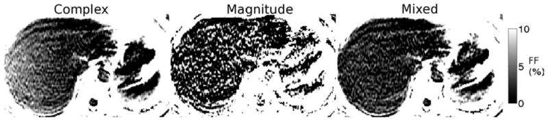
Results in patients from an acquisition with TEmin = 1.2 ms, ΔTE = 2.0 ms (i.e., outside the “blue hole” for magnitude fitting) are shown in Fig. 4. Because of phase errors present in the data, complex fitting results in severe bias in the FF estimates, particularly near the edge of the field of view along the readout direction (R/L). The apparent gradient in FF is due to phase errors and disappears when phase errors are corrected using either magnitude or mixed fitting. For datasets acquired using these TEs, both magnitude and mixed fitting are able to provide accurate FF estimates with good SNR. Figure 5 shows a comparison of FF estimates from 84 studies (42 patients) using this same echo time combination. Imaging results using complex, magnitude and mixed fitting are compared with single voxel spectroscopy (STEAM-MRS) FF estimates. In these exams, complex fitting results in an overestimation of FF of nearly 5%, particularly at low true FFs, due to phase errors in the data. Both magnitude and mixed fitting are able to overcome these phase errors.
FIG. 4.

Representative fat fraction maps from complex, magnitude and mixed fitting from a dataset with echo combination “C” outside the “blue hole” (good magnitude fitting SNR). The complex fitting FF presents significant error, particularly further from the center of the FOV along the frequency-encoding direction (R/L). For this subject, the MRS FF = 2.4%. The coregistered FFs were: complex: 5.8%, magnitude: 2.0%, mixed: 2.3%.
FIG. 5.

Fat fraction estimation results from the datasets with echo combination “C” outside the “blue hole” (good magnitude fitting SNR). Both magnitude and mixed fitting are able to remove the bias present in complex fitting (particularly at low fat fractions). The mixed fitting slope is not significantly different from 1 (P = 0.11), and the intercept is not significantly different from 0 (P = 0.16).
In vivo liver results from an acquisition with TEmin = 1.3 ms, ΔTE = 2.1 ms (i.e., inside the “blue hole” for magnitude fitting) are shown in Fig. 6. The complex fitting FF results contain positive bias. For this echo time combination, magnitude fitting results in unstable (extremely noisy) estimates and its results are not reliable. Mixed fitting is able to remove the bias while maintaining good SNR performance. Figure 7 shows a comparison of FF estimates from 20 studies (10 patients) obtained using this same echo time combination. Imaging results using complex and mixed fit-ting are compared with STEAM-MRS FF estimates. Mixed fitting effectively avoids the bias resulting from complex fitting. Magnitude fitting results are not included, since the results were highly unstable.
FIG. 6.
Representative fat fraction maps from complex, magnitude and mixed fitting from a dataset with echo combination “D” in the “blue hole” (poor magnitude fitting SNR). The complex fitting FF presents significant error, particularly further from the center of the FOV along the frequency-encoding direction (R/L). For this subject, the MRS FF = 1.3%. The coregistered FFs were: complex: 4.4%, magnitude: 4.9%, mixed: 1.1%. Magnitude results are unreliable due to high noise for this echo time combination.
FIG. 7.

Fat fraction estimation results on the datasets with echo combination “D” in the “blue hole” (poor magnitude fitting SNR). Magnitude fitting results were not included because these estimates were unstable for this echo combination. Complex fitting results in significant bias, particularly at low fat fractions. Mixed fitting is able to remove this bias. The mixed fitting slope is not significantly different from 1 (P = 0.37), and the intercept is not significantly different from 0 (P = 0.83).
DISCUSSION
We have demonstrated that the proposed mixed fitting method provides FF measurements in the presence of phase errors, with low bias and good SNR for wide choice of echo time combinations. This is particularly relevant for 1.5T single-shot acquisitions, where the echo spacing often leads to poor SNR performance in magnitude fitting. Additionally, by only discarding the phase of the first echo, mixed fitting avoids the ambiguity for FFs above or below 50%.
Yu et al. (23) recently proposed a hybrid magnitude/complex fitting method, where the estimates from complex and magnitude fitting are combined with different weights depending on the FF (for instance, hybrid estimates at low FFs will be nearly equal to magnitude fitting estimates, whereas at FFs near 50% they will be nearly equal to complex fitting estimates). Relative to this hybrid method, the proposed mixed fitting method has improved noise performance, particularly at low FFs and for echo time combinations near the “blue holes” (see Fig. 2).
Mixed fitting assumes a priori knowledge on which phase measurements are reliable and which are not. This method can be extended to more sophisticated phase behavior, as is the case in multi-shot acquisitions or acquisitions with nonuniformly spaced TEs. Additionally, the mixed fitting approach may be useful in other applications with different pulse sequences that can lead to phase errors, e.g., unspoiled sequences.
It must be noted that the advantages of mixed fitting (relative to magnitude fitting) vary with experimental conditions. For instance, acquisitions at 3T are more easily performed using two interleaved echo trains (“two-shot” acquisitions). The reason is that the fat-water chemical shift is doubled at 3T (relative to 1.5T), complicating the acquisition of favorable echo spacings to attain high NSA (29). In these two-shot acquisitions, typical echo time combinations do not fall into NSA “blue holes” for magnitude fitting and there is less need for a mixed fitting solution (although the NSA of mixed fitting will always be at least as high as that of magnitude fitting).
Mixed fitting can be applied to other signal models, such as dual- fat-water models (where separate decay rates are modeled for the water and fat signals). Phase errors in the data become even more problematic in dual- fitting (compared to single- ), where fitting for the fat at low FFs is very sensitive to noise and signal artifacts (including phase errors). In preliminary tests on patient data (not shown), dual- complex fitting in the presence of phase errors can result in large errors in the apparent fat , which in turn result in large errors in the estimated FFs. These errors can be avoided using dual- mixed fitting. Note that dual- fitting (either complex or mixed) results in significantly noisier FF estimates compared with single- fitting (17,18). Additionally, mixed fitting can also be applied to models with more than two distinct chemical species.
Alternatively to the proposed mixed fitting method, a calibration scan-based correction method could be included in the pulse sequence, similarly to those performed in EPI acquisitions. Such a method would be doable but require a modified acquisition, with additional calibrating readout lines. The proposed method has the advantage of allowing accurate fat quantification for a wide choice of TE combinations, without requiring additional calibration scans. It also allows correction of datasets that have already been acquired (where complex fitting may lead to bias and magnitude fitting may lead to low SNR).
The detailed cause of these phase errors is beyond the scope of this work. However, based on previous investigations, these phase errors likely result from gradient-induced eddy currents and possibly mechanical vibration (38–40). Regardless of the cause, the quantitative results (where mixed fitting largely removes the bias in FF estimation) indicate that, for typical acquisitions, phase information is reliable for echoes other than the first one.
CONCLUSIONS
Phase errors in the acquired signal can result in significant errors in FF estimation. Magnitude fitting (where all phase information is discarded) overcomes these phase errors but results in severe SNR losses, particularly for certain choices of echo time combinations. Through careful modeling of the acquired signal, the proposed mixed fitting method enables accurate fat quantification with good SNR performance, low bias and over a wide range of echo time combinations.
Acknowledgments
Grant sponsor: NIH; Grant numbers: R01 DK083380, R01 DK088925, RC1 EB010384; Grant sponsors: Coulter Foundation, GE Healthcare
The authors thank Gavin Hamilton for the STEAM-MRS pulse sequence.
References
- 1.Ratziu V, Charlotte F, Heurtier A, Gombert S, Giral P, Bruckert E, Grimaldi A, Capron F, Poynard T. Sampling variability of liver biopsy in nonalcoholic fatty liver disease. Gastroenterology. 2005;128:1898–1906. doi: 10.1053/j.gastro.2005.03.084. [DOI] [PubMed] [Google Scholar]
- 2.Hussain HK, Chenevert TL, Londy FJ, Gulani V, Swanson SD, McKenna BJ, Appelman HD, Adusumilli S, Greenson JK, Conjeevaram HS. Hepatic fat fraction: MR imaging for quantitative measurement and display–early experience. Radiology. 2005;237:1048–1055. doi: 10.1148/radiol.2373041639. [DOI] [PubMed] [Google Scholar]
- 3.Kim H, Taksali SE, Dufour S, Befroy D, Goodman TR, Petersen KF, Shulman GI, Caprio S, Constable RT. Comparative MR study of hepatic fat quantification using single-voxel proton spectroscopy, two-point dixon and three-point IDEAL. Magn Reson Med. 2008;59:521–527. doi: 10.1002/mrm.21561. [DOI] [PMC free article] [PubMed] [Google Scholar]
- 4.Reeder SB, Robson PM, Yu H, Shimakawa A, Hines CDG, McKenzie CA, Brittain JH. Quantification of hepatic steatosis with MRI: the effects of accurate fat spectral modeling. J Magn Reson Imaging. 2009;29:1332–1339. doi: 10.1002/jmri.21751. [DOI] [PMC free article] [PubMed] [Google Scholar]
- 5.Yokoo T, Bydder M, Hamilton G, Middleton MS, Gamst AC, Wolfson T, Hassanein T, Patton HM, Lavine JE, Schwimmer JB, Sirlin CB. Nonalcoholic fatty liver disease: diagnostic and fat-grading accuracy of low-flip-angle multiecho gradient-recalled-echo MR imaging at 1.5 T. Radiology. 2009;251:67–76. doi: 10.1148/radiol.2511080666. [DOI] [PMC free article] [PubMed] [Google Scholar]
- 6.Glover GH, Schneider E. Three-point Dixon technique for true water/fat decomposition with B0 inhomogeneity correction. Magn Reson Med. 1991;18:371–383. doi: 10.1002/mrm.1910180211. [DOI] [PubMed] [Google Scholar]
- 7.Xiang QS, An L. Water-fat imaging with direct phase encoding. J Magn Reson Imaging. 1997;7:1002–1015. doi: 10.1002/jmri.1880070612. [DOI] [PubMed] [Google Scholar]
- 8.An L, Xiang QS. Chemical shift imaging with spectrum modeling. Magn Reson Med. 2001;46:126–130. doi: 10.1002/mrm.1167. [DOI] [PubMed] [Google Scholar]
- 9.Ma J. Breath-hold water and fat imaging using a dual-echo two-point Dixon technique with an efficient and robust phase-correction algorithm. Magn Reson Med. 2004;52:415–419. doi: 10.1002/mrm.20146. [DOI] [PubMed] [Google Scholar]
- 10.Reeder SB, Wen Z, Yu H, Pineda AR, Gold GE, Markl M, Pelc NJ. Multicoil Dixon chemical species separation with an iterative least squares estimation method. Magn Reson Med. 2004;51:35–45. doi: 10.1002/mrm.10675. [DOI] [PubMed] [Google Scholar]
- 11.Yu H, Reeder SB, Shimakawa A, Brittain JH, Pelc NJ. Field map estimation with a region growing scheme for iterative 3-point water-fat decomposition. Magn Reson Med. 2005;54:1032–1039. doi: 10.1002/mrm.20654. [DOI] [PubMed] [Google Scholar]
- 12.Lu W, Hargreaves BA. Multiresolution field map estimation using golden section search for water-fat separation. Magn Reson Med. 2008;60:236–244. doi: 10.1002/mrm.21544. [DOI] [PubMed] [Google Scholar]
- 13.Hernando D, Kellman P, Haldar JP, Liang ZP. Robust water/fat separation in the presence of large field inhomogeneities using a graph cut algorithm. Magn Reson Med. 2010;63:79–90. doi: 10.1002/mrm.22177. [DOI] [PMC free article] [PubMed] [Google Scholar]
- 14.Liu CY, McKenzie CA, Yu H, Brittain JH, Reeder SB. Fat quantification with IDEAL gradient echo imaging: Correction of bias from T1 and noise. Magn Reson Med. 2007;58:354–364. doi: 10.1002/mrm.21301. [DOI] [PubMed] [Google Scholar]
- 15.Yu H, McKenzie CA, Shimakawa A, Vu AT, Brau ACS, Beatty PJ, Pineda AR, Brittain JH, Reeder SB. Multiecho reconstruction for simultaneous water-fat decomposition and T2* estimation. J Magn Reson Imaging. 2007;26:1153–1161. doi: 10.1002/jmri.21090. [DOI] [PubMed] [Google Scholar]
- 16.Bydder M, Yokoo T, Hamilton G, Middleton MS, Chavez AD, Schwimmer JB, Lavine JE, Sirlin CB. Relaxation effects in the quantification of fat using gradient echo imaging. Magn Reson Imaging. 2008;26:347–359. doi: 10.1016/j.mri.2007.08.012. [DOI] [PMC free article] [PubMed] [Google Scholar]
- 17.Chebrolu VV, Hines CD, Yu H, Pineda AR, Shimakawa A, McKenzie C, Brittain JH, Reeder SB. Independent estimation of T2* for water and fat for improved accuracy of fat quantification. Proceedings of the 17th Annual Meeting of ISMRM; Honolulu, Hawaii, USA. 2009. p. 2847. [Google Scholar]
- 18.Hernando D, Liang ZP, Kellman P. Chemical shift-based water/fat separation: a comparison of signal models. Magn Reson Med. 2010;64:811–822. doi: 10.1002/mrm.22455. [DOI] [PMC free article] [PubMed] [Google Scholar]
- 19.Yu H, Shimakawa A, McKenzie CA, Brodsky EK, Brittain JH, Reeder SB. Multiecho water-fat separation and simultaneous R2* estimation with multifrequency fat spectrum modeling. Magn Reson Med. 2008;60:1122–1134. doi: 10.1002/mrm.21737. [DOI] [PMC free article] [PubMed] [Google Scholar]
- 20.Brodsky EK, Holmes JH, Yu H, Reeder SB. Generalized k-space decomposition with chemical shift correction for non-cartesian water-fat imaging. Magn Reson Med. 2008;59:1151–1164. doi: 10.1002/mrm.21580. [DOI] [PubMed] [Google Scholar]
- 21.Yu H, Shimakawa A, Reeder SB, McKenzie CA, Brittain JH. Magnitude fitting following phase sensitive water-fat separation to remove effects of phase errors. Proceedings of the 17th Annual Meeting of ISMRM; Honolulu, Hawaii, USA. 2009. p. 461. [Google Scholar]
- 22.Szczepaniak LS, Nurenberg P, Leonard D, Browning JD, Reingold JS, Grundy S, Hobbs HH, Dobbins RL. Magnetic resonance spectroscopy to measure hepatic triglyceride content: prevalence of hepatic steatosis in the general population. Am J Physiol Endocrinol Metab. 2005;288:E462–468. doi: 10.1152/ajpendo.00064.2004. [DOI] [PubMed] [Google Scholar]
- 23.Yu H, Shimakawa A, McKenzie CA, Hines CDG, McKenzie CA, Hamilton G, Sirlin CB, Brittain JH, Reeder SB. Combination of complex-based and magnitude-based multiecho water-fat separation for accurate quantification of fat-fraction. Magn Reson Med. 2011 doi: 10.1002/mrm.22840. [Epub ahead of print] [DOI] [PMC free article] [PubMed] [Google Scholar]
- 24.Meisamy S, Hines CD, Hamilton G, Sirlin CB, McKenzie CA, Yu H, Brittain JH, Reeder SB. Quantification of hepatic steatosis with T1-independent, T2*-corrected MR imaging with spectral modeling of fat: blinded comparison with MR spectroscopy. Radiology. 2011;258:767–775. doi: 10.1148/radiol.10100708. [DOI] [PMC free article] [PubMed] [Google Scholar]
- 25.Yu H, Shimakawa A, Hernando D, Hines CDG, McKenzie CA, Reeder SB, Brittain JH. Noise Performance of Magnitude-Based Water-Fat Separation is Sensitive to the Echo Times. Proceedings of the 19th annual meeting of ISMRM; Montreal, Canada. 2001. p. 2715. [Google Scholar]
- 26.Middleton MS, Hamilton G, Bydder M, Sirlin CB. How Much Fat is Under the Water Peak in Liver Fat MR Spectroscopy?. Proceedings of the 17th annual meeting of ISMRM; Honolulu, Hawaii. 2009. p. 4331. [Google Scholar]
- 27.Hamilton G, Yokoo T, Bydder M, Cruite I, Schroeder ME, Sirlin CB, Middleton MS. In vivo characterization of the liver fat 1H MR spectrum. NMR Biomed. 2011 doi: 10.1002/nbm.1622. [Epub ahead of print] [DOI] [PMC free article] [PubMed] [Google Scholar]
- 28.Scharf LL, McWhorter LT. Geometry of the Cramér-Rao Bound. Proceedings of the IEEE Sixth SP Workshop on Statistical Signal and Array Processing; Victoria, BC, Canada. 1992. pp. 5–8. [Google Scholar]
- 29.Pineda A, Reeder S, Wen Z, Pelc NJ. Cramér-Rao bounds for three-point decomposition of water and fat. Magn Reson Med. 2005;54:625–635. doi: 10.1002/mrm.20623. [DOI] [PubMed] [Google Scholar]
- 30.Chebrolu VV, Yu H, Pineda AR, McKenzie CA, Brittain JH, Reeder SB. Noise analysis for 3-point chemical shift-based water-fat separation with spectral modeling of fat. J Magn Reson Imaging. 2010;32:493–500. doi: 10.1002/jmri.22220. [DOI] [PMC free article] [PubMed] [Google Scholar]
- 31.Karlsen OT, Verhagen R, Bovée WM. Parameter estimation from Rician-distributed data sets using a maximum likelihood estimator: application to T1 and perfusion measurements. Magn Reson Med. 1999;41:614–623. doi: 10.1002/(sici)1522-2594(199903)41:3<614::aid-mrm26>3.0.co;2-1. [DOI] [PubMed] [Google Scholar]
- 32.Walsh DO, Gmitro AF, Marcellin MW. Adaptive reconstruction of phased array MR imagery. Magn Reson Med. 2000;43:682–690. doi: 10.1002/(sici)1522-2594(200005)43:5<682::aid-mrm10>3.0.co;2-g. [DOI] [PubMed] [Google Scholar]
- 33.Hines CD, Yu H, Shimakawa A, McKenzie CA, Brittain JH, Reeder SB. T1 independent, T2* corrected MRI with accurate spectral modeling for quantification of fat: validation in a fat-water-SPIO phantom. J Magn Reson Imaging. 2009;30:1215–1222. doi: 10.1002/jmri.21957. [DOI] [PMC free article] [PubMed] [Google Scholar]
- 34.Hines CDG, Frydrychowicz AP, Tudorascu DL, Hamilton G, Vigen KK, Yu H, McKenzie CA, Sirlin CB, Brittain JH, Reeder SB. T1 Independent, T2* Corrected Chemical Shift Based Fat-Water Separation with Accurate Spectral Modeling is an Accurate and Precise Measure of Liver Fat. Proceedings of the 18th Annual Meeting of ISMRM; Honolulu, Haway, USA. 2010. p. 263. [Google Scholar]
- 35.Hamilton G, Middleton MS, Bydder M, Yokoo T, Schwimmer JB, Kono Y, Patton HM, Lavine JE, Sirlin CB. Effect of PRESS and STEAM sequences on magnetic resonance spectroscopic liver fat quantification. J Magn Reson Imaging. 2009;30:145–152. doi: 10.1002/jmri.21809. [DOI] [PMC free article] [PubMed] [Google Scholar]
- 36.de Bazelaire CM, Duhamel GD, Rofsky NM, Alsop DC. MR imaging relaxation times of abdominal and pelvic tissues measured in vivo at 3. 0 T: preliminary results. Radiology. 2004;230:652–659. doi: 10.1148/radiol.2303021331. [DOI] [PubMed] [Google Scholar]
- 37.Hines CDG, Yokoo T, Bydder M, Sirlin CB, Reeder SB. Optimization of Flip Angle to Allow Tradeoffs in T1 Bias and SNR Performance for Fat Quantification. Proceedings of the 18th annual meeting of ISMRM; Honolulu, Hawaii, USA. 2010. p. 2927. [Google Scholar]
- 38.Ryner LN, Stroman P, Wessel T, Hoult DI, Saunders JK. Effect of Oscillatory Eddy Currents on MR Spectroscopy. Proceedings of the 6th Annual Meeting of ISMRM; Sidney, Australia. 1998. p. 1903. [Google Scholar]
- 39.Bernstein MA, King KF, Zhou XJ. Handbook of MRI pulse sequences. Burlington: Academic Press; 2004. [Google Scholar]
- 40.Nixona TW, McIntyrea S, Rothmana DL, de Graaf RA. Compensation of gradient-induced magnetic field perturbations. J Magn Reson. 2008;192:209–217. doi: 10.1016/j.jmr.2008.02.016. [DOI] [PMC free article] [PubMed] [Google Scholar]