


Abstract
Typical approaches for predicting transcription factor binding sites (TFBSs) involve use of a position-specific weight matrix (PWM) to statistically characterize the sequences of the known sites. Recently, an alternative physicochemical approach, called SiteSleuth, was proposed. In this approach, a linear support vector machine (SVM) classifier is trained to distinguish TFBSs from background sequences based on local chemical and structural features of DNA. SiteSleuth appears to generally perform better than PWM-based methods. Here, we improve the SiteSleuth approach by considering both new physicochemical features and algorithmic modifications. New features are derived from Gibbs energies of amino acid–DNA interactions and hydroxyl radical cleavage profiles of DNA. Algorithmic modifications consist of inclusion of a feature selection step, use of a nonlinear kernel in the SVM classifier, and use of a consensus-based post-processing step for predictions. We also considered SVM classification based on letter features alone to distinguish performance gains from use of SVM-based models versus use of physicochemical features. The accuracy of each of the variant methods considered was assessed by cross validation using data available in the RegulonDB database for 54 Escherichia coli TFs, as well as by experimental validation using published ChIP-chip data available for Fis and Lrp.
INTRODUCTION
Transcription factors (TFs) are key molecular components of gene regulatory networks that modulate gene expression by binding to DNA and affecting the ability of RNA polymerase to transcribe genes. Thus, methods for identifying TF binding sites (TFBSs) in DNA can provide important insights into cell biology and may in the future help to enable exquisite manipulation of cellular behavior through synthetic and systems biology approaches (1,2).
A large number of binding sites for diverse TFs have been characterized through targeted low-throughput experimental approaches. Additionally, several high-throughput methods, such as chromatin immunoprecipitation coupled to sequencing (ChIP-seq) and protein binding microarray (PBM) assays, are now available for large-volume detection of binding sites (3–5). TFBSs discovered through both low- and high-throughput approaches are documented in databases such as RegulonDB (6) and JASPAR (7). These methods and the increasing catalog of TFBSs are providing new insights into the general nature of TF–DNA interactions and promise to elucidate how TF binding specificity is achieved (8).
Experimental approaches for characterizing TFBSs are complemented by computational approaches, which can provide a level of detail inaccessible experimentally. For example, ChIP-seq binding sites are limited to a precision of a couple hundred base-pairs (bp) (9), which is much longer than actual TFBSs. Computational methods typically aim to model sets of TFBSs as (sequence) motifs (5,10), built on the basis of a set of training data. A motif model can be used to summarize data, to more precisely localize a binding site within a region of DNA known to associate with a TF, to design experiments, or to predict the effect of a mutation on a known TFBS. It can also provide insights into the features of DNA sequences important for TF–DNA recognition.
A common approach to motif representation or motif modeling involves the construction of a position-specific weight matrix (PWM) or a consensus sequence (10). There are many methods, as well as software tools, for modeling TFBSs in terms of PWMs (11–17), as well as more advanced techniques that consider dependencies between nucleotides in different positions (18), but the vast majority are based on the assumption that letter representations of DNA sequences suitably capture the physicochemical properties of DNA (and proteins) that govern the specificity of protein–DNA interactions. However, the general validity of this assumption is questionable (19).
The three-dimensional (3D) structure of DNA is sequence dependent (20,21), and shape readout is an important mode of recognition used by a large class of TFs (22–25). However, letter sequence similarity does not guarantee structure similarity and vice versa: DNA sequences can diverge at the level of letter representation but share a similar structure, and conversely, DNA sequences can differ in only one or two bases but have distinct local structures (20,22,26). There is strong evidence that TFs that recognize one particular sequence can also recognize different sequences if the sequences have similar structural properties, and more generally that some TFs interact with multiple classes of DNA sequences at the level of letter representation (21–24,27–29). Interestingly, it was recently reported that Hoogsteen base pairs, which are characterized by a pattern of hydrogen bonding that differs from that of Watson–Crick base pairs, are present in free DNA in equilibrium with Watson–Crick base pairs (30). These discoveries imply that TF-DNA binding specificity is extremely unlikely to be described by a simple linear code (31). The simple reason is that, with this newfound understanding of the plasticity of DNA structure, a letter code for a DNA sequence can no longer be taken to have an unambiguous structural interpretation.
Moving beyond analysis of letter codes, researchers have made a number of attempts to use structural data to predict TFBSs (32–42). Some approaches focus on shape readout, although this is relevant only for some TFs. A second important mode of recognition is base readout (22), which involves direct contacts between nucleotides and amino acid residues. In other words, some TFs scan the chemical signatures of DNA sequences, not their shapes alone. Methods that rely on atomic structures of protein–DNA complexes can address these cases but are computationally more expensive and depend strongly on the quality of experimental structures (35). In some cases homology structure predictions can provide some of these details, but these calculations still require a degree of expertize in structural modeling.
Although promising results have been obtained by all-atom approaches in some cases, there is a need for methods that consider details at an intermediate resolution, between the fine resolution of atomic characterization of macromolecular complexes and the coarse resolution of letter representations of DNA. In particular, we believe that a method requiring only the sequences of known binding sites (i.e. the same inputs as standard PWM approaches) but using physical properties of DNA to construct a TFBS model could begin to approach the accuracy of structure-based models while retaining the accessibility of the usual PWM models.
Recently, we reported a motif modeling approach based on local structural and chemical features of DNA (26). This approach, which we called SiteSleuth, maps DNA sequences to physicochemcial features and uses a support vector machine (SVM) classifier that discriminates between known TFBSs and genome background sequences. The features considered include structural features, which characterize the local conformation of a DNA sequence, and chemical features, which characterize the thermodynamics of interactions between small functional group probes and a DNA sequence. The SiteSleuth method typically performs better than commonly used PWM-based methods (26).
Here, we report an improvement of the SiteSleuth method obtained by considering both new physicochemical features and algorithmic modifications (i.e. variations on the machine learning approach). We examine each improvement by implementing them one by one into distinct motif models, and by comparing to a standard PWM-based algorithm. In all, we compare six methods. To evaluate the different motif modeling approaches, we focused on 54 TFs in Escherichia coli and their binding sites documented in RegulonDB (6), measuring the accuracy of each model through cross validation. We also used ChIP-chip binding data available for the E. coli TFs Fis and Lrp (43,44).
MATERIALS AND METHODS
Our physicochemical motif modeling approach is based on two essential ingredients: physicochemical features of DNA, and supervised machine learning, in particular the use of SVMs to discriminate known TFBSs from background genome sequences. In this section, we first describe calculation of the various features used in our motif models and show how DNA sequences are mapped to those features. We consider two main classes of physicochemical features: structural features, which characterize the conformational rigidity and steric properties of DNA, and chemical features, which characterize the electrostatic profile around DNA. We also introduce letter features, which makes the information used in training an SVM the same as that used in standard PWM-based approaches. We distinguish the new models using physicochemical features or letter features by including PMM or LMM (for physical motif model or letter-based motif model), respectively, in their name. Second, we describe the details of the training and predicting aspects of the machine learning approach that we use, which is based on SVMs. We discuss optimization of SVM parameters through grid search, the differences between the linear and radial basis function (RBF) SVM kernels, improvements in the training step through feature selection, and improvements in the prediction step through consensus-based post-processing of the positive predictions. Finally, we discuss the sources of data used for training and testing.
Definition and use of feature sets
Structural features
Our structural features are based on free DNA properties. Because structural correlations have been observed between free and bound TFBSs (45), we expect that these properties will be relevant for TFBSs prediction. First, parameters describing the geometry of base pairs and bp steps were derived from duplex structures of short DNA sequences (all possible 3- and 4-mers embedded between flanking GC dinucleotides), which were found via molecular dynamics (MD) simulations as described previously (26). Briefly, for each duplex, the initial structure was taken to be the standard Watson and Crick structure for B-DNA. The NAMD program (46) and the CHARMM27 force field (47–50) were then used to produce an equilibrium average structure. For the middle base pair in each of the 64 possible 3-mers, we used normal mode analysis of the corresponding average structure to calculate six base-pairing parameters: shear, stretch, stagger, buckle, propeller and opening. Similarly, for the middle 2 bp in each of the 256 possible 4-mers, we used normal mode analysis of the corresponding average structure to calculate 6 bp step parameters: shift, tilt, slide, roll, rise and twist. Features derived from simulated structures have been shown to correlate with features derived from experimentally determined structures (26).
In addition to the geometric parameters described above, which were considered in earlier work (26), we also considered a structural profile defined on the basis of hydroxyl radical cleavage of DNA (20,53,54). This profile has been shown to correlate with various aspects of DNA structure (54), as the global structure of a DNA sequence imposes localized steric constraints on hydroxyl radical cleavage propensity (20). The ORChID (OH Radical Cleavage Intensity Database) resource provides tools for predicting the hydroxyl radical cleavage profile of a given DNA sequence (53). The profile is calculated by sliding a 4 bp window across the sequence and averaging over a database of experimentally measured cleavage profiles to generate a cleavage propensity at each nucleotide. Within the ORChID tool, the cleavage propensity at each position is completely determined by the three flanking nucleotides on each side of a central nucleotide, so our hydroxyl radical cleavage feature list consists of the calculated structural profiles for all possible 7-mers (47 = 16 384). Each of these 7-mers is associated with two structural features: the cleavage propensities of the central nucleotides of the forward and reverse strands.
Chemical features
Structural features characterize the conformation of free DNA. Here, we introduce chemical features to characterize the electrostatic profile around DNA, which can be expected to influence site-specific protein–DNA interactions. In earlier work, 31 small functional groups were used as probes, and thermodynamic parameters were calculated to characterize an array of probe and DNA configurations (26). Here, we consider the 20 common amino acids as probes of the DNA electrostatic profile. For a given probe, different spatial configurations of the probe and a DNA duplex are generated. Thermodynamic parameters are calculated for each configuration and an average over the configurations is determined. Features based on functional group probes were calculated as described previously (26). For amino acid probes, a similar approach is followed, except sampling of configurations is now more extensive because amino acids are relatively large, and as a result, thermodynamic parameters are more sensitive to configurational aspects of probe–DNA interaction. These features, which are introduced in this study, are determined as described below.
Initial structures of amino acids capped by an acetyl group at the N-terminus and an N-methylamide group at the C-terminus were obtained using CHARMM34b1 (55). These structures were paired with equilibrated, average structures of DNA 3-mers (with flanking GC dinucleotides), calculated as described above. For each of the 20 × 64 amino acid-DNA duplex pairs, we considered the following spatial configurations of the two molecules. As illustrated in Figure 1, for each of the two central nucleotides in the DNA duplex, we considered a 6 × 6 × 3 grid filling a rectangular box. For each grid, the α-carbon of the amino acid probe was placed at each of the 108 grid points. The initial orientation of the amino acid was arbitrary but consistent across grid points. At each grid point, we considered 81 distinct whole-molecule rotations. Each of these rotations was a composition of a rotation of angle θ ∈ [−π/2, −7π/18, −5π/18, … , π/2] around the x-axis and a rotation of angle ϕ ∈ [−π, −8π/9, −7π/9, … , π] around the z-axis (9 rotations each). At each grid point, we also considered fifteen side-chain rotamers for all amino acid probes except alanine, glycine and proline. Rotamers of an amino acid were generated by rotating the side chain around the bond between the α- and β-carbons (χ1 dihedral; additional rotations around χ2, χ3 etc. were not considered). The angles of rotations were integer multiples of 2π/15 (see Figure S1 of the Supplementary Materials for more details on how the angle increments were chosen). Thus, for each side of a DNA duplex, we considered a total of 2 256 984 probe-duplex configurations (108 × 81 × (17 × 15 + 3)).
Figure 1.

Schematic of amino acid–DNA interaction. The DNA structure for sequence CAG (and two flanking GC pairs on either end) is superimposed with 108 grid points around the center adenosine nucleotide arranged in a 6 × 6 × 3 grid and a sample isoleucine structure; the three sub-grids in the DNA minor groove, major groove and outside the DNA are colored orange, red and purple, respectively. G is colored green, C blue, A yellow and T red. In the calculations, the α-C of the amino acid is centered at each grid point and rotations and energy calculations are performed as described in Materials and Methods. The grid is defined by six bounding planes: the bounding planes above and below the grid are centered halfway between the central A and the adjacent nucleotides C and G above and below, respectively, and are parallel to each other as well as to the plane of the rings in adenine. The bounding plane on the left is centered between the A and T base-pairing nucleotides and is perpendicular to the previously defined planes. The bounding plane on the right is placed 20Å from the plane on the left (and parallel to it). The bounding planes in and out of the page are perpendicular to all previously defined planes and 10Å in or out from the center of the adenine ring. Thus the volume of the grid is 20 × 20 × D Å3, where D is the distance between adjacent nucleotides, typically about 3.5 Å. This figure was created using VMD (51,52).
For each amino acid-DNA duplex pair (Figure 1), we estimated the Gibbs free energy at each grid point p using the expression Gp = −kBTlnZp, where kB is the Boltzmann constant, T is the absolute temperature, which we took to be 298 K, and Zp is the partition function ∑q exp(−Epq/kBT). In the partition function, q is an index for the elements of the set of all whole-molecule rotations and all side-chain rotations (if any), and Epq is the total energy given by NAMD and the CHARMM27 force field with the probe at grid point p in orientation q. The change in Gibbs free energy caused by interaction between the probe at a grid point and the DNA duplex, ΔGp, was found by subtracting the Gibbs free energy obtained when the probe and DNA duplex were separated by a large distance, G. In other words, ΔGp ≡ Gp − G.
To define chemical features, we first split up the grid into three sub-grids: two 3 × 3 × 3 grids in the minor and major grooves of the DNA and a 6 × 3 × 3 grid outside the DNA (orange dots, red dots and purple dots in Figure 1, respectively). For each sub-grid, we computed the average (over all favorable grid points with ΔG < 0), ΔGavg, and minimum, Δ Gmin. This procedure resulted in 120 values for each side of a DNA duplex (minimum and average ΔG for each of three sub-grids and 20 amino acids). Many amino acids may have similar interaction profiles with the various 3-mers, so many of these 120 dimensions are highly correlated across different DNA sequences. To eliminate correlated feature dimensions while retaining the essential information about the electrostatic profile encapsulated in the chemical features, we used principal component analysis (PCA) to generate orthogonal vectors that capture the variability of the original feature set; we normalized each of the 120 dimensions (across all 64 possible 3-mers) to have mean 0 and standard deviation 1 prior to performing PCA. We chose the top 20 principal components as an abbreviated feature list, which captured 90.5% of the variance. The final feature list was obtained by concatenating the features for each side of the DNA duplex. Thus, the chemical features consist of 40 values (20 for each strand) associated with the center nucleotide of each DNA 3-mer.
Letter features
The structural and chemical features discussed above are one facet of SVM-PMM and SiteSleuth that distinguishes these methods from other TFBSs prediction algorithms, such as PWM-based methods and other methods based on letter representations of DNA sequences (11–14). The other main difference is the use of an SVM classifier. Because it was previously found that SiteSleuth outperforms other TFBSs prediction algorithms (26), we wanted to measure how much of this improvement can be attributed to the use of SVM-based classification versus the use of physicochemical features. To this end, we created an LMM that uses features designed to encode letter sequences: orthonormal 4D vectors (1,0,0,0), (0,1,0,0), (0,0,1,0) and (0,0,0,1) are designated as feature vectors of the single nucleotides A, C, G and T, respectively. Using letter features, we can independently assess the effects of using SVM-based classification and physicochemical features in PMMs. We will use ‘SVM-LMM’ to refer to TFBSs models that take letter features as input for training.
Mapping DNA sequences to feature vectors
To associate DNA sequences of known or potential TFBSs with positions in a space of features, in which negative and positive examples can be separated using the SVM approach to classification, we map each sequence to a feature vector of real numbers. Each scalar component of a feature vector corresponds to a letter, structural or chemical feature. Although it is time consuming to calculate the structural and chemical features of (short) DNA sequences, the mapping procedure described below allows us to pre-calculate and store sets of features and then to efficiently determine the physicochemical features of any new given DNA sequence.
The procedure for mapping a given DNA sequence to a feature vector is illustrated in Figure 2. Before starting this procedure, we select a known or potential binding site sequence (Figure 2A), we add flanking nucleotides at each end (lower case) in accordance with the genome sequence, and we identify the sets of pre-calculated features for short sequences that will be considered (Figure 2B). In SVM-PMM, four feature sets are considered: (i) amino acid–DNA chemical features (αi); (ii) structural base-pairing features (βi); (iii) structural bp step features (γi); and (iv) structural hydroxyl radical cleavage features (δi). Within a feature set, K features are associated with each of the possible DNA sequences of length N. Set (i) associates 20 features with each of the possible 3-mers (i.e. αi ∈  20, i = 1, … , 64): Set (ii) associates six features with each of the possible 3-mers: Set (iii) associates six features with each of the possible 4-mers: and Set (iv) associates two features with each of the possible 7-mers. In the case of letter features (not considered in Figure 2), four features (three 0's and one 1) are associated with each of the four 1-mers.
Figure 2.

Schematic of feature mapping procedure. For illustration, we demonstrate the mapping with the features used in SVM-PMM. (A) For a given sequence, we include three flanking sequences (lower case letters) on either side. (B) N-mers of length 3, 4 and 7 are slid across the sequence (the first 3-mer subsequence is indicated in panel (A)) and the resulting subsequences are mapped to chemical features α, structural bp features β, structural bp step features γ and hydroxyl radical cleavage features δ. (C) Those features are concatenated into a feature vector x for the sequence. The feature vector for this 10-mer will have 334 dimensions (6 + 20 for each of 10 3-mers, 2 for each of 10 7-mers and 6 for each of 9 4-mers).
To map a given DNA sequence to features, we start with the first nucleotide of the sequence proper (e.g. the first capital letter in Figure 2A). For each feature set of interest, we consider the appropriate length N-mer sliding window across the sequence, illustrated in Figure 2B. Thus, for Set (i) or (ii), for which N = 3, we consider the first nucleotide and its closest neighbors. The features associated with this N-mer are then concatenated to the feature vector for the sequence, as shown in Figure 2C. The example of Figure 2 is specific to SVM-PMM. The feature sets considered depend on the motif model under consideration, and motif models can incorporate different feature sets.
For a given set of sequences to be used in SVM training, we linearly scale each feature associated with these sequences such that the numerical values associated with a given feature across all sequences lie between −1 and 1. The purpose of this normalization step is to avoid differences in magnitude between feature dimensions overwhelming the differences within a feature dimension (56). To scale the features, once all training sequences are mapped to feature vectors, we examine xi,j (i over all sequences, j over all features) and determine Mj ≡ maxj(|xi,j|). We use xi,j/Mj as the components of feature vectors in SVM training. The values of Mj are saved and used to normalize components of feature vectors of test sequences.
Algorithmic details
Machine learning algorithm
Using LIBSVM (56), we train SVM classifiers to discriminate features of TFBSs from features of background genome sequences. The process is described below.
We are given m feature vectors {x1, … , xm}, where xi ∈ n and n is the number of features captured in each vector (recall that each feature corresponds to a single scalar quantity.) We are also given the corresponding m classification values {y1, … , ym}, where yi ∈ {−1, 1}. The feature vector xi is mapped to a higher dimensional space through a function ϕ, the form of which depends on the form of a kernel function. The kernel function k(zi, zj) = ϕ(zi)·ϕ(zj) defines a similarity measure between two points zi and zj. For a linear SVM,
| (1) |
which reflects use of a hyperplane to separate positive and negative examples. The RBF kernel is
| (2) |
where γ is a constant. Because positive training examples are often tightly clustered in feature space, whereas negative training examples tend to be more broadly distributed, the RBF kernel often gives more accurate results. However, training an SVM classifier with an RBF kernel is significantly more computationally expensive (56). Below, we use ‘SVM’ in the name of a method to denote use of a linear kernel, and we use ‘SVMR’ in the name of a method to denote use of an RBF kernel.
In training an SVM, we find a surface with weight vector w and offset d that separates the positive examples (i.e. the examples for which yi = 1) from the negative examples (i.e. the examples for which yi = − 1). This task is accomplished by solving the minimization problem
| (3) |
subject to the constraints
| (4) |
The adjustable parameters ξi (i ∈ [1, … , m]) are slack variables that are introduced to account for the fact that it is generally not possible to perfectly separate the training data. The C+ and C− parameters, which are called penalty parameters, are taken to have fixed values. The minimization problem is solved using quadratic programming techniques. The solution can be expressed as
| (5) |
where each αi is a Lagrange multiplier. The separating surface can be represented as
| (6) |
for feature vector x. Thus, given values for C+, C− and γ (if the RBF kernel is being used), the other SVM parameters (w, d and ξi for i = 1, … , m) are uniquely determined by the solution of the minimization problem described above.
The penalty parameters C+ and C− are introduced to balance the influences of positive and negative training data, which is important because we always have available many more negative examples than positive examples. Each of the C+, C− and γ (if the RBF kernel is being used) parameters affect the accuracy of a classifier and should be optimized for best results. Optimization of these parameters is performed as follows.
For an SVM with a linear kernel, we optimize C+ and C−. For an SVM with an RBF kernel, we set C+ = C− = C and optimize C and γ. In both cases, optimization is performed through a 2D grid search. In this search, the optimality of a grid point is assessed using a cross-validation procedure, which is described below. This approach to SVM parameter optimization is an adaptation of a method recommended in the LIBSVM guide (56). The search starts out over a coarse grid of points: C+, C− = {2−5, 2−3, … , 211} (in the case of a linear kernel), or C = {2−5, 2−3, … , 215} and γ = {2−15, 2−13, … , 25} (in the case of a radial kernel). The optimization is refined over two progressively finer grids in smaller increments around the best grid point from the previous grid (as assessed by the cross-validation procedure). For example, consider a linear kernel. If (C+, C−) = (25, 2−1) is the optimal result from the first grid search, the second grid search would be over C+ = {23, 24, 25, 26, 27} and C− = {2−3, 2−2, 2−1, 20, 21}. If (C+, C−) = (24, 20) is the optimal result from the second grid search, the third grid search would be over C+ = {23, 23.5, 24, 24.5, 25} and C− = {2−1, 2 − 0.5, 20, 20.5, 21}. Refinement stops after the third grid search.
Each grid point defines a pair of parameters. For each pair, we perform 3-fold cross-validation: the available training data are randomly split into three sets (as equal in size as possible) and each set is used to assess the prediction accuracy of an SVM classifier trained, as described above, on the other two sets. The accuracy of the classifier is quantified by the F-measure:
| (7) |
where p and r are precision and recall, respectively. These quantities are defined as
| (8) |
where TP, FP and FN are counts of true positives, false positives and false negatives from the cross-validation procedure.
Once optimal values for C+ and C− (or C and γ) are obtained through the process described above, these parameter values and all available training data are used to determine the remaining SVM parameters by solving the minimization problem described above. The optimal F-measure obtained after the third grid search (but before final determination of w, d and ξk) is taken to represent the accuracy of an SVM classifier. Once all SVM parameters are determined, an SVM classifier can be used for prediction: a test sequence is mapped to a feature vector z and w · ϕ(z) + d is evaluated (left-hand side of Equation (6)). If this value is positive (i.e. z is on the same side of the separating surface as the positive examples), the sequence is considered to be a binding site.
Feature selection
We evaluated a simple feature selection step to reduce the dimensionality of feature vectors, which results in decreased computation time and improved accuracy. Feature selection is done separately for each TF, with the aim of selecting the subset of features that most aptly describes DNA binding for that TF. Our feature selection step is performed prior to cross-validation and training of the SVM, so it depends only on the training data and the feature set used. The procedure is illustrated schematically in Figure S2A of the Supplementary Materials.
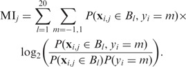
First, we compute the mutual information MIj (j = 1, … , n) between the j-th dimension of the training data, xi,j, and the training classifications yi; note that as j indexes the entire feature vector, it covers both the length of the binding site and all the features for each nucleotide of the binding site. Mutual information measures the dependence between two variables based on their probability distributions: a large value indicates greater dependence. Finding the distribution of yi is straightforward, as it takes only the values −1 and 1. After normalization, xi,j is a continuous variable between −1 and 1. We approximate its distribution by a discrete histogram with 20 bins of width of 0.1, which we denote as Bl = [−1 + (l − 1)/10, −1 + l/10), for l = 1, … , 20. The quantity MIj is then computed as
 |
(9) |
where P(xi,j ∈ Bl) and P(yi = m) are the marginal distributions of xi,j and yi (i.e. distributions computed over the training data, indexed by i) and P(xi,j ∈ Bl, yi = m) is the joint distribution.
After MIj has been computed for each feature dimension, we select the minimal subset of feature dimensions such that at least 90% of the total mutual information is retained. In other words, we ‘turn on’ dimensions one at a time, starting with the dimension with the largest MIj first, until the sum of all the ‘on’ MIj is at least 90% of the total (the sum over all j). The list of ‘on’ dimensions is determined from the training data and saved so that the same features are retained in the test data. We will indicate the use of the feature selection step in a method by adding ‘FS’ to its name. Figures S2B and C of the Supplementary Materials give statistics about the overall percentage of features retained by feature selection, and how that retention breaks down over the different types of features, respectively.
Consensus-based predictions
SVM parameter optimization by cross-validation as described above results in selection of values for (C+, C−) or (C, γ) that yield good discrimination of negative and positive training examples. However, in some cases, there are many combinations of parameter values that yield approximately the same discrimination. For an example, compare Figures S3A and B of the Supplementary Materials, which show the accuracy of SVM-PMM at different (C+, C−) pairs for DnaA and NanR, respectively. Because there is a degree of stochasticity in the cross-validation step introduced by the random three-way splitting of the training data, the best parameter pair can change from one training run to the next. For this reason, we repeated all training and prediction runs five times to assess the robustness of the SVM parameter settings that result from the training procedure.
We can use the extra information from multiple training and prediction runs by considering the combined results. Multiple training runs on the same training data generate similar but different models, because parameter settings depend on the random splits of training data used in the cross-validation procedure. We can combine the results of prediction runs for these related models and focus our attention on predictions that are made by all or a specified fraction of the models, thereby filtering out predictions that are sensitive to degenerate SVM parameter settings. Thus, in addition to examining the accuracy of the prediction steps individually, we also use a post-processing consensus approach to identify higher confidence binding sites by requiring that a TFBSs be predicted in all (five) prediction runs.
Data for training and testing
Training data were obtained and used as described previously (26), except flanking sequences were extended to 3 nucleotides instead of 1. Briefly, we considered binding sites of 54 TFs documented in RegulonDB (57). Each of these TFs is associated with at least five TFBSs in RegulonDB. Binding sites of a given TF are all taken to have the same length, which is sufficiently long to encompass the binding sites documented in RegulonDB. Sequences used as positive training examples included the TFBSs sequences from RegulonDB as well as flanking nucleotides. Flanking nucleotides were added in accordance with the E. coli genome sequence, which was obtained from KEGG (58). Sequences used as negative training examples consisted of randomly selected non-coding sequences of the E. coli genome (i.e. sequences were selected from regions not annotated to contain open reading frames); the length of the negative training sequence was taken to be the same as that of a positive training sequence for that TF, so that the feature dimensions were equal for all training data. A total of 10 000 negative examples were considered for each TF; known TFBSs were excluded from the negative examples. To assess the accuracy of motif models, we used the F-measure obtained from the cross-validation analysis described above.
To further validate motif modeling approaches, we used published ChIP-chip data for Fis and Lrp (43,44). These data include 894 sequences that putatively contain at least one binding site for Fis and 138 sequences that putatively contain at least one binding site for Lrp. Data from RegulonDB include 133 binding sites of Fis and 84 binding sites of Lrp. The sequences from RegulonDB were used for training (as described above), whereas the sequences from the ChIP-chip data were used only for validation. Although the number of training sequences for Lrp is similar to the number of Lrp-bound sites detected by ChIP-chip assay, only 11 of the ChIP-chip sequences contain a binding site documented in RegulonDB. We define the accuracy of a Fis or Lrp motif model as the number of ChIP-chip sequences containing a predicted binding site divided by the total number of predicted binding sites.
RESULTS
As detailed in the Materials and Methods section, we developed motif models based on physicochemical features of DNA. Using MD simulations, we generated a tabulated set of sequence-dependent structural and chemical features of short DNA sequences. We also obtained empirical structural features from hydroxyl radical cleavage profiles of DNA using the ORChID resource. Known or potential binding sites for a given TF are mapped to vectors of these structural and chemical features, and feature vectors of positive and negative examples of TFBSs were used to train an SVM classifier to discriminate between true and false binding sites.
Our results span a series of six methods and corresponding motif models: a standard PWM-based method, BvH, plus five SVM-based methods listed in Table 1 in order of increasing complexity and accuracy. The different methods are distinguished by the classifier used to identify binding sites, the information/features input into the classifier to describe potential binding sites, and additional algorithmic steps. The advances we discuss in the Results come from improvements in all three areas: the use of the radial SVM versus linear SVM classifier (and the improvement of both over the PWM classifier), the introduction of new physicochemical features, and the mutual information-based feature selection step. Finally, we see additional improvements in the predicted TFBSs with use of consensus-based post-processing.
Table 1.
Summary of SVM-based motif models tested
| Name | Kernel | Features used | Additional algorithmic steps |
|---|---|---|---|
| SVM-LMM | Linear | DNA letter sequence | |
| SiteSleuth | Linear | Physicochemical features (original) | |
| SVM-PMM | Linear | Physicochemical features (expanded) | |
| SVM-PMM-FS | Linear | Physicochemical features (expanded) | Mutual information-based feature selection |
| SVMR-PMM-FS | RBF | Physicochemical features (expanded) | Mutual information-based feature selection |
Original physicochemical features were introduced with the SiteSleuth method (26): structural bp features, structural bp step features and chemical features derived from functional group–DNA interaction energies. Expanded physicochemical features include: structural bp features, structural bp step features, hydroxyl radical cleavage features and chemical features derived from amino acid–DNA interaction energies.
Training results assessed using data in RegulonDB for 54 TFs in E. coli
Using F-measure averaged over five independent training runs and all 54 TFs to assess accuracy (Figure 3), we see significant effects from both the training algorithm and the features used in each method; average F-measures and training times (as well as number of positive training sequences) are given in Table S1 of the Supplementary Materials. We see steady improvements in accuracy from left to right in Figure 3A. First, although BvH and SVM-LMM use only the DNA letter sequence information (i.e. the same features), the average F-measure for SVM-LMM is 67% larger than BvH. Thus, solely the use of the SVM framework for training and predicting binding sites constitutes a substantial improvement over standard PWM-based methods. However, just as much improvement is observed with the introduction of physicochemical features in SiteSleuth, where the average F-measure increases further to 0.38 (138% increase over BvH). Further improvement with the introduction of new physicochemical features is observed in SVM-PMM, where the average F-measure increases to 0.39. Finally, additional improvements from algorithmic changes (rather than changes of feature sets) are obtained with the introduction of feature selection (in SVM-PMM-FS), average F = 0.40, and with use of a radial kernel (in SVMR-PMM-FS), average F = 0.43. Although the incremental gains are not always large, there are significant, repeatable improvements when the 54 TFs are considered as a whole.
Figure 3.

Training results for all 54 TFs. (A) Average F-measure and training time. (B) Plots of F-measure for each of the six methods relative to BvH, in log-scale (for all TFs with F > 0). We do not report training times for BvH in (A), as they are ≈0. See Figure 4 for scatterplots showing the full range of F-measures for each method, and Table S1 of the Supplementary Materials for their tabulated values.
By examining the improvements for each TF individually in Figure 3B (and studying Table S1 of the Supplementary Materials) we can gain additional understanding for the averaged improvements in Figure 3A. Some TFs show very marked improvement with the first introduction of physical features (i.e. SVM-LMM versus SiteSleuth) and only small improvements thereafter. For example, the F-measure for MalT increases from 0.079 to 0.529 from SVM-LMM to SiteSleuth, with only a slight additional increase to 0.606 for SVMR-PMM-FS. Other TFs are apparently equally well described by the DNA letter sequence as by physicochemical features: Fis has an F-measure of 0.29 for SVM-LMM (56% higher than BvH), but actually a decrease in F-measure for the linear physicochemical SVM methods (its F-measure for SVMR-PMM-FS, 0.33, is slightly higher). Although SVMR-PMM-FS is the most accurate method overall, the wide distribution of trends for each individual TF mean that different aspects of this method are important for accurate predictions for different TFs: in some cases, the important change is the radial kernel, whereas in other cases the important change is the physicochemical features.
The different SVM-based models have different computational requirements, as can be seen in Supplementary Figure S4A. Reported training times include (i) mapping training sequences to feature vectors; (ii) parameter optimization by grid search: and (iii) final training of the model with optimal parameters. Step (ii) dominates the overall run time, as it requires training the SVM three times per parameter pair; the time for training the SVM scales with the length of the feature vector (which in turn scales with the number of features and the length of the binding sites), the number of training examples, and the SVM kernel. The latter is the main reason for the large increase in times for SVMR-PMM-FS (although the initial coarse grid for that method is slightly larger as well): optimizing Equation (3) is much more computationally expensive for the RBF kernel. However, the increased time for SVMR-PMM-FS highlights the importance of the feature selection step, which in addition to a small increase in accuracy also results in a decrease in training time, about a 32% speed-up on average. The distribution of speed-ups is shown in Figure S4B of the Supplementary Materials, which in some cases is more than 60%. The training time for BvH is not indicated in Figure 3, as this time is just the time required to compute a PWM, which is insignificant compared with SVM training times. In contrast to the wide distribution of trends in Figure 3B, changes in training time for different TFs in Figure S4A of the Supplementary Materials are fairly consistent and mirror the trends of the average training time in Figure 3A.
We provide additional comparisons of each method against the most accurate overall method, SVMR-PMM-FS, in Figure 4. In each panel of Figure 4, we plot the cross-validation accuracy of TFBSs models obtained via SVMR-PMM-FS against those of models obtained via one of five other methods (SVM-PMM-FS, SVM-PMM, SiteSleuth, SVM-LMM or BvH). Each point in a scatterplot corresponds to one of the 54 E. coli TFs under consideration. A point on the diagonal line in a panel is a point at which the accuracies of two models being compared would be exactly equal; SVMR-PMM-FS is the more accurate model for points below the diagonal line. As algorithmic complexity increases from Figure 4A (comparing to BvH) to Figure 4E (comparing to SVM-PMM-FS), fewer points fall far below the diagonal. Moreover, note than in each panel of Figure 4, any points above the diagonal still tend to be close to the diagonal. That is, when SVMR-PMM-FS is less accurate than the other method being considered, it is only slightly less accurate. On the other hand, a number of points are always quite far below the diagonal in each panel, so there are TFs for which SVMR-PMM-FS performs much better.
Figure 4.

Scatterplots of F-measure for each method versus SVMR-PMM-FS. For each panel, the horizontal axis is the F-measure for SVMR-PMM-FS. Vertical axes are F-measures for: (A) BvH, (B) SVM-LMM, (C) SiteSleuth, (D) SVM-PMM and (E) SVM-PMM-FS. The boxed dots are the Fis F-measures, and the circled dots are the Lrp F-measures.
It should be noted that there are six TFs for which all methods fail (i.e. for which F = 0). These TFs are CysB, GcvA, OxyR, PspF, RcsAB and Rob. In these cases, the likely cause for the poor performance is that the binding sites for these TFs can be fairly diverse sequences, but too few positive training sequences were available for any classifier to adequately construct a model. GcvA, PspF and RcsAB have only five positive training sequences (the minimum number for inclusion in our study), Rob has only six, CysB has only eight and OxyR has only nine. A small positive training set alone does not necessarily mean low F-measure, as GadE and UxuR (both with only five positive training sequences) have F-measures of 0.89 and 0.58 under SVMR-PMM-FS, respectively; indeed, the Pearson correlation between number of positive training sequences and F-measure for SVMR-PMM-FS over all 54 TFs is only 0.12.
The fact that some TFs had only 5 positive training sequences was also our reason for using 3-fold cross validation in the training procedure. To see if any improvement can be obtained from more splits, we tested 5- and 10-fold cross validation for the 7 TFs with at least 80 positive examples, training SVM-PMM-FS. The results of this analysis are shown in Figure S5 of the Supplementary Materials. For five of the TFs there was essentially no change in F-measure from 3- to 10-fold cross validation. Two of the TFs, Lrp and IHF, showed slight increases.
Prediction results assessed using ChIP-chip data for Fis and Lrp
Individual prediction runs
We used the trained models for Fis and Lrp to predict TFBSs across the entire E. coli genome and compared the predictions with binding regions from ChIP-chip experiments (43,44). For these data, we defined the accuracy of a motif model as the number of predicted TFBSs in ChIP-chip regions divided by the total number of predicted TFBSs. This approach also allowed us to test the consensus-based approach for identifying predicted TFBSs, wherein we compare the predicted TFBSs from five independently trained models and retain only those sites that are predicted positive by each model; there is no variability in the training procedure for BvH, so the consensus analysis is not performed for this method. Figure 5A gives the accuracy from each method for Fis and Lrp, and Figure 5B gives the number of predicted binding sites from each method. Note that the F-measures for Fis and Lrp are indicated by the boxed dots and circled dots, respectively, in Figure 4. We do not report prediction times for the different methods under consideration, as prediction time is typically dominated by the mapping of test sequences to feature vectors, which is I/O intensive and therefore platform dependent. We also give the DNA sequence logos for Fis and Lrp, generated by WebLogo (59,60) from the positive training examples in Figure S6 of the Supplementary Materials for the reader's reference.
Figure 5.

Results from verification with ChIP-chip data for Fis and Lrp. Error bars reflect the standard deviation over five independent runs, and thick horizontal bars are the results of five-way consensus analysis. Shown are (A) accuracy (number of ChIP-regions with a predicted TFBSs over total number of predicted TFBSs) and (B) the number of predicted TFBSs (in inverted scale). There is no model variability in BvH, so there is no extra consensus-based result for this method. In panel (A), it should be noted that the bar for SiteSleuth has zero height and that the height of the bar for SVMR-PMM-FS is actually much taller than depicted. In panel (B), SiteSleuth has 0 predicted TFBSs for all runs, and the SVM-LMM and SVMR-PMM-FS have 0 predicted TFBSs in the five-way consensus.
For Fis, in accordance with cross-validation results (Figure 4), we see a significant improvement in accuracy from BvH to SVM-LMM. The improved accuracy can be attributed to the use of SVM-based classification (and negative training examples). However, SVM-LMM performs similarly to SiteSleuth, SVM-PMM and SVM-PMM-FS; it is only significantly outperformed by SVMR-PMM-FS (Figure 5A, left set of bars). Correspondingly, when comparing F-measures for these methods, only SVMR-PMM-FS outperforms SVM-LMM. These results suggest that the physicochemical features considered here may not provide substantially more information than that found in the letter-based representations of Fis binding sites. The accuracy results of Figure 5A are mirrored in Figure 5B: as accuracy increases, the number of predicted TFBSs decreases. Thus, improvements in accuracy (e.g. from BvH to SVM-LMM) seem to be obtained by reductions of the false positive rate.
Starkly different results are obtained for Lrp (Figure 5, right set of bars). The accuracy of BvH and SVM-LMM are close to zero, and the accuracy of SiteSleuth is identically zero. In fact, SiteSleuth was unable to predict any TFBSs for Lrp; we were surprised by this result, since the SiteSleuth F-measure for Lrp is greater than the values for BvH and SVM-LMM. We see comparable accuracy between SVM-PMM and SVM-PMM-FS, and then significant improvement in SVMR-PMM-FS. The latter method reaches >10% accuracy on average. As in the case of Fis, improvements in accuracy accompany decreases in the number of predicted TFBSs (cf. panels A and B in Figure 5). The high (average) accuracy of SVMR-PMM-FS is achieved because of prediction runs with very small numbers of predicted TFBSs. In 4 of the 5 runs, a few hundred TFBSs were predicted at an accuracy of about 3%, and in the fifth run only 3 TFBSs were predicted, 2 of which were correct (67% accurate). Other than the lack of SiteSleuth predicted TFBSs, the trend of increasing accuracy from BvH to SVMR-PMM-FS (Figure 5, right set of bars) is consistent with cross-validation results (Figure 4).
We computed a P-value for each predicted TFBSs by comparing its SVM score (computed from Equation (6)) to the distribution of SVM scores from 10 000 randomly generated DNA sequences with the same GC content as the E. coli genome; higher (more positive) scores indicate stronger predictions, so the P-value for a predicted TFBSs is P(random score > w·ϕ(z) + d). The P-value distributions are given in Figure S7 of the Supplementary Materials. The predictions for SVMR-PMM-FS are clearly the strongest for both Fis and Lrp. The fact that predictions for Fis from SVM-LMM tend to be slightly more significant than those from SiteSleuth, SVM-PMM or SVM-PMM-FS is consistent with the fact that SVM-LMM has a larger F-measure and higher accuracy (before consensus filtering) than these methods, as discussed above.
Consensus-based predictions
The effects of adding five-way consensus filtering of TFBSs predictions for Fis and Lrp models are indicated by the thick horizontal lines in Figure 5. For Fis models incorporating physicochemical features (SiteSleuth through SVMR-PMM-FS), there is a fairly consistent increase in accuracy. In fact, although the individual runs of SVM-PMM and SVM-PMM-FS were no better than those runs for SVM-LMM, the consensus predictions for the PMMs do outperform the consensus prediction for SVM-LMM. Improvements in accuracy obtained through the consensus procedure are mirrored by drops in the number of predicted TFBSs.
For Lrp models, consensus filtering results in a large accuracy improvement for SVM-PMM. The loss of accuracy for the SVM-PMM-FS Lrp model is reflected in the lower F-measure obtained when the feature selection step is used for Lrp (one of a minority of TFs where feature selection did not improve accuracy). On the other hand, consensus filtering reduces accuracy (to zero) for SVM-LMM and SVMR-PMM-FS: for SVM-LMM because three training runs produced a model that predicted no TFBSs, and for SVMR-PMM-FS because one run only predicted three binding sites, which did not overlap with the predictions of the other four runs. If we replace the five-way consensus requirement with a less stringent two-way consensus, accuracy of SVM-LMM increases to 0.019% (from 0.007% for the case without consensus filtering), and 3.2% accuracy of SVMR-PMM-FS is obtained, consistent with the results of four of the runs.
We assessed the effect of multiple training and prediction runs on the consensus analysis by performing an additional 15 training and prediction runs for Fis and Lrp using SVM-PMM-FS, for a total of 20. We used a bootstrapping procedure to analyze the effect of the number of runs in the consensus analysis on the accuracy and number of predicted TFBSs: for a given number of runs n (allowing n to vary from 2 to 20), we randomly sampled (with replacement) n sets of TFBSs predictions out of the 20 total runs. We then performed the consensus-based post-processing analysis, requiring all n runs to agree on each prediction. This process was repeated 10 times for each n, and we computed the mean and standard deviation of the accuracy and number of TFBSs. These results are plotted in Figure S8 of the Supplementary Materials.
In the bootstrapping results, we see a steady trend toward greater accuracy and fewer predicted TFBSs as the number of runs considered increases, although the standard deviations are generally fairly large with respect to the increases in accuracy. We also considered easing the consensus rule, allowing TFBSs predictions to pass if fewer than n prediction runs agree, as was necessary for Lrp predictions from SVM-LMM and SVMR-PMM-FS. However, for our extra analysis of SVM-PMM-FS in Figure S8 of the Supplementary Materials, we found that the best accuracy was almost always obtained by the most stringent consensus requirement (results not shown).
DISCUSSION
We have extended a recently proposed motif modeling paradigm (26) wherein physicochemical features of DNA–protein interactions are used to discriminate TFBSs from background genome sequences. This approach constitutes a fundamental change from typical PWM-based motif modeling approaches, which consider only letter representations of DNA sequences. Here, we advance the physicochemical motif modeling (PMM) approach by considering new physicochemical features of DNA and algorithmic improvements. We implemented modifications of the motif modeling approach one by one to illustrate the effect of each modification on accuracy. The PMM that incorporates all improvements considered here (both new features and new algorithmic steps), SVMR-PMM-FS, was found to be the most accurate. The source code for the software used to generate our results is freely available at http://dinner-group.uchicago.edu/downloads.html.
The foremost difference between PMMs and PWM-based methods is the use of physicochemical features to directly capture the important aspects of protein–DNA interactions. In Figure S9 of the Supplementary Materials, we compare distances between random DNA sequences in letter sequence space and feature space to illustrate the fact that DNA letter sequence alone is not a complete predictor of the structural and chemical properties of DNA: DNA sequences may correlate (or anti-correlate) in ways too subtle to be detectable in the discrete letter-sequence space. We attempted to recover these correlations through our chemical features, which should capture base readout mechanisms of TF binding, and our structural features (bp, bp step and hydroxyl radical cleavage), which should capture shape readout mechanisms.
Our chemical features calculations depended on the evaluation of amino acid-DNA energies for different amino acid rotamers. Our strategy for generating these rotamers involved a fixed angle rotation around χ1. We wanted to examine if there would be any substantial effect of an approach that considered other side chain rotations as well (e.g. χ2, χ3 etc.). To sample additional side chains, we downloaded the Backbone-Dependent Rotamer Library of Shapovalov and Dunbrack (61), which contains joint probabilities for different χn combinations as a function of the backbone ϕ-ψ angles. We then re-computed interaction ΔG values for arginine, glutamic acid and tyrosine around the GGG 3-mer: selecting the appropriate joint distribution based on the backbone angles for each amino acid, for each of the 108 grid points shown in Figure 1, we randomly sampled 50 times from this distribution and performed whole-molecule rotations and energy calculations as described in the Materials and Methods. In Figure S10A of the Supplementary Materials we plot the free energies from the rotamer library and the fixed χ1 rotation as a function of the 108 grid points. We see good agreement for arginine and tyrosine; although free energies for glutamic acid do not always have the same trend across the grid, they still vary within the same range. Following the analysis described in the Chemical Features section of the Materials and Methods, we re-computed the minimum and average ΔG for the minor groove, major groove and outside DNA sub-grids. Remaining differences between rotamer sampling strategies were typically much smaller than differences between sub-grids or amino acids after this step, see Figure S10B of the Supplementary Materials.
The second principal difference between PMMs and PWM-based methods is the classifier algorithm used to determine binding sites. Our use of the SVM is a direct result of the introduction of physicochemical features, as discrete (ACGT) DNA sequences are mapped to continuous physical feature vectors. However, improvements may be due to either aspect of the PMMs, so we quantified the relative improvement due to the physicochemical features versus the SVM classifier by introducing a novel LMM in SVM-LMM. Interestingly, we found a significant improvement when comparing this method to a standard PWM method, BvH. This essentially demonstrates that the SVM does a better job of integrating the information in the training data into a predictive model than the PWM.
The SVM framework leads to additional potential algorithmic improvements. In this study, we investigated a simple feature selection step and use of an RBF versus linear kernel in the SVM. We found improvements in accuracy and training time with the feature selection step. Training with the RBF kernel resulted in substantially more accurate predictions at the cost of significantly more training time. We also were able to take advantage of the stochasticity in the grid search parameter optimization step by training multiple models and selecting binding sites by consensus. The choices we made for these algorithmic changes are not necessarily unique, and others could be explored in the future. For instance, there are many possible non-linear kernels for the SVM (56), but from our understanding of their differences we decided that the RBF would be the most appropriate for TFBSs prediction. Alternative feature selection strategies (62,63) could also be explored.
In principle, feature selection can provide some physical details about the nature of TF-DNA binding. However, in practice we see that our routine does not eliminate a large percentage of features: about 75 − 85% of all features are retained for most TFs (Figure S2B); CRP was an outlier, with 68% retention (and a corresponding 60% speed-up with feature selection). We did not see any distinct patterns distinguishing binding modes from the features that were selected. Because our feature selection step chooses the minimal subset of features that retained 90% of the total mutual information, at most 90% of features can be selected. Since actual selection percentages are not much smaller than this maximum, we are limited in our ability to conclusively distinguish different modes of TF binding via our feature selection procedure.
Nevertheless, we present a short analysis of the features retained by feature selection. Figure S2C of the Supplementary Materials gives the frequency of feature selection for different types of features; frequencies are computed over the length of the training sequence, as each feature type is mapped to each nucleotide in the training sequence. The gray curve shows the average and standard deviation of feature selection frequency over all 54 TFs. Note that the effect of PCA on the chemical features can be seen by the high consistency with which features 1, 2, 21 and 22 are selected: these are the first principal components for the forward and reverse strands, respectively, and together capture 42% of the variance. We do not find any distinct patterns among the structural features, other than the lower selection frequency for the hydroxyl radical cleavage features.
Thus far we have not discussed the typical application of TFBSs prediction algorithms, where a specific set of genomic regions, such as promoters or other cis regulatory sites (64), are examined and over-representation of predicted TFBSs in those regions is used to infer probable binding (65). This typically involves computation of a P-value for the over-representation of TFBSs in the surveyed regions versus background regions. However, when we performed this analysis for the Fis and Lrp predictions, we always found significant over-representation of TFBSs in the ChIP regions for all six of the methods compared, including BvH and SVM-LMM. We chose to omit these results because they fail to clearly distinguish a method that predicts a large number of false positives, but still more true positives than would be expected by chance, from a more discriminating method that predicts far fewer false positives and obtains higher accuracy.
In addition to considering the P-values for over-representation of TFBSs in particular genomic regions, we also considered P-values for each predicted TFBS, which measure the quality of each site individually. The distribution of P-values for each method is given in Figure S7 of the Supplementary Materials, where we see substantially more highly significant predictions for SVMR-PMM-FS compared with the other methods. It should be noted that our use of randomly generated DNA sequences tends to generate less conservative estimates of P-values than other approaches, as has been discussed by Frith et al. (65). A good alternative is to use a large genomic region as background; however, since we used our models to make genome-wide predictions, all genomic regions are already tested, so we felt that randomly generated sequences constituted the simplest available approach for estimating P-values. Nevertheless, our results still demonstrate the relative quality of predictions from different models, and we include the option to use background sequences for P-value estimation in the source code available online.
Standard TFBSs prediction approaches use a library of motif models to identify a subset of TFs that may preferentially bind to the genomic regions of interest. In this regard, the development of an online database of PMMs, like JASPAR, RegulonDB or TRANSFAC (6,7,66) for PWM-based motif models, would be a valuable resource for researchers interested in applying PMMs to their own data. Such a database would contain multiple SVMR-PMM-FS trained models for each TF to account for variability in the parameter optimization step and for consensus-based predictions. Although SVMR-PMM-FS was the most computationally expensive model to train, the model for a TF only needs to be trained once, as the same output can be used to predict an unlimited number of test sequences.
We see evidence among our results that, for some TFs, our PMM features do not necessarily capture any more information about binding specificity than DNA letter sequences do. For example, predictions for Fis (before consensus filtering) by SVM-LMM are just as accurate as the (linear) PMMs. Studies suggest that Fis specificity is likely to depend on both direct points-of-contact (direct readout) and the non-local mechanical properties of its DNA binding sites (indirect readout): point mutations have a strong affect on binding affinity (43,67–69), but Fis-DNA structures also show a distinct bent DNA structure (69,70) and mutations that are known to affect DNA structure are among those affecting Fis binding (71). Properties like flexibility, thermodynamic softness, and large-scale curvature could be included in a new PMM and might yield more accurate predictions of Fis TFBSs.
There are a number of additional ways that PMMs could be further improved. We have focused on encoding the chemical and structural nature of DNA and protein–DNA interactions, but there are likely many other relevant pieces of information in that regard. Epigenetic structure can play a key role in selecting TFBSs beyond just DNA sequences. In eukaryotic genomes, histone markers have been widely linked with promoter and enhancer regions (64,72–77); experimental data detailing the relationship between DNA sequence and histone positioning and modifications could be translated into chromatin structure features (78). Also, in many cases, the TFBSs are known to be dependent on cellular conditions or cooperation with other TFs (79,80). This information is difficult to include in existing static motif models, but could possibly be accounted for by defining cell state-dependent features and grafting those onto the existing features. Ultimately, the flexible nature of our SVM-based framework allows different features to be substituted easily, which makes it possible for different researchers to compute and test features independently.
Also, refinements in the quality of (positive) training data could also greatly improve accuracy. Although these binding sites are verified by high quality individual experiments, the precision of the experiment may not be to the level of a single bp. Even shifts of 1 or 2 bp could greatly affect the agreement between different positive training sequences, in either the space of DNA letter sequences or our mapped features. Besides stronger quality controls in the determination of positive training examples, adding an alignment step before training could also enhance agreement among positive training sequences in feature space, and thus the quality of the predictions.
The nature of TF–DNA interactions is one of the most important features of gene regulation but remains poorly understood, in that predictions of TFBSs tend to have a high false positive rate. We have presented a TFBSs prediction method with greatly improved predictive capability, and we believe that this tool constitutes an important step in the advancement of accurate TFBSs prediction. We have clearly demonstrated the improvements are gained through the use of physicochemical features, and that higher quality features yield higher quality results. Importantly, because the space of possible physical features is practically limitless, there is much room for further improvements.
SUPPLEMENTARY DATA
Supplementary Data are available at NAR Online: Supplementary Tables 1 and Supplementary Figures 1–10.
FUNDING
US Department of Energy through the Computational Science Graduate Fellowship program and contract DE-AC52-06NA25396; National Institutes of Health (NIH) [RR018754, GM085273, GM081892]. Funding for open access charge: NIH [GM085273].
Conflict of interest statement. None declared.
Supplementary Material
ACKNOWLEDGEMENTS
The authors thank A. L. Bauer for helpful discussions and the Center for Nonlinear Studies for use of office space and computational resources during the visit of MMC to Los Alamos. We also acknowledge support from NIH.
REFERENCES
- 1.Khalil AS, Collins JJ. Synthetic biology: applications come of age. Nat. Rev. Genet. 2010;11:367–379. doi: 10.1038/nrg2775. [DOI] [PMC free article] [PubMed] [Google Scholar]
- 2.Holtz WJ, Keasling JD. Engineering static and dynamic control of synthetic pathways. Cell. 2010;140:19–23. doi: 10.1016/j.cell.2009.12.029. [DOI] [PubMed] [Google Scholar]
- 3.Johnson DS, Mortazavi A, Myers RM, Wold B. Genome-wide mapping of in vivo protein-DNA interactions. Science. 2007;316:1497–1502. doi: 10.1126/science.1141319. [DOI] [PubMed] [Google Scholar]
- 4.Robertson G, Hirst M, Bainbridge M, Bilenky M, Zhao Y, Zeng T, Euskirchen G, Bernier B, Varhol R, Delaney A, et al. Genome-wide profiles of STAT1 DNA association using chromatin immunoprecipitation and massively parallel sequencing. Nat. Methods. 2007;4:651–657. doi: 10.1038/nmeth1068. [DOI] [PubMed] [Google Scholar]
- 5.Stormo GD, Zhao Y. Determining the specificity of protein-DNA interactions. Nat. Rev. Genet. 2010;11:751–760. doi: 10.1038/nrg2845. [DOI] [PubMed] [Google Scholar]
- 6.Gama-Castro S, Salgado H, Peralta-Gil M, Santos-Zavaleta A, Muñiz-Rascado L, Solano-Lira H, Jimenez-Jacinto V, Weiss V, García-Sotelo JS, López-Fuentes A, et al. RegulonDB version 7.0: transcriptional regulation ofEscherichia coliK-12 integrated within genetic sensory response units (Gensor Units) Nucleic Acids Res. 2011;39:D98–D105. doi: 10.1093/nar/gkq1110. [DOI] [PMC free article] [PubMed] [Google Scholar]
- 7.Portales-Casamar E, Thongjuea S, Kwon AT, Arenillas D, Zhao X, Valen E, Yusuf D, Lenhard B, Wasserman WW, Sandelin A. JASPAR 2010: the greatly expanded open-access database of transcription factor binding profiles. Nucleic Acids Res. 2010;38:D105–D110. doi: 10.1093/nar/gkp950. [DOI] [PMC free article] [PubMed] [Google Scholar]
- 8.Farnham PJ. Insights from genomic profiling of transcription factors. Nat. Rev. Genet. 2009;10:605–616. doi: 10.1038/nrg2636. [DOI] [PMC free article] [PubMed] [Google Scholar]
- 9.Valouev A, Johnson D, Sundquist A, Medina C, Anton E, Batzoglou S, Myers RM, Sidow A. Genome-wide analysis of transcription factor binding sites based on ChIP-seq data. Nat. Methods. 2008;5:829–834. doi: 10.1038/nmeth.1246. [DOI] [PMC free article] [PubMed] [Google Scholar]
- 10.Stormo GD. DNA binding sites: representation and discovery. Bioinformatics. 2000;16:16–23. doi: 10.1093/bioinformatics/16.1.16. [DOI] [PubMed] [Google Scholar]
- 11.Berg OG, von Hippel PH. Selection of DNA binding sites by regulatory proteins. Statistical-mechanical theory and application to operators and promoters. J. Mol. Biol. 1987;193:723–750. doi: 10.1016/0022-2836(87)90354-8. [DOI] [PubMed] [Google Scholar]
- 12.Chen QK, Hertz GZ, Stormo GD. MATRIX SEARCH 1.0: a computer program that scans DNA sequences for transcriptional elements using a database of weight matrices. Comput. Appl. Biosci. 1995;11:563–566. doi: 10.1093/bioinformatics/11.5.563. [DOI] [PubMed] [Google Scholar]
- 13.Djordjevic M, Sengupta AM, Shraiman BI. A biophysical approach to transcription factor binding site discovery. Genome Res. 2003;13:2381–2390. doi: 10.1101/gr.1271603. [DOI] [PMC free article] [PubMed] [Google Scholar]
- 14.Kel AE, Gößling E, Reuter I, Cheremushkin E, Kel-Margoulis OV, Wingender E. MATCHTM: a tool for searching transcription factor binding sites in DNA sequences. Nucleic Acids Res. 2003;31:3576–3579. doi: 10.1093/nar/gkg585. [DOI] [PMC free article] [PubMed] [Google Scholar]
- 15.Cartharius K, Frech K, Grote K, Klocke B, Haltmeier M, Klingenhoff A, Frisch M, Bayerlein M, Werner T. MatInspector and beyond: promoter analysis based on transcription factor binding sites. Nucleic Acids Res. 2003;31:3576–3579. doi: 10.1093/bioinformatics/bti473. [DOI] [PubMed] [Google Scholar]
- 16.Quandt K, Frech K, Karas H, Wingender E, Werner T. MatInd and MatInspector: new fast and versatile tools for detection of consensus matches in nucleotide sequence data. Nucleic Acids Res. 1995;23:4878–4884. doi: 10.1093/nar/23.23.4878. [DOI] [PMC free article] [PubMed] [Google Scholar]
- 17.Osada R, Zaslavsky E, Singh M. Comparative analysis of methods for representing and searching for transcription factor binding sites. Bioinformatics. 2004;20:3516–3525. doi: 10.1093/bioinformatics/bth438. [DOI] [PubMed] [Google Scholar]
- 18.Naughton BT, Fratkin E, Batzoglou S, Brutlag DL. A graph-based motif detection algorithm models complex nucleotide dependencies in transcription factor binding sites. Nucleic Acids Res. 2006;34:5730–5739. doi: 10.1093/nar/gkl585. [DOI] [PMC free article] [PubMed] [Google Scholar]
- 19.Benos PV, Bulyk ML, Stormo GD. Additivity in protein–DNA interactions: how good an approximation is it? Nucleic Acids Res. 2002;30:4442–4451. doi: 10.1093/nar/gkf578. [DOI] [PMC free article] [PubMed] [Google Scholar]
- 20.Price MA, Tullius TD. Using hydroxyl radical to probe DNA structure. Methods Enzymol. 1992;212:194–219. doi: 10.1016/0076-6879(92)12013-g. [DOI] [PubMed] [Google Scholar]
- 21.Kitayner M, Rozenbery H, Rohs R, Suad O, Rabinovich D, Honig B, Shakked Z. Diversity in DNA recognition by p53 revealed by crystal structures with Hoogsteen base pairs. Nat. Struct. Mol. Biol. 2010;17(4):423–430. doi: 10.1038/nsmb.1800. [DOI] [PMC free article] [PubMed] [Google Scholar]
- 22.Rohs R, Jin X, West SM, Joshi R, Honig B, Mann RS. Origins of specificity in protein-DNA recognition. Annu. Rev. Biochem. 2010;79(1):233–269. doi: 10.1146/annurev-biochem-060408-091030. [DOI] [PMC free article] [PubMed] [Google Scholar]
- 23.Joshi R, Passner JM, Rohs R, Jain R, Sosinsky A, Crickmore MA, Jacob V, Aggarwal AK, Honig B, Mann RS. Functional specificity of a Hox protein mediated by the recognition of minor groove structure. Cell. 2007;131:530–543. doi: 10.1016/j.cell.2007.09.024. [DOI] [PMC free article] [PubMed] [Google Scholar]
- 24.Badis G, Berger MF, Philippakis AA, Talukder S, Gehrke AR, Jaeger SA, Chan ET, Metzler G, Vedenko A, Chen X, et al. Diversity and complexity in DNA recognition by transcription factors. Science. 2009;324:1720–1723. doi: 10.1126/science.1162327. [DOI] [PMC free article] [PubMed] [Google Scholar]
- 25.Rohs R, West SM, Sosinsky A, Liu P, Mann RS, Honig B. The role of DNA shape in protein-DNA recognition. Nature. 2009;461:1248–1254. doi: 10.1038/nature08473. [DOI] [PMC free article] [PubMed] [Google Scholar]
- 26.Bauer AL, Hlavacek WS, Unkefer PJ, Mu F. Using sequence-specific chemical and structural properties of DNA to predict transcription factor binding sites. PLoS Comput. Biol. 2010;6:e1001007. doi: 10.1371/journal.pcbi.1001007. [DOI] [PMC free article] [PubMed] [Google Scholar]
- 27.Weirauch MT, Hughes TR. Conserved expression without conserved regulatory sequence: the more things change, the more they stay the same. Trends Genet. 2010;26:66–74. doi: 10.1016/j.tig.2009.12.002. [DOI] [PubMed] [Google Scholar]
- 28.Wilson MD, Barbosa-Morais NL, Schmidt D, Conboy CM, Vanes L, Tybulewicz VLJ, Fisher EMC, Tavaré S, Odom DT. Species-specific transcription in mice carrying human chromosome 21. Science. 2008;322:434–438. doi: 10.1126/science.1160930. [DOI] [PMC free article] [PubMed] [Google Scholar]
- 29.Sarai A, Kono H. Protein-DNA recognition patterns and predictions. Annu. Rev. Biophys. Biomol. Struct. 2005;34:379–398. doi: 10.1146/annurev.biophys.34.040204.144537. [DOI] [PubMed] [Google Scholar]
- 30.Nikolova EN, Kim E, Wise AA, O'Brien PJ, Andricioaei I, Al-Hashimi HM. Transient Hoogsteen base pairs in canonical duplex DNA. Nature. 2011;470:498–502. doi: 10.1038/nature09775. [DOI] [PMC free article] [PubMed] [Google Scholar]
- 31.Honig B, Rohs R. Flipping Watson and Crick. Nature. 2011;470:472–473. doi: 10.1038/470472a. [DOI] [PubMed] [Google Scholar]
- 32.Benos PV, Lapedes AS, Stormo GD. Probabilistic code for DNA recognition by proteins of the EGR family. J. Mol. Biol. 2002;323:701–727. doi: 10.1016/s0022-2836(02)00917-8. [DOI] [PubMed] [Google Scholar]
- 33.Kaplan T, Friedman N, Margalit H. Ab initio prediction of transcription factor targets using structural knowledge. PLoS Comput. Biol. 2005;1:e1. doi: 10.1371/journal.pcbi.0010001. [DOI] [PMC free article] [PubMed] [Google Scholar]
- 34.Endres RG, Schulthess TC, Wingreen NS. Toward an atomistic model for predicting transcription-factor binding sites. Proteins. 2004;57:262–268. doi: 10.1002/prot.20199. [DOI] [PubMed] [Google Scholar]
- 35.Morozov AV, Havranek JJ, Baker D, Siggia ED. Protein-DNA binding specificity predictions with structural models. Nucleic Acids Res. 2005;33:5781–5798. doi: 10.1093/nar/gki875. [DOI] [PMC free article] [PubMed] [Google Scholar]
- 36.Morozov AV, Siggia ED. Connecting protein structure with predictions of regulatory sites. Proc. Natl. Acad. Sci. USA. 2007;104:7068–7073. doi: 10.1073/pnas.0701356104. [DOI] [PMC free article] [PubMed] [Google Scholar]
- 37.Meysman P, Dang TH, Laukens K, De Smet R, Wu Y, Marchal K, Engelen K. Use of structural DNA properties for the prediction of transcription-factor binding sites in Escherichia coli. Nucleic Acids Res. 2011;39:e6. doi: 10.1093/nar/gkq1071. [DOI] [PMC free article] [PubMed] [Google Scholar]
- 38.Nikolajewa S, Pudimat R, Hiller M, Platzer M, Backofen R. BioBayesNet: a web server for feature extraction and Bayesian network modeling of biological sequence data. Nucleic Acids Res. 2007;35:W688–W693. doi: 10.1093/nar/gkm292. [DOI] [PMC free article] [PubMed] [Google Scholar]
- 39.Rahi JS, Virnau P, Mirny LA, Kardar M. Predicting transcription factor specificity with all-atom models. Nucleic Acids Res. 2008;36:6209–6217. doi: 10.1093/nar/gkn589. [DOI] [PMC free article] [PubMed] [Google Scholar]
- 40.Angarica VE, Pérez AG, Vasconcelos AT, Collado-Vides J, Contreras-Moreira B. Prediction of TF target sites based on atomistic models of protein-DNA complexes. BMC Bioinformatics. 2008;9:436. doi: 10.1186/1471-2105-9-436. [DOI] [PMC free article] [PubMed] [Google Scholar]
- 41.AlQuraishi M, McAdams HH. Direct inference of protein-DNA interactions using compressed sensing methods. Proc. Natl Acad. Sci. USA. 2011;108:14819–14824. doi: 10.1073/pnas.1106460108. [DOI] [PMC free article] [PubMed] [Google Scholar]
- 42.Chen C-Y, Chien T-Y, Lin C-K, Lin C-W, Weng Y-Z, Chang DT-H. Predicting target DNA sequences of DNA-binding proteins based on unbound structures. PLoS ONE. 2012;7:e30446. doi: 10.1371/journal.pone.0030446. [DOI] [PMC free article] [PubMed] [Google Scholar]
- 43.Cho B-K, Knight EM, Barrett CL, Palsson BØ. Genome-wide analysis of Fis binding inEscherichia coli indicates a causative role for A-/AT-tracts. Genome Res. 2008;18:900–910. doi: 10.1101/gr.070276.107. [DOI] [PMC free article] [PubMed] [Google Scholar]
- 44.Cho B-K, Barrett CL, Knight EM, Park YS, Palsson BØ. Genome-scale reconstruction of the Lrp regulatory network in Escherichia coli. Proc. Natl Acad. Sci. USA. 2008;105:19462–19467. doi: 10.1073/pnas.0807227105. [DOI] [PMC free article] [PubMed] [Google Scholar]
- 45.Locasale JW, Napoli AA, Chen S, Berman HM, Lawson CL. Signatures of protein-DNA recognition in free DNA binding sites. J. Mol. Biol. 2009;386:1054–1065. doi: 10.1016/j.jmb.2009.01.007. [DOI] [PMC free article] [PubMed] [Google Scholar]
- 46.Phillips JC, Braun R, Wang W, Gumbart J, Tajkhorshid E, Villa E, Chipot C, Skeel RD, Kale L, Schulten K. Scalable molecular dynamics with NAMD. J. Comput. Chem. 2005;26:1781–1802. doi: 10.1002/jcc.20289. [DOI] [PMC free article] [PubMed] [Google Scholar]
- 47.MacKerell AD, Jr, Bashford D, Bellott M, Dunbrack RL, Jr, Evanseck JD, Field MJ, Fischer S, Gao J, Guo H, Ha S, et al. All-atom empirical potential for molecular dynamics modeling and dynamics studies of proteins. J. Phys. Chem. B. 1998;102:3586–3616. doi: 10.1021/jp973084f. [DOI] [PubMed] [Google Scholar]
- 48.Mackerell AD, Jr, Feig M, III CLB. Extending the treatment of backbone energetics in protein force fields: limitations of gas-phase quantum mechanics in reproducing protein conformational distributions in molecular dynamics simulations. J. Comp. Chem. 2004;25:1400–1415. doi: 10.1002/jcc.20065. [DOI] [PubMed] [Google Scholar]
- 49.Foloppe N, Mackerell AD., Jr All-atom empirical force field for nucleic acids: I. parameter optimization based on small molecule and condensed phase macromolecular target data. J. Comp. Chem. 2000;21:86–104. [Google Scholar]
- 50.Mackerell AD, Jr, Banavali NK. All-atom empirical force field for nucleic acids: II. Application to molecular dynamics simulations of DNA and RNA in solution. J. Comp. Chem. 2000;21:105–120. [Google Scholar]
- 51.Humphrey W, Dalke A, Schulten K. VMD – Visual Molecular Dynamics. J. Mol. Graphics. 1996;14:33–38. doi: 10.1016/0263-7855(96)00018-5. [DOI] [PubMed] [Google Scholar]
- 52.Stone J. Master's thesis. Computer Science Department, University of Missouri-Rolla; 1998. An efficient library for parallel ray tracing and animation. [Google Scholar]
- 53.Greenbaum JA, Pang B, Tullius TD. Construction of a genome-scale structural map at single-nucleotide resolution. Genome Res. 2007;17:947–953. doi: 10.1101/gr.6073107. [DOI] [PMC free article] [PubMed] [Google Scholar]
- 54.Parker SCJ, Hansen L, Abaan HO, Tullius TD, Margulies EH. Local DNA topography correlates with functional noncoding regions of the human genome. Science. 2009;324:389–392. doi: 10.1126/science.1169050. [DOI] [PMC free article] [PubMed] [Google Scholar]
- 55.Brooks BR, Brooks CL, III, Mackerell AD, Nilsson L, Petrella RJ, Roux B, Won Y, Archontis G, Bartels C, Caflisch SBA, et al. CHARMM: the biomolecular simulation program. J. Comp. Chem. 2009;30:1545–1615. doi: 10.1002/jcc.21287. [DOI] [PMC free article] [PubMed] [Google Scholar]
- 56.Chang CC, Lin CJ. LIBSVM: a library for support vector machines. ACM Trans. Intell. Syst. Technol. 2011;2:1–27. [Google Scholar]
- 57.Huerta AM, Salgado H, Thieffry D, Collado-Vides J. RegulonDB: a database on transcriptional regulation in Escherichia coli. Nucleic Acids Res. 1998;26:55–59. doi: 10.1093/nar/26.1.55. [DOI] [PMC free article] [PubMed] [Google Scholar]
- 58.Kanehisa M, Goto S, Hattori M, Aoki-Kinoshita KF, Itoh M, Kawashima S, Katayama T, Araki M, Hirakawa M. From genomics to chemical genomics: new developments in KEGG. Nucleic Acids Res. 2006;34:D354–D357. doi: 10.1093/nar/gkj102. [DOI] [PMC free article] [PubMed] [Google Scholar]
- 59.Crooks GE, Hon G, Chandonia JM, Brenner SE. WebLogo: a sequence logo generator. Genome Res. 2004;14:1188–1190. doi: 10.1101/gr.849004. [DOI] [PMC free article] [PubMed] [Google Scholar]
- 60.Schneider TD, Stephens RM. Sequence Logos: a new way to display consensus sequences. Nucleic Acids Res. 1990;18:6097–6100. doi: 10.1093/nar/18.20.6097. [DOI] [PMC free article] [PubMed] [Google Scholar]
- 61.Shapovalov MS, Dunbrack RL., Jr A smoothed backbone-dependent rotamer library for proteins derived from adaptive kernel density estimates and regressions. Structure. 2011;19:844–858. doi: 10.1016/j.str.2011.03.019. [DOI] [PMC free article] [PubMed] [Google Scholar]
- 62.Saeys Y, Inza I, Larrañaga P. A review of features selection techniques in bioinformatics. Bioinformatics. 2007;23:2507–2517. doi: 10.1093/bioinformatics/btm344. [DOI] [PubMed] [Google Scholar]
- 63.Chen Y-W, Lin C-J. Combining SVMs with various feature selection strategies. In: Guyon I, Nikravesh M, Gunn S, Zadeh L, editors. Feature Extraction and Applications (Studies in Fuzziness and Soft Computing) Germany: Springer Berlin/Heidelberg; 2006. pp. 315–323. [Google Scholar]
- 64.Ernst J, Kheradpour P, Mikkelsen TS, Shoresh N, Ward LD, Epstein CB, Zhang X, Wang L, Issner R, Coyne M, et al. Mapping and analysis of chromatin state dynamics in nine human cell types. Nature. 2011;473:43–51. doi: 10.1038/nature09906. [DOI] [PMC free article] [PubMed] [Google Scholar]
- 65.Frith MC, Fu Y, Chen J-F, Hansen U, Weng Z. Detection of function DNA motifs via statistical over-representation. Nucleic Acids Res. 2004;32:1372–1381. doi: 10.1093/nar/gkh299. [DOI] [PMC free article] [PubMed] [Google Scholar]
- 66.Matys V, Fricke E, Geffers R, Gößling E, Haubrock M, Hehl R, Hornischer K, Karas D, Kel AE, Kel-Margoulis OV, et al. TRANSFAC®: transcriptional regulation, from patterns to profiles. Nucleic Acids Res. 2003;31:374–378. doi: 10.1093/nar/gkg108. [DOI] [PMC free article] [PubMed] [Google Scholar]
- 67.Finkel SE, Johnson RC. The Fis protein: it's not just for DNA inversion anymore. Mol. Microbiol. 1992;6:3257–3265. doi: 10.1111/j.1365-2958.1992.tb02193.x. [DOI] [PubMed] [Google Scholar]
- 68.Hengen PA, Bartram SL, Stewart LE, Schneider TD. Information analysis of Fis binding sites. Nucleic Acids Res. 1997;25:4994–5002. doi: 10.1093/nar/25.24.4994. [DOI] [PMC free article] [PubMed] [Google Scholar]
- 69.Pan CQ, Finkel SE, Cramton SE, Feng J-A, Sigman DS, Johnson RC. Variable structures of Fis-DNA complexes determined by flanking DNA-protein contacts. J. Mol. Biol. 1996;264:675–695. doi: 10.1006/jmbi.1996.0669. [DOI] [PubMed] [Google Scholar]
- 70.Stella S, Cascio D, Johnson RC. The shape of the DNA minor groove directs binding by the DNA-bending protein Fis. Genes Dev. 2008;24:771–785. doi: 10.1101/gad.1900610. [DOI] [PMC free article] [PubMed] [Google Scholar]
- 71.Shao Y, Feldman-Cohen LS, Osuna R. Functional characterization of the Escherichia coli Fis-DNA binding sequence. J. Mol. Biol. 2008;376:771–785. doi: 10.1016/j.jmb.2007.11.101. [DOI] [PMC free article] [PubMed] [Google Scholar]
- 72. ENCODE Project Consortium (2007) Identification and analysis of functional elements in 1% of the human genome by the ENCODE pilot project. Nature, 447, 799–816. [DOI] [PMC free article] [PubMed] [Google Scholar]
- 73.Barski A, Cuddapah S, Cui K, Roh T-Y, Schones DE, Wang Z, Wei G, Chepelev I, Zhao K. High-resolution profiling of histone methylations in the human genome. Cell. 2007;129:823–837. doi: 10.1016/j.cell.2007.05.009. [DOI] [PubMed] [Google Scholar]
- 74.Mikkelsen TS, Ku M, Jaffe DB, Issac B, Lieberman E, Giannoukos G, Alvarez P, Brockman W, Kim T-K, Koche RP, et al. Genome-wide maps of chromatin state in pluripotent and lineage-committed cells. Nature. 2007;448:553–560. doi: 10.1038/nature06008. [DOI] [PMC free article] [PubMed] [Google Scholar]
- 75.Guenther MG, Levine SS, Boyer LA, Jaenisch R, Young RA. A chromatin landmark and transcription initiation at most promoters in human cells. Cell. 2007;130:77–88. doi: 10.1016/j.cell.2007.05.042. [DOI] [PMC free article] [PubMed] [Google Scholar]
- 76.Heintzman ND, Stuart RK, Hon G, Fu Y, Ching CW, Hawkins RD, Barrera LO, Van Calcar S, Qu C, Ching KA, et al. Distinct and predictive chromatin signatures of transcriptional promoters and enhancers in the human genome. Nat. Genet. 2007;39:311–318. doi: 10.1038/ng1966. [DOI] [PubMed] [Google Scholar]
- 77.Bernstein BE, Kamal M, Lindblad-Toh K, Bekiranov S, Bailey DK, Huebert DJ, McMahon S, Karlsson EK, Kulbokas EJ, III, Gingeras TR, et al. Genomic maps and comparative analysis of histone modifications in human and mouse. Cell. 2005;120:169–181. doi: 10.1016/j.cell.2005.01.001. [DOI] [PubMed] [Google Scholar]
- 78.Segal E, Fondufe-Mittendorf Y, Lingyi C, Thåström A, Field Y, Moore IK, Wang J-PZ, Widom J. A genomic code for nucleosome positioning. Nature. 2006;442:772–778. doi: 10.1038/nature04979. [DOI] [PMC free article] [PubMed] [Google Scholar]
- 79.Cui JY, Gunewardena SS, Rockwell CE, Klaassen CD. ChIPing the cistrome of PXR in mouse liver. Nucleic Acids Res. 2010;38:7943–7963. doi: 10.1093/nar/gkq654. [DOI] [PMC free article] [PubMed] [Google Scholar]
- 80.Nutt SL, Metcalf D, D'Amico A, Polli M, Wu L. Dynamic regulation of PU.1 expression in multipotent hematopoietic progenitors. J. Exp. Med. 2005;201:221–231. doi: 10.1084/jem.20041535. [DOI] [PMC free article] [PubMed] [Google Scholar]
Associated Data
This section collects any data citations, data availability statements, or supplementary materials included in this article.