Analysis of protein binding sites by computational solvent mapping

Summary

Computational solvent mapping globally samples the surface of target proteins using molecular probes – small molecules or functional groups – to identify potentially favorable binding positions. The method is based on X-ray and NMR screening studies showing that the binding sites of proteins also bind a large variety of fragment-sized molecules. We have developed the multi-stage mapping algorithm FTMap (available as a server at http://ftmap.bu.edu/) based on the fast Fourier transform (FFT) correlation approach. Identifying regions of low free energy rather than individual low energy conformations, FTMap reproduces the available experimental mapping results. Applications to a variety of proteins show that the probes always cluster in important subsites of the binding site, and the amino acid residues that interact with many probes also bind the specific ligands of the protein. The “consensus” sites at which a number of different probes cluster are likely to be “druggable” sites, capable of binding drug-size ligands with high affinity. Due to its sensitivity to conformational changes the method can also be used for comparing the binding sites in different structures of a protein.

1. Introduction

The binding sites of proteins generally include smaller regions called hot spots that are major contributors to the binding free energy, and hence are crucial to the binding of any ligand at that particular site (1). In drug design applications such hot spots can be identified by screening for the binding of fragment-sized organic molecules (2–4). Since the binding of the small compounds is very weak, it is usually detected by Nuclear Magnetic Resonance (SAR by NMR (3,4) or by X-ray crystallography (2, 5–8) methods. Results confirm that the hot spots of proteins bind a variety of small molecules, and that the fraction of the “probe” molecules binding to a particular site predicts the potential importance of the site and can be considered a measure of druggability (3, 4).

Solvent mapping has been developed as a computational analogue of the NMR and X-ray based screening experiments (1). The method places molecular probes - small organic molecules containing various functional groups – on a dense grid defined around the protein, finds favorable positions using empirical free energy functions, further refines the selected poses by free energy minimization, clusters the low energy conformations, and ranks the clusters on the basis of the average free energy (10). To determine the hot spots, we find consensus sites, i.e., regions on the protein where clusters of different probes overlap, and rank these sites in terms of the number of overlapping probe clusters (10). This principle is illustrated by the schematic figure (Fig. 1) for the case of mapping a protein with only two probes (represented as green circles and oranges hexagons, respectively), each forming a few clusters on the protein surface. While the clusters overlap in the main consensus site, the distributions of different probes may slightly differ, resulting in the arrangement shown in Fig. 1c. Thus, in principle the mapping can identify both the “hot spots” of the binding site and the functional groups that tend to bind at specific locations within it. The consensus site, binding the largest number of probe clusters, is considered the main hot spot (10, 11). The number of probe clusters at a particular consensus site (CS) correlates with the importance of that site for binding (12). The main hot spot and other hot spots within a 7 Å radius predict a site that can potentially bind drug-size ligands. These results can be used for the prediction of binding sites, and helped to better understand the principles that govern the weakly specific binding of small molecules to functional sites of proteins (13–17). We have developed the multi-stage mapping algorithm FTMap (10), based on the fast Fourier transform (FFT) correlation approach. FTMap performs all steps of the mapping algorithm, and is available as a server at http://ftmap.bu.edu/).

Figure 1.

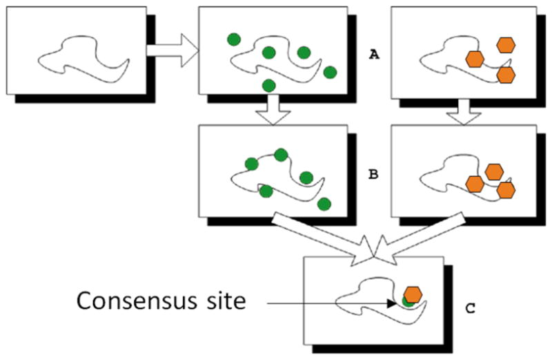
Schematic figure of computational solvent mapping using two probes. Each green circle and oranges hexagon represents a cluster for one of the two probe types. Figure 1c shows the consensus site where two probe clusters overlap, but occupy slightly different positions.

2. Software Requirements

This method requires a molecular viewer for preparation of crystal structures for mapping and analysis of results. This chapter assumes that PyMol (http://pymol.org), an Open Source molecular viewer available on Windows, Mac OS X, and Linux, will be used. Additionally, an Internet connection and web browser are required to use the various servers throughout the method.

3. Methods

3.1 Finding a Protein Structure

Computational solvent mapping techniques rely on the user to provide the 3-D structure of the protein. The vast majority of published structures of proteins can be found in the Protein Data Bank (PDB) in the PDB format. The simplest way to find a structure is by searching the PDB website (http://www.pdb.org) for the name of the protein. The PDB also provides an “Advanced Search”, where a sequence can be searched against the PDB using BLAST (Figure 2). The search by name relies on authors titling their structure, paper, or chains in the protein with the same name a user uses in their search. Thus, it can often be advantageous to use the sequence-based search.

Figure 2.

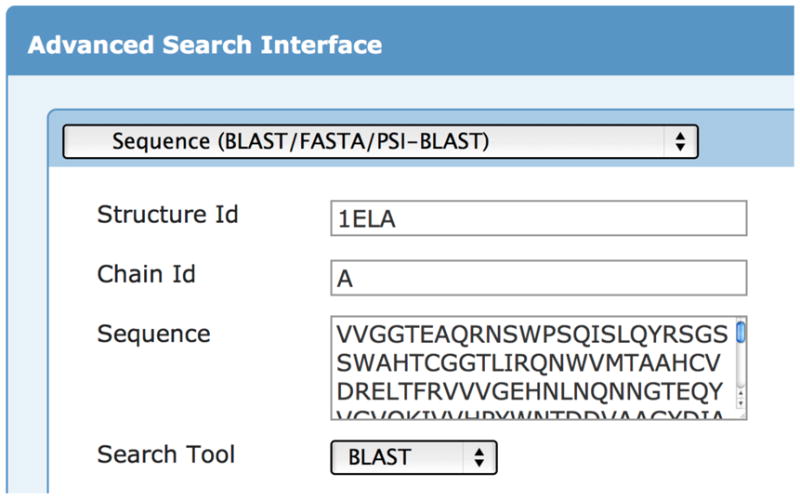
Advanced search interface for searching the Protein Data Bank (PDB) by sequence.

For many proteins, there will be more than one structure in the PDB. In general, the FTMap server produces better results from a high-resolution unbound crystal structure. Having ligands in the binding site often influences the shape of the site, sometimes disturbing the ability to detect hot spots. An initial search on the PDB website can be refined by whether the structure has ligands along with the experimental method (Figure 3). Additionally, the query results can be sorted by resolution. Note though that the PDB classifies many structures as having ligands even if they are unbound. If a structure has an innate metal ion, or if cryoprotectants such as glycerol are seen, the structure will be labeled as having a ligand, despite not having a ligand in the binding site of interest.

Figure 3.

Refining a query in the PDB by presence of ligands and experimental method.

3.2 Server Submission

The FTMap server is available for free use by academics at http://ftmap.bu.edu. After creating an account, you can submit jobs as shown in Figure 4. If you are using a structure from the pdb, you can specify the pdb id and the chains. Note that HETATM records within the pdb file are automatically stripped out. There are no parameters for the majority of HETATMs from the PDB on the server. The server does contain parameters for many common metals though, such as iron, magnesium, and zinc. If you want to include these, you should specify them as a chain by the letter ‘H’ for HETATM, followed by the residue name, followed by the chain id. In Figure 4, HZNA stands for the zinc from chain A of the protein. If using an NMR protein, the model can be specified (see Note 1).

Figure 4.

FTMap job submission interface.

If a protein has been prepared as a pdb file for mapping, as in preparing a single domain of a multi-domain protein (see Note 2), this file can be uploaded by clicking on Upload PDB in the interface. The chains can be specified as described above.

If you created a masking file (see Note 3), it may be uploaded under Advanced Options. Lastly, to look for binding sites in a protein-protein interaction site, a special PPI mode that has been incorporated into the FTMap server.

After submitting a protein through the server, you should wait for an e-mail informing you of job completion. Depending on the load on the server, a job can take from 2 hours to a full day.

3.3 Analysis of Results

After a job completes, three files will be available for download, a pdb file containing the mapping, and two text files with counts of nonbonded and hydrogen-bonded interactions to each residue on the protein (Figure 5).

Figure 5.

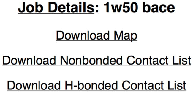
FTMap job download interface.

3.3.1 Analysis of Mapping

The pdb containing the mapping is specially formatted to be split into multiple objects when loaded into PyMol. Additionally, it is recommended to place the following code into a pymol startup file. This code should be placed file named pymolrc.py in your home directory on Windows (C:\Users\USERNAME\) or a file named .pymolrc in your home directory on Mac OS X (/Users/USERNAME/) or Linux (/home/USERNAME/). These functions allow you to easily color clusters by rank, disable and enable clusters, and rename the objects loaded in from an FTMap job. This last task is especially important if loading multiple FTMap jobs into a single PyMol Session as the object names may overwrite each other.

from pymol import cmd, util
def colorClusters():
      util.cbac('*.000.*')
      util.cbap('*.001.*')
      util.cbay('*.002.*')
      util.cbas('*.003.*')
      util.cbaw('*.004.*')
      util.cbab('*.005.*')
      util.cbao('*.006.*')
      util.cbag('*.007.*')
      util.cbam('*.008.*')
      util.cbak('*.009.*')
def disableClusters(rank='all'):
      if (rank == 'all'):
          cmd.disable('*.*.*')
      else:
          select = "*.%03d.*" % int(rank)
          cmd.disable(select)
def enableClusters(rank='all'):
      if (rank == 'all'):
          cmd.enable('*.*.*')
      else:
          select ="*.%03d.*" % int(rank)
          cmd.enable(select)
def renameFTMap(protname):
      stored.clusters=[]
      cmd.iterate('crosscluster* and index 1', 'stored.clusters.append(model)')
      for cluster in stored.clusters:
          namepieces = cluster.split('.')
          namepieces[0] = protname #set first element to protname
          if (namepieces[--−1] == "pdb"):
                namepieces.pop()
          name = '.'.join(namepieces)
          cmd.set_name(cluster, name)
      cmd.group(protname+'_clusters', protname+'.*')
      cmd.set_name('protein', protname)
cmd.extend('cc', colorClusters)
cmd.extend('colorClusters', colorClusters)
cmd.extend('dc', disableClusters)
cmd.extend('disableClusters', disableClusters)
cmd.extend('ec', enableClusters)
cmd.extend('enableClusters', enableClusters)
cmd.extend('rf', renameFTMap)
cmd.extend('renameFTMap', renameFTMap)

When the mapping is opened in PyMol, several objects are created. The protein submitted for mapping is labeled “protein”. The individual crossclusters from mapping are labeled “crosscluster.rank.population.pdb”. Each crosscluster represents a location where multiple different probe types clustered with a 4 Å radius. These locations are the hot spots for binding. In looking for a druggable pocket, there should be a large population crosscluster (population greater than 10) with several nearby crossclusters of lower population. An example in Figure 6a is the mapping of PDB 1w50, an apo structure of β-secretase. The largest crosscluster, with population 19, is seen in a pocket surrounded by a variety of other crossclusters. Drug-like molecules have been developed for β-secretase, such as the one shown in Figure 6b, a submicromolar inhibitor (18) that uses the hot spots defined by mapping.

Figure 6.

Figure 6a Mapping of apo β-secretase (1w50) showing a pocket that contains a large crosscluster with smaller cluster neighbors which (b) agree well with the binding of a submicromolar inhibitor (2ohu).

Figure 6b Mapping of apo β-secretase (1w50) showing a pocket that (a) contains a large crosscluster with smaller cluster neighbors which (b) agree well with the binding of a submicromolar inhibitor (2ohu).

If in analyzing the mapping, the majority of the results are going into an area between two structural domains rather than a well-defined pocket, the protein should be separated into the individual structural domains to be mapped independently (see Note 2). If the consensus site is in the location of a tightly bound coenzyme, but other druggable sites are desired, a masking file should be created to eliminate results in the region around the coenzyme (see Note 3).

3.3.2 Analysis of Contacts

While visual examination of the mapping provides a large amount of information that can be used for structural design of a molecule, analysis of the provided lists of hydrogen-bonded and nonbonded contacts made by probes in mapping can provide additional information on specific residues to target. These files have 4 columns, with the first three columns identifying the residue index, chain, and residue type. The fourth column contains the number of hydrogen-bond or nonbonded contacts the top 2000 results for each of the probes in mapping formed with a particular residue. The file can be sorted on this column using UNIX tools, as shown in Figure 7, on Mac OS X or Linux, or may be imported into a spreadsheet program such as Microsoft Excel to be sorted. In Figure 7, the results for the mapping of PDB 1w50, an apo β-secretase, are shown. The top two residues for hydrogen bonds are ASP 228 and ASP 32. These residues were found to form hydrogen bonds to a large number of fragments by Astex Therapeutics (19). The top two residues for nonbonded contacts are Phe108 and Leu30, which are used by the bulk of the submicromolar inhibitor shown in Figure 6b. The top hydrogen-bond and nonbonded contacts can provide information of use in structure-based drug design.

Figure 7.

Analysis of the top hydrogen-bonded and nonbonded contacts on Mac OS X or Linux.

Figure 8.

Derived data for PDB 1efv, showing that each method assigns two domains to chain A and a single domain to chain B.

Figure 9.

Mapping of domains to sequences from (a) SCOP, (b) CATH, (c) PFA

Figure 10.

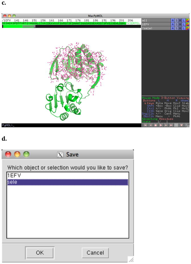
Preparation of a protein domain for mapping in PyMol by (a) loading of the PDB, (b) showing the sequence, (c) selection of the domain, and (d) saving of the selection object.

Figure 11.

Creation of a mask in the ATP binding region of a protein by (a) selection of the ATP analogue and (b) expansion of the selection into the site.

References

- 1.Clackson T, Wells JA. A hot spot of binding energy in a hormone-receptor interface. Science. 1995;267:383–386. doi: 10.1126/science.7529940. [DOI] [PubMed] [Google Scholar]
- 2.Mattos C, Ringe D. Locating and characterizing binding sites on proteins. Nat Biotechnol. 1996;14:595–599. doi: 10.1038/nbt0596-595. [DOI] [PubMed] [Google Scholar]
- 3.Hajduk PJ, Huth JR, Tse C. Predicting protein druggability. Drug Discov Today. 2005;10:1675–1682. doi: 10.1016/S1359-6446(05)03624-X. [DOI] [PubMed] [Google Scholar]
- 4.Hajduk PJ, Huth JR, Fesik SW. Druggability indices for proteintargets derived from NMR-based screening data. J Med Chem. 2005;48:2518–2525. doi: 10.1021/jm049131r. [DOI] [PubMed] [Google Scholar]
- 5.Allen KN, Bellamacina CR, Ding X, Jeffery CJ, Mattos C, Petsko GA, Ringe D. An experimental approach to mapping the binding surfaces of crystalline proteins. J Phys Chem. 1996;100:2605–2611. [Google Scholar]
- 6.English AC, Done SH, Caves LS, Groom CR, Hubbard RE. Locating interaction sites on proteins: the crystal structure of thermolysin soaked in 2% to 100% isopropanol. Proteins. 1999;37:6283640. [PubMed] [Google Scholar]
- 7.English AC, Groom CR, Hubbard RE. Experimental and computational mapping of the binding surface of a crystalline protein. Protein Eng. 2001;14:47359. doi: 10.1093/protein/14.1.47. [DOI] [PubMed] [Google Scholar]
- 8.Mattos C, Bellamacina CR, Peisach E, Pereira A, Vitkup D, Petsko GA, Ringe D. Multiple solvent crystal structures: probing binding sites, plasticity and hydration. J Mol Biol. 2006;357:1471–1482. doi: 10.1016/j.jmb.2006.01.039. [DOI] [PubMed] [Google Scholar]
- 9.Dennis S, Kortvelyesi T, Vajda S. Computational mapping identifies the binding sites of organic solvents on proteins. Proc Natl Acad Sci USA. 2002;99:4290–4295. doi: 10.1073/pnas.062398499. [DOI] [PMC free article] [PubMed] [Google Scholar]
- 10.Brenke R, Kozakov D, Chuang G-Y, Beglov D, Hall D, Landon MR, Mattos C, Vajda S. Fragment-based identification of druggable "hot spots" of proteins using Fourier domain correlation techniques. Bioinformatics. 2009;25:621–627. doi: 10.1093/bioinformatics/btp036. [DOI] [PMC free article] [PubMed] [Google Scholar]
- 11.Silberstein M, Dennis S, Brown L, III, Kortvelyesi T, Clodfelter K, Vajda S. Identification of substrate binding sites in enzymes by computational solvent mapping. J Molec Biol. 2003;332:1095–1113. doi: 10.1016/j.jmb.2003.08.019. [DOI] [PubMed] [Google Scholar]
- 12.Landon MR, Lancia DR, Jr, Yu J, Thiel SC, Vajda S. Identification of hot spots within druggable binding sites of proteins by computational solvent mapping. J Med Chem. 2007;50:1231–1240. doi: 10.1021/jm061134b. [DOI] [PubMed] [Google Scholar]
- 13.Vajda S, Guarnieri F. Characterization of protein-ligand interaction sites using experimental and computational methods. Current Opinion in Drug Design and Development. 2006;9:354–362. [PubMed] [Google Scholar]
- 14.Landon MR, Lieberman RL, Hoang QQ, Ju S, Caaveiro JM, Orwig SD, Kozakov D, Brenke R, Chuang G-Y, Beglov D, Vajda S, Petsko GA, Ringe D. Detection of ligand binding hot spots on protein surfaces via fragment-based methods: application to DJ-1 and glucocerebrosidase. J Comput Aided Mol Des. 2009;23:491–500. doi: 10.1007/s10822-009-9283-2. [DOI] [PMC free article] [PubMed] [Google Scholar]
- 15.Landon MR, Amaro RE, Baron R, Ngan C-H, Ozonoff D, McCammon JA, Vajda S. Novel druggable hot spots in avian influenza neuraminidase H5N1 revealed by computational solvent mapping of a reduced and representative receptor ensemble. Chem Biol Drug Des. 2008;71:106–116. doi: 10.1111/j.1747-0285.2007.00614.x. [DOI] [PMC free article] [PubMed] [Google Scholar]
- 16.Ngan C-H, Beglov D, Rudnitskay AN, Kozakov D, Waxman DJ, Vajda S. The structural basis of pregnane X receptor binding promiscuity. Biochemistry. 2009;48:11572–11581. doi: 10.1021/bi901578n. [DOI] [PMC free article] [PubMed] [Google Scholar]
- 17.Chuang G-Y, Kozakov D, Brenke R, Beglov D, Guarnieri F, Vajda S. Binding hot spots and amantadine orientation in the influenza a virus M2 proton channel. Biophys J. 2009;97(10):2846–2853. doi: 10.1016/j.bpj.2009.09.004. [DOI] [PMC free article] [PubMed] [Google Scholar]
- 18.Congreve M, Aharony D, Albert J, Callaghan O, Campbell J, Carr RA, Chessari G, Cowan S, Edwards PD, Frederickson M, McMenamin R, Murray CW, Patel S, Wallis N. Application of fragment screening by X-ray crystallography to the discovery of aminopyridines as inhibitors of beta-secretase. J Med Chem. 2007;50:1124–1132. doi: 10.1021/jm061197u. [DOI] [PubMed] [Google Scholar]
- 19.Murray CW, Callaghan O, Chessari G, Cleasby A, Congreve M, Frederickson M, Hartshorn MJ, McMenamin R, Patel S, Wallis N. Application of fragment screening by X-ray crystallography to beta-secretase. J Med Chem. 2007;50:1116–1123. doi: 10.1021/jm0611962. [DOI] [PubMed] [Google Scholar]